
Evaluation of Macrophyte Community Dynamics (2015–2020) in Southern Lake Garda (Italy) from Sentinel-2 Data

 ,
,  ,
,  ,
,  and
and
Abstract
:Featured Application
Abstract
1. Introduction
2. Materials and Method
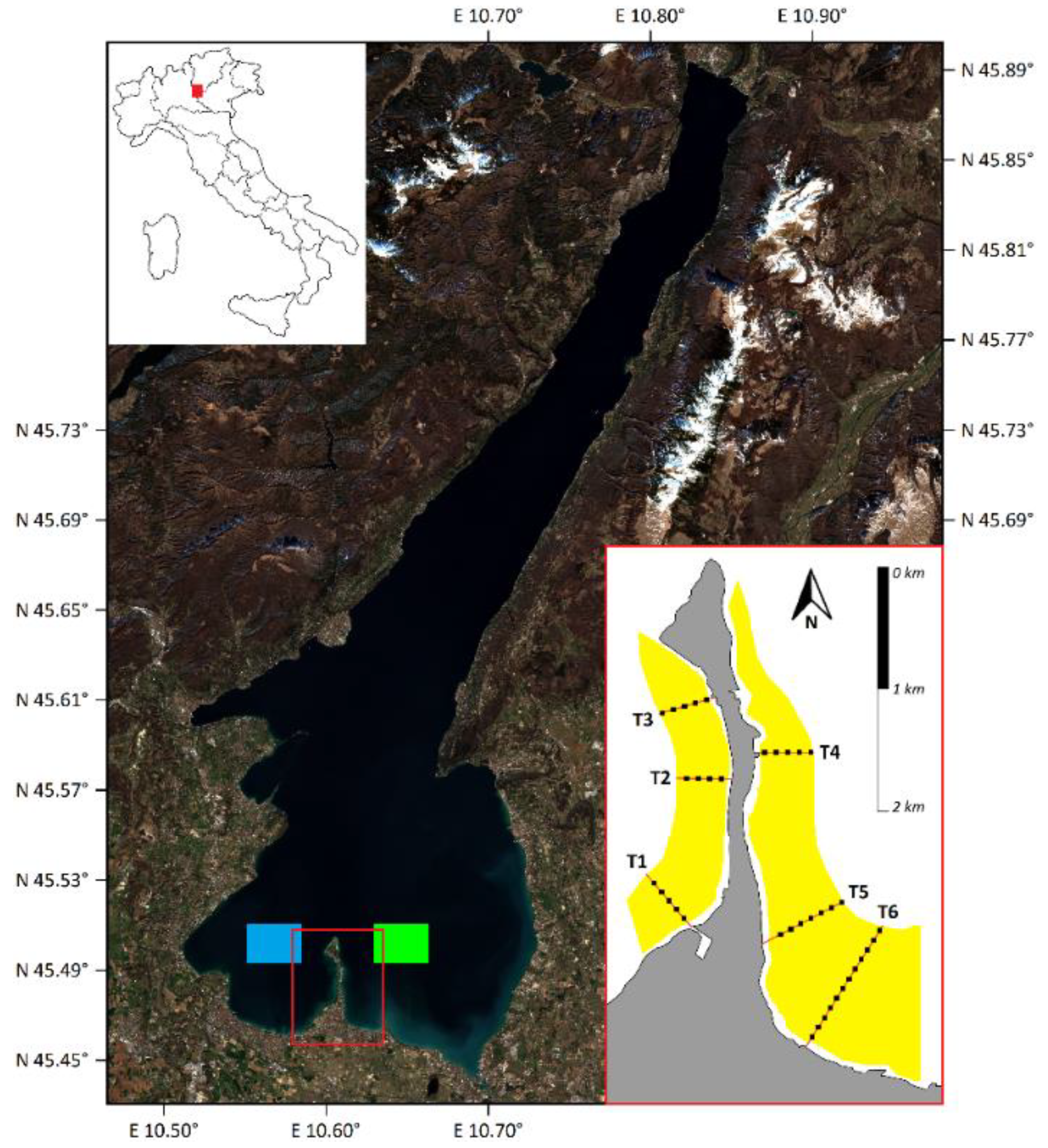
2.1. Study Area
2.2. Sentinel-2 Images Processing and Validation
2.3. Comparison between Sentinel-2 and Airborne Hyperspectral MIVIS
2.4. Ancillary Data
2.5. Statistical Analysis
3. Results
3.1. Evaluation of S2-Derived Products
3.2. Spatiotemporal Dynamics of Macrophyte Communities
3.3. Drivers of Macrophyte Density Patterns
4. Discussion
5. Conclusions
Supplementary Materials
Author Contributions
Funding
Institutional Review Board Statement
Informed Consent Statement
Data Availability Statement
Acknowledgments
Conflicts of Interest
References
- Jeppesen, E.; Brucet, S.; Naselli-Flores, L.; Papastergiadou, E.; Stefanidis, K.; Nõges, T.; Nõges, P.; Attayde, J.L.; Zohary, T.; Coppens, J.; et al. Ecological impacts of global warming and water abstraction on lakes and reservoirs due to changes in water level and related changes in salinity. Hydrobiologia 2015, 750, 201–227. [Google Scholar] [CrossRef]
- Woolway, R.I.; Sharma, S.; Weyhenmeyer, G.A.; Debolskiy, A.; Golub, M.; Mercado-Bettín, D.; Perroud, M.; Stepanenko, V.; Tan, Z.; Grant, L.; et al. Phenological shifts in lake stratification under climate change. Nat. Commun. 2021, 12, 2318. [Google Scholar] [CrossRef] [PubMed]
- Woolway, R.I.; Kraemer, B.M.; Lenters, J.D.; Merchant, C.J.; O’Reilly, C.M.; Sharma, S. Global lake responses to climate change. Nat. Rev. Earth Environ. 2020, 1, 388–403. [Google Scholar] [CrossRef]
- Ghirardi, N.; Bolpagni, R.; Bresciani, M.; Valerio, G.; Pilotti, M.; Giardino, C. Spatiotemporal dynamics of submerged aquatic vegetation in a deep lake from Sentinel-2 data. Water 2019, 11, 563. [Google Scholar] [CrossRef] [Green Version]
- Thomaz, S.M. Ecosystem services provided by freshwater macrophytes. Hydrobiologia. 2021, 1–21. [Google Scholar] [CrossRef]
- Bresciani, M.; Bolpagni, R.; Oggioni, A.; Giardino, C. Retrospective assessment of macrophytic communities in southern Lake Garda (Italy) from in situ and MIVIS. J. Limnol. 2012, 71, 180–190. [Google Scholar] [CrossRef] [Green Version]
- Bolpagni, R.; Laini, A.; Azzella, M.M. Short-term dynamics of submerged aquatic vegetation diversity and abundance in deep lakes. Appl. Veg. Sci. 2016, 19, 711–723. [Google Scholar] [CrossRef]
- Azzella, M.M.; Bresciani, M.; Nizzoli, D.; Bolpagni, R. Aquatic vegetation in deep lakes: Macrophyte co-occurrence patterns and environmental determinants. J. Limnol. 2017, 76, e19. [Google Scholar] [CrossRef] [Green Version]
- Yadav, S.; Yoneda, M.; Susaki, J.; Tamura, M.; Ishikawa, K.; Yamashiki, Y. A satellite-based assessment of the distribution and biomass of submerged aquatic vegetation in the optically shallow basin of Lake Biwa. Remote Sens. 2017, 9, 966. [Google Scholar] [CrossRef] [Green Version]
- Fritz, C.; Kuhwald, K.; Schneider, T.; Geist, J.; Oppelt, N. Sentinel-2 for mapping the spatio-temporal development of submerged aquatic vegetation at Lake Starnberg (Germany). J. Limnol. 2019, 78, 71–91. [Google Scholar] [CrossRef]
- Azzella, M.M.; Bolpagni, R.; Oggioni, A. A preliminary evaluation of lake morphometric traits influence on the maximum colonization depth of aquatic plants. J. Limnol. 2014, 73, 2. [Google Scholar] [CrossRef] [Green Version]
- Evtimova, V.V.; Donohue, I. Water-level fluctuations regulate the structure and functioning of natural lakes. Freshw. Biol. 2016, 61, 251–264. [Google Scholar] [CrossRef]
- Vejříková, I.; Vejřík, L.; Lepš, J.; Kočvara, L.; Sajdlová, Z.; Čtvrtlíková, M.; Peterka, J. Impact of herbivory and competition on lake ecosystem structure: Underwater experimental manipulation. Sci. Rep. 2018, 8, 12130. [Google Scholar] [CrossRef]
- Villa, P.; Bresciani, M.; Bolpagni, R.; Braga, F.; Bellingeri, D.; Giardino, C. Impact of upstream landslide on perialpine lake ecosystem: An assessment using multi-temporal satellite data. Sci. Total Environ. 2020, 720, 137627. [Google Scholar] [CrossRef]
- Jupp, B.J.; Spence, D.H.N. Limitations of Macrophytes in a Eutrophic Lake, Loch Leven: II. Wave Action, Sediments and Waterfowl Grazing. J. Ecol. 1977, 65, 431–446. [Google Scholar] [CrossRef]
- Schutten, J.; Dainty, J.; Davy, A.J. Root anchorage and its significance for submerged plants in shallow lakes. J. Ecol. 2005, 93, 556–571. [Google Scholar] [CrossRef]
- Zhao, F.; Fang, X.; Zhao, Z.; Chai, X. Effects of Water Level Fluctuations on the Growth Characteristics and Community Succession of Submerged Macrophytes: A Case Study of Yilong Lake, China. Water 2021, 13, 2900. [Google Scholar] [CrossRef]
- Zhao, D.; Jiang, H.; Cai, Y.; An, S. Artificial Regulation of Water Level and Its Effect on Aquatic Macrophyte Distribution in Taihu Lake. PLoS ONE 2012, 7, e44836. [Google Scholar] [CrossRef]
- Van Donk, E.; Otte, A. Effects of Grazing by Fish and Waterfowl on the Biomass and Species Composition of Submerged Macrophytes. Hydrobiologia 1996, 340, 285–290. [Google Scholar] [CrossRef]
- Sagerman, J.; Hansen, J.P.; Wikström, S.A. Effects of boat traffic and mooring infrastructure on aquatic vegetation: A systematic review and meta-analysis. Ambio 2020, 49, 517–530. [Google Scholar] [CrossRef] [Green Version]
- Dudgeon, D. Multiple threats imperil freshwater biodiversity in the Anthropocene. Curr. Biol. 2019, 29, R960–R967. [Google Scholar] [CrossRef] [PubMed]
- Directive, H. Council Directive 92/43/EEC of 21 May 1992 on the conservation of natural habitats and of wild fauna and flora. Off. J. Eur. Union 1992, 206, 7–50. [Google Scholar]
- Bolpagni, R.; Azzella, M.M.; Agostinelli, C.; Beghi, A.; Bettoni, E.; Brusa, G.; De Molli, C.; Formenti, R.; Galimberti, F.; Cerabolini, B.E. Integrating the water framework directive into the habitats directive: Analysis of distribution patterns of lacustrine EU habitats in lakes of Lombardy (northern Italy). J. Limnol. 2017, 76 (Suppl. S1), 75–83. [Google Scholar] [CrossRef]
- Directive 2000/60/EC of the European Parliament and of the Council of 23 October 2000 Establishing a Framework for Community Action in the Field of Water Policy. OJ L 327, 22.12.2000. 2000, pp. 1–51. Available online: https://ec.europa.eu/environment/water/water-framework/index_en.html/ (accessed on 13 December 2021).
- Jäger, P.; Pall, K.; Dumfarth, E. A method of mapping macrophytes in large lakes with regard to the requirements of the Water Framework Directive. Limnologica 2004, 34, 140–146. [Google Scholar] [CrossRef] [Green Version]
- Schaumburg, J.; Schranz, C.; Stelzer, D.; Hofmann, G. Action instructions for the ecological evaluation of lakes for implementation of the EU Water Framework Directive: Makrophytes and Phytobenthos. Bavar. Environ. Agency 2007, 69. Available online: https://www.planktonforum.eu/fileadmin/user_upload/instruction_protocol_lakes_2007.pdf/ (accessed on 4 November 2021).
- Oggioni, A.; Buzzi, F.; Bolpagni, R. Indici Macrofitici per la Valutazione della Qualità Ecologica dei Laghi: MacroIMMI e MTIspecies; Report 03.11; CNR-ISE: Pallanza, Italy, 2011; pp. 53–82. [Google Scholar]
- Fonseca, M.; Whitfield, P.E.; Kelly, N.M.; Bell, S.S. Modeling seagrass landscape pattern and associated ecological attributes. Ecol. Appl. 2002, 12, 218–237. [Google Scholar] [CrossRef]
- Fyfe, S.K. Spatial and temporal variation in spectral reflectance: Are seagrass species spectrally distinct? Limnol. Oceanogr. 2003, 48, 464–479. [Google Scholar] [CrossRef]
- Hestir, E.L.; Brando, V.E.; Bresciani, M.; Giardino, C.; Matta, E.; Villa, P.; Dekker, A.G. Measuring freshwater aquatic ecosystems: The need for a hyperspectral global mapping satellite mission. Remote Sens. Environ. 2015, 167, 181–195. [Google Scholar] [CrossRef] [Green Version]
- Silva, T.S.; Costa, M.P.; Melack, J.M.; Novo, E.M. Remote sensing of aquatic vegetation: Theory and applications. Environ. Monit. Assess. 2008, 140, 131–145. [Google Scholar] [CrossRef]
- Milan, M.; Bigler, C.; Salmaso, N.; Guella, G.; Tolotti, M. Multiproxy reconstruction of a large and deep subalpine lake’s ecological history since the Middle Ages. J. Great Lakes Res. 2015, 41, 982–994. [Google Scholar] [CrossRef]
- Giardino, C.; Bartoli, M.; Candiani, G.; Bresciani, M.; Pellegrini, L. Recent changes in macrophyte colonisation patterns: An imaging spectrometry-based evaluation of southern Lake Garda (northern Italy). J. Appl. Remote Sens. 2007, 1, 011509. [Google Scholar] [CrossRef]
- Zhang, Y.; Jeppesen, E.; Liu, X.; Qin, B.; Shi, K.; Zhou, Y.; Thomaz, S.M.; Deng, J. Global loss of aquatic vegetation in lakes. Earth Sci. Rev. 2017, 173, 259–265. [Google Scholar] [CrossRef]
- Sayer, C.D.; Burgess, A.M.Y.; Kari, K.; Davidson, T.A.; Peglar, S.; Yang, H.; Rose, N. Long-term dynamics of submerged macrophytes and algae in a small and shallow, eutrophic lake: Implications for the stability of macrophyte-dominance. Freshw. Biol. 2010, 55, 565–583. [Google Scholar] [CrossRef]
- Phillips, G.; Willby, N.; Moss, B. Submerged macrophyte decline in shallow lakes: What have we learnt in the last forty years? Aquat. Bot. 2016, 135, 37–45. [Google Scholar] [CrossRef] [Green Version]
- Cristofor, S.; Vadineanu, A.; Sarbu, A.; Postolache, C.; Dobre, R.; Adamescu, M. Long-term changes of submerged macrophytes in the Lower Danube Wetland System. Hydrobiologia 2003, 506, 625–634. [Google Scholar] [CrossRef]
- Sayer, C.D.; Davidson, T.A.; Jones, J.I. Seasonal dynamics of macrophytes and phytoplankton in shallow lakes: A eutrophication-driven pathway from plants to plankton? Freshw. Biol. 2010, 55, 500–513. [Google Scholar] [CrossRef]
- Azzella, M.M.; Rosati, L.; Iberite, M.; Bolpagni, R.; Blasi, C. Changes in aquatic plants in the Italian volcanic-lake system detected using current data and historical records. Aquat. Bot. 2014, 112, 41–47. [Google Scholar] [CrossRef]
- Bai, G.; Zhang, Y.; Yan, P.; Yan, W.; Kong, L.; Wang, L.; Wang, C.; Liu, Z.; Liu, B.; Ma, J.; et al. Spatial and seasonal variation of water parameters, sediment properties, and submerged macrophytes after ecological restoration in a long-term (6 year) study in Hangzhou west lake in China: Submerged macrophyte distribution influenced by environmental variables. Water Res. 2020, 186, 116379. [Google Scholar] [CrossRef]
- Murphy, F.; Schmieder, K.; Baastrup-Spohr, L.; Pedersen, O.; Sand-Jensen, K. Five decades of dramatic changes in submerged vegetation in Lake Constance. Aquat. Bot. 2018, 144, 31–37. [Google Scholar] [CrossRef] [Green Version]
- Salmaso, N.; Mosello, R. Limnological research in the deep southern subalpine lakes: Synthesis, directions and perspectives. Adv. Oceanogr. Limnol. 2010, 1, 29–66. [Google Scholar] [CrossRef]
- Salmaso, N.; Mosello, R.; Garibaldi, L.; Decet, F.; Brizzio, M.C.; Cordella, P. Vertical mixing as a determinant of trophic status in deep lakes: A case study from two lakes south of the Alps (Lake Garda and Lake Iseo). J. Limnol. 2003, 62, 33–41. [Google Scholar] [CrossRef]
- Hinegk, L.; Adami, L.; Zolezzi, G.; Tubino, M. Implications of water resources management on the long-term regime of Lake Garda (Italy). J. Environ. Manag. 2022, 301, 113893. [Google Scholar] [CrossRef] [PubMed]
- Sauro, U. La macchina idraulica. In Il Lago di Garda. Cierre Edizioni; Sauro, U., Simoni, C., Turri, E., Varanini, G.M., Eds.; Cierre Edizioni: Caselle, Italy, 2001; p. 496. [Google Scholar]
- Minella, M.; Leoni, B.; Salmaso, N.; Savoye, L.; Sommaruga, R.; Vione, D. Long-term trends of chemical and modelled photochemical parameters in four Alpine lakes. Sci. Total Environ. 2016, 541, 247–256. [Google Scholar] [CrossRef] [PubMed]
- Salmaso, N.; Boscaini, A.; Capelli, C.; Cerasino, L. Ongoing ecological shifts in a large lake are driven by climate change and eutrophication: Evidences from a three-decade study in Lake Garda. Hydrobiologia 2018, 824, 177–195. [Google Scholar] [CrossRef]
- Salmaso, N. Long-term phytoplankton community changes in a deep subalpine lake: Responses to nutrient availability and climatic fluctuations. Freshw. Biol. 2010, 55, 825–846. [Google Scholar] [CrossRef]
- Premazzi, G.; Dalmiglio, A.; Cardoso, A.C.; Chiaudani, G. Lake management in Italy: The implications of the Water Framework Directive. Lakes Reserv. Res. Manag. 2003, 8, 41–59. [Google Scholar] [CrossRef]
- Bolpagni, R.; Bettoni, E.; Bonomi, F.; Bresciani, M.; Caraffini, K.; Costaraoss, S.; Giacomazzi, F.; Monauni, C.; Montanari, P.; Mosconi, M.C.; et al. Charophytes of the lake Garda (Northern Italy): A preliminary assessment of diversity and distribution. J. limnol. 2013, 72, e31. [Google Scholar] [CrossRef] [Green Version]
- Copernicus Open Access Hub. Available online: https://scihub.copernicus.eu/ (accessed on 1 November 2021).
- ONDA Catalogue. Available online: https://catalogue.onda-dias.eu/catalogue/ (accessed on 1 November 2021).
- Vermote, E.F.T.D.; Tanré, D.; Deuzé, J.L.; Herman, M.; Morcrette, J.J.; Kotchenova, S.Y. Second simulation of a satellite signal in the solar spectrum-vector (6SV). 6S User Guide Vers. 2006, 3, 1–55. [Google Scholar]
- Bresciani, M.; Cazzaniga, I.; Austoni, M.; Sforzi, T.; Buzzi, F.; Morabito, G.; Giardino, C. Mapping phytoplankton blooms in deep subalpine lakes from Sentinel-2A and Landsat-8. Hydrobiologia 2018, 824, 197–214. [Google Scholar] [CrossRef] [Green Version]
- Cazzaniga, I.; Bresciani, M.; Colombo, R.; Della Bella, V.; Padula, R.; Giardino, C. A comparison of Sentinel-3-OLCI and Sentinel-2-MSI-derived Chlorophyll-a maps for two large Italian lakes. Remote Sens. Lett. 2019, 10, 978–987. [Google Scholar] [CrossRef]
- AERONET Aerosol Robotic Network. Available online: https://aeronet.gsfc.nasa.gov/ (accessed on 18 November 2021).
- GIOVANNI the Bridge between Data and Science. Available online: https://giovanni.gsfc.nasa.gov/giovanni/ (accessed on 18 November 2021).
- Giardino, C.; Candiani, G.; Bresciani, M.; Lee, Z.; Gagliano, S.; Pepe, M. BOMBER: A tool for estimating water quality and bottom properties from remote sensing images. Comput. Geosci. 2012, 45, 313–318. [Google Scholar] [CrossRef]
- Giardino, C.; Bresciani, M.; Cazzaniga, I.; Schenk, K.; Rieger, P.; Braga, F.; Matta, E.; Brando, V.E. Evaluation of multi-resolution satellite sensors for assessing water quality and bottom depth of Lake Garda. Sensors 2014, 14, 24116–24131. [Google Scholar] [CrossRef] [PubMed] [Green Version]
- Bresciani, M.; Giardino, C.; Lauceri, R.; Matta, E.; Cazzaniga, I.; Pinardi, M.; Lami, A.; Austoni, M.; Viaggiu, E.; Congestri, R.; et al. Earth observation for monitoring and mapping of cyanobacteria blooms. Case studies on five Italian lakes. J. Limnol. 2017, 76, 127–139. [Google Scholar] [CrossRef] [Green Version]
- Free, G.; Bresciani, M.; Pinardi, M.; Ghirardi, N.; Luciani, G.; Caroni, R.; Giardino, C. Detecting Climate Driven Changes in Chlorophyll-a in Deep Subalpine Lakes Using Long Term Satellite Data. Water 2021, 13, 866. [Google Scholar] [CrossRef]
- Roelfsema, C.; Kovacs, E.; Ortiz, J.C.; Wolff, N.H.; Callaghan, D.; Wettle, M.; Ronan, M.; Hamylton, S.M.; Mumby, P.J.; Phinn, S. Coral reef habitat mapping: A combination of object-based image analysis and ecological modelling. Remote Sens. Environ. 2018, 208, 27–41. [Google Scholar] [CrossRef]
- Di Donato, V.; Reynolds, E.; Picheta, R. All of Italy Is in Lockdown as Coronavirus Cases Rise. 2020. Available online: https://edition.cnn.com/2020/03/09/europe/coronavirus-italy-lockdown-intl/ (accessed on 4 May 2021).
- Harlan, C.; Pitrelli, S. Italy’s Coronavirus Lockdown Upends the Most Basic Routines and Joys. 2020. Available online: https://www.washingtonpost.com/world/italy-coronavirus-lockdown/2020/03/10/ (accessed on 4 May 2021).
- Lazzerini, M.; Putoto, G. COVID-19 in Italy: Momentous decisions and many uncertainties. Lancet Glob. Health 2020, 8, e641–e642. [Google Scholar] [CrossRef] [Green Version]
- Vis, C.; Hudon, C.; Carignan, R. An evaluation of approaches used to determine the distribution and biomass of emergent and submerged aquatic macrophytes aver large spatial scales. Aquat. Bot. 2003, 77, 187–201. [Google Scholar] [CrossRef]
- Bolpagni, R.; Pierobon, E.; Longhi, D.; Nizzoli, D.; Bartoli, M.; Tomaselli, M.; Viaroli, P. Diurnal exchanges of CO2 and CH4 across the water-atmosphere interface in a water chestnut meadow (Trapa natans L.). Aquat. Bot. 2007, 87, 43–48. [Google Scholar] [CrossRef]
- Pierobon, E.; Bolpagni, R.; Bartoli, M.; Viaroli, P. Net primary production and seasonal CO2 and CH4 fluxes in a Trapa natans L. meadow. J. Limnol. 2010, 69, 225–234. [Google Scholar] [CrossRef] [Green Version]
- ARPA Veneto. Available online: https://www.arpa.veneto.it/temi-ambientali/acqua/acque-interne/acque-superficiali/laghi/dati (accessed on 2 December 2021).
- Crétaux, J.F.; Merchant, C.J.; Duguay, C.; Simis, S.; Calmettes, B.; Bergé-Nguyen, M.; Wu, Y.; Zhang, D.; Carrea, L.; Liu, X.; et al. ESA Lakes Climate Change Initiative (Lakes_cci): Lake Products; Version 1.0; Centre for Environmental Data Analysis: Didcot, UK, 2020. [Google Scholar] [CrossRef]
- Longoni, V.; Fasola, M. Censimento Annuale degli Uccelli Acquatici Svernanti in Lombardia. Resoconto 2015; Regione Lombardia: Milano, Italy, 2015. [Google Scholar]
- Longoni, V.; Fasola, M. Censimento Annuale degli Uccelli Acquatici Svernanti in Lombardia. Resoconto 2016; Regione Lombardia: Milano, Italy, 2016. [Google Scholar]
- Longoni, V.; Fasola, M. Censimento Annuale degli Uccelli Acquatici Svernanti in Lombardia. Resoconto 2017; Regione Lombardia: Milano, Italy, 2017. [Google Scholar]
- Longoni, V.; Fasola, M. Le Popolazioni di Uccelli Acquatici Svernanti in Lombardia, 2018; Regione Lombardia: Milano, Italy, 2018. [Google Scholar]
- Longoni, V.; Fasola, M. Le Popolazioni di Uccelli Acquatici Svernanti in Lombardia, 2019; Regione Lombardia: Milano, Italy, 2019. [Google Scholar]
- Longoni, V.; Fasola, M. Le Popolazioni di Uccelli Acquatici Svernanti in Lombardia, 2020; Regione Lombardia: Milano, Italy, 2020. [Google Scholar]
- Özgencil, İ.K.; Beklioğlu, M.; Özkan, K.; Tavşanoğlu, Ç.; Fattorini, N. Changes in Functional Composition and Diversity of Waterbirds: The Roles of Water Level and Submerged Macrophytes. Freshw. Biol. 2020, 65, 1845–1857. [Google Scholar] [CrossRef]
- AIPO Agenzia Interregionale Per Il Fiume Po. Available online: https://www.agenziapo.it/content/monitoraggio-idrografico-0 (accessed on 29 October 2021).
- Provincia di Brescia. Available online: http://turismoweb.provincia.brescia.it/statistiche/index.php (accessed on 23 November 2021).
- COPERNICUS Climate Data Store. Available online: https://cds.climate.copernicus.eu/cdsapp#!/home (accessed on 2 December 2021).
- Carter, D.J.T. Prediction of Wave Height and Period for a Constant Wind Velocity Using the JONSWAP Results. Ocean Eng. 1982, 9, 17–33. [Google Scholar] [CrossRef]
- ECMWF: ERA5 Data and Documentation. Available online: https://confluence.ecmwf.int/display/CKB/ERA5%3A+data+documentation (accessed on 17 November 2021).
- McCune, B. Nonparametric Multiplicative Regression for Habitat Modeling; Oregon State University: Corvallis, OR, USA, 2006. [Google Scholar]
- Carslaw, D.C.; Ropkins, K. Openair—An R Package for Air Quality Data Analysis. Environ. Modell. Softw. 2012, 27, 52–61. [Google Scholar] [CrossRef]
- R Core Team, R. A Language and Environment for Statistical Computing; R Foundation for Statistical Computing: Vienna, Austria, 2019. [Google Scholar]
- McCune, B.; Mefford, M.J. HyperNiche. Nonparametric Multiplicative Habitat Modeling; Version 2.25; MjM Software: Corvallis, OR, USA, 2009. [Google Scholar]
- Fritz, C.; Dörnhöfer, K.; Schneider, T.; Geist, J.; Oppelt, N. Mapping submerged aquatic vegetation using RapidEye satellite data: The example of Lake Kummerow (Germany). Water 2017, 9, 510. [Google Scholar] [CrossRef] [Green Version]
- Amadori, M.; Zamparelli, V.; De Carolis, G.; Fornaro, G.; Toffolon, M.; Bresciani, M.; Giardino, C.; De Santi, F. Monitoring Lakes Surface Water Velocity with SAR: A Feasibility Study on Lake Garda, Italy. Remote Sens. 2021, 13, 2293. [Google Scholar] [CrossRef]
- Randall, R.G.; Minns, C.K.; Cairns, V.W.; Moore, J.E. The Relationship between an Index of Fish Production and Submerged Macrophytes and Other Habitat Features at Three Littoral Areas in the Great Lakes. Can. J. Fish. Aquat. Sci. 1996, 53, 35–44. [Google Scholar] [CrossRef]
- Weatherhead, M.A.; James, M.R. Distribution of Macroinvertebrates in Relation to Physical and Biological Variables in the Littoral Zone of Nine New Zealand Lakes. Hydrobiologia 2001, 462, 115–129. [Google Scholar] [CrossRef]
- Free, G.; Bowman, J.; McGarrigle, M.; Caroni, R.; Donnelly, K.; Tierney, D.; Trodd, W.; Little, R. The Identification, Characterization and Conservation Value of Isoetid Lakes in Ireland. Aquat. Conserv. Mar. Freshw. Ecosyst. 2008, 19, 264–273. [Google Scholar] [CrossRef]
- Lodge, D.M. Herbivory on Freshwater Macrophytes. Aquat. Bot. 1991, 41, 195–224. [Google Scholar] [CrossRef]
- Ciutti, F.; Beltrami, M.E.; Confortini, I.; Cianfanelli, S.; Cappelletti, C. Non-Indigenous Invertebrates, Fish and Macrophytes in Lake Garda (Italy). J. Limnol. 2011, 70, 315–320. [Google Scholar] [CrossRef] [Green Version]
- Blindow, I. Decline of Charophytes during Eutrophication: Comparison with Angiosperms. Freshw. Biol. 1992, 28, 9–14. [Google Scholar] [CrossRef]
- Søndergaard, M.; Jensen, J.P.; Jeppesen, E. Role of Sediment and Internal Loading of Phosphorus in Shallow Lakes. Hydrobiologia 2003, 506, 135–145. [Google Scholar] [CrossRef]
- Phillips, G.L.; Eminson, D.; Moss, B. A Mechanism to Account for Macrophyte Decline in Progressively Eutrophicated Freshwaters. Aquat. Bot. 1978, 4, 103–126. [Google Scholar] [CrossRef]
- Free, G.; Bowman, J.; Caroni, R.; Donnelly, K.; Little, R.; McGarrigle, M.L.; Tierney, D.; Kennedy, N.; Allott, N.; Irvine, K. The Identification of Lake Types Using Macrophyte Community Composition in Ireland. Verh. Des. Int. Ver. Limnol. 2005, 29, 296–299. [Google Scholar] [CrossRef]
- Rogora, M.; Buzzi, F.; Dresti, C.; Leoni, B.; Lepori, F.; Mosello, R.; Patelli, M.; Salmaso, N. Climatic Effects on Vertical Mixing and Deep-Water Oxygen Content in the Subalpine Lakes in Italy. Hydrobiologia 2018, 824, 33–50. [Google Scholar] [CrossRef]
- Rädler, A.T.; Groenemeijer, P.H.; Faust, E.; Sausen, R.; Púčik, T. Frequency of Severe Thunderstorms across Europe Expected to Increase in the 21st Century Due to Rising Instability. Clim. Atmos. Sci. 2019, 2, 1–5. [Google Scholar] [CrossRef]
- Ranasinghe, R.; Ruane, A.C.; Vautard, R.; Arnell, N.; Coppola, E.; Cruz, F.A.; Dessai, S.; Islam, A.S.; Rahimi, M.; Ruiz Carrascal, D.; et al. Chapter 12: Climate Change Information for Regional Impact and for Risk Assessment. In Climate Change 2021: The Physical Science Basis; Contribution of Working Group I to the Sixth Assessment Report of the Intergovernmental Panel on Climate Change; Cambridge University Press: Cambridge, UK, 2021. [Google Scholar]
- Braga, F.; Scarpa, G.M.; Brando, V.E.; Manfè, G.; Zaggia, L. COVID-19 lockdown measures reveal human impact on water transparency in the Venice Lagoon. Sci. Total Environ. 2020, 736, 139612. [Google Scholar] [CrossRef]
- Temmink, R.J.M.; Dorenbosch, M.; Lamers, L.P.M.; Smolders, A.J.P.; Rip, W.; Lengkeek, W.; Didderen, K.; Fivash, G.S.; Bouma, T.J.; van der Heide, T. Growth forms and life-history strategies predict the occurrence of aquatic macrophytes in relation to environmental factors in a shallow peat lake complex. Hydrobiologia 2021, 848, 3987–3999. [Google Scholar] [CrossRef]


| Seasons | Date | |||||
|---|---|---|---|---|---|---|
| Spring | NA | 23/03/2016 | 28/03/2017 | 23/03/2018 | 23/03/2019 | 24/03/2020 |
| NA | 19/04/2016 | 17/05/2017 | 22/04/2018 | 17/04/2019 | 23/04/2020 | |
| Summer | 04/07/2015 | 28/06/2016 | 03/07/2017 | 18/06/2018 | 13/06/2019 | 02/06/2020 |
| 03/08/2015 | 17/08/2016 | 02/08/2017 | 23/07/2018 | 23/07/2019 | 27/07/2020 | |
| Autumn | 12/09/2015 | 19/09/2016 | 21/09/2017 | 19/09/2018 | 14/09/2019 | 30/09/2020 |
| 25/09/2015 | 16/10/2016 | 16/10/2017 | 04/10/2018 | 11/10/2019 | 08/10/2020 | |
| Year—(Season) | Area (km2) | Percentage (%) | ||||
|---|---|---|---|---|---|---|
| BS | SRM | DRM | BS | SRM | DRM | |
| 2015—Spring | NA | NA | NA | NA | NA | NA |
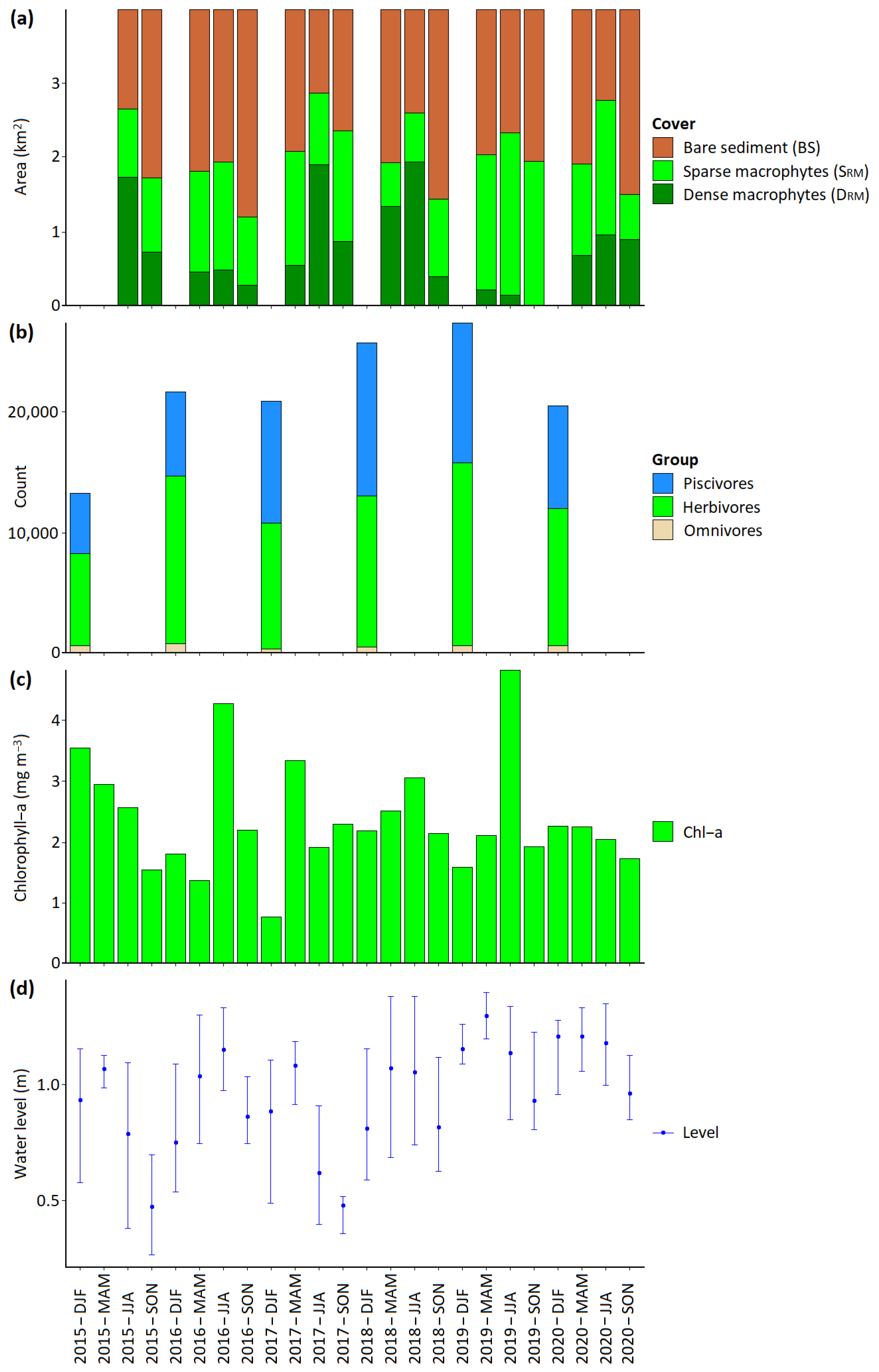
| 2015—Summer | 1.335 | 0.919 | 1.717 | 33.62 | 23.14 | 43.24 |
| 2015—Autumn | 2.263 | 0.994 | 0.714 | 56.99 | 25.03 | 17.98 |
| 2016—Spring | 2.173 | 1.356 | 0.442 | 54.72 | 34.15 | 11.13 |
| 2016—Summer | 2.056 | 1.446 | 0.469 | 51.78 | 36.41 | 11.81 |
| 2016—Autumn | 2.783 | 0.921 | 0.267 | 70.08 | 23.19 | 6.72 |
| 2017—Spring | 1.912 | 1.525 | 0.534 | 48.15 | 38.40 | 13.45 |
| 2017—Summer | 1.128 | 0.962 | 1.881 | 28.41 | 24.23 | 47.37 |
| 2017—Autumn | 1.633 | 1.483 | 0.855 | 41.12 | 37.35 | 21.53 |
| 2018—Spring | 2.061 | 0.583 | 1.327 | 51.90 | 14.68 | 33.42 |
| 2018—Summer | 1.390 | 0.664 | 1.917 | 35.00 | 16.72 | 48.27 |
| 2018—Autumn | 2.545 | 1.039 | 0.387 | 64.09 | 26.16 | 9.75 |
| 2019—Spring | 1.947 | 1.819 | 0.205 | 49.03 | 45.81 | 5.16 |
| 2019—Summer | 1.653 | 2.196 | 0.122 | 41.63 | 55.30 | 3.07 |
| 2019—Autumn | 2.035 | 1.935 | 0.001 | 52.25 | 48.73 | 0.03 |
| 2020—Spring | 2.071 | 1.242 | 0.658 | 52.15 | 31.28 | 16.57 |
| 2020—Summer | 1.221 | 1.808 | 0.942 | 30.75 | 45.53 | 23.72 |
| 2020—Autumn | 2.483 | 0.616 | 0.872 | 62.53 | 15.51 | 21.96 |
| Year—(Day) | Area (km2) | Δ Area (km2) | ||||
|---|---|---|---|---|---|---|
| SRM | DRM | RM | Δ SRM | Δ DRM | Δ RM | |
| 23/03/2016 | 0.925 | 1.505 | 2.430 | −0.641 | −1.107 | −1.748 |
| 19/04/2016 | 0.284 | 0.398 | 0.682 | |||
| 28/03/2017 | 0.688 | 1.578 | 2.266 | +0.380 | −1.491 | −1.111 |
| 17/05/2017 | 1.068 | 0.087 | 1.155 | |||
| 23/03/2018 | 0.447 | 1.578 | 2.025 | +0.253 | −0.613 | −0.360 |
| 22/04/2018 | 0.700 | 0.956 | 1.665 | |||
| 23/03/2019 | 2.293 | 0.279 | 2.572 | −1.225 | +0.282 | −0.943 |
| 17/04/2019 | 1.068 | 0.561 | 1.629 | |||
| 24/03/2020 | 1.068 | 0.784 | 1.852 | +0.011 | +0.044 | +0.055 |
| 23/04/2020 | 1.079 | 0.828 | 1.907 | |||
| Response Var. | xR2 | Ave. Size | Var.1 | Tol. | Sen. | Var.2 | Tol. | Sen | Var.3 | Tol. | Sen. | p |
|---|---|---|---|---|---|---|---|---|---|---|---|---|
| RM | 0.39 | 1.92 | time | 12.8 | 0.02 | season | 0.0 | NA | Secchi | 1.2 | 0.18 | 0.01 |
| RM | 0.44 | 2.35 | time | 12.8 | 0.03 | season | 0.0 | NA | Level_mean | 0.2 | 0.15 | 0.03 |
| RM | 0.40 | 2.64 | time | 12.8 | 0.02 | season | 0.0 | NA | Sum Herb | 3368 | 0.09 | 0.02 |
| RM | 0.39 | 3.17 | time | 12.8 | 0.01 | season | 0.0 | NA | DJF_Wave H | 0.0 | 0.05 | 0.03 |
| RM | 0.51 | 2.50 | time | 12.8 | 0.01 | season | 0.0 | NA | Chl–a | 0.9 | 0.13 | 0.01 |
| DRM | 0.32 | 2.21 | time | 12.8 | 0.02 | season | 0.0 | NA | Chl–a | 0.7 | 0.23 | 0.06 |
| Year | Potential Drivers | Response | Implication for Following Year | Herbivore/Macrophyte Change |
|---|---|---|---|---|
| 2015 | Herbivore bird population 7589. Winter wind mostly calm. Summer Chl–a was 2.6 mg m−3. Spring lake level was 1.06 m. | Macrophyte cover normal. | Lower herbivore bird grazing earlier in the year may have allowed an increase in macrophyte growth in subsequent months and lead to more foraging the following year. | |
| 2016 | Herbivore population increases to 13,908. High winter wind speed recorded (red in Figure S3). Summer Chl–a increases to 4.3 mg m−3. Spring lake level was 1.03 m. | Lowest total macrophyte cover in timeseries for MAM, JJA, SON recorded. | Lower macrophyte cover and lower density in SON will mean less foraging for birds. | ↑↓ |
| 2017 | Herbivore population declines to 10,327. Winter wind mostly calm. Summer Chl–a was 1.9 mg m−3. Spring lake level was 1.08 m. | An increase in Piscivores recorded, Macrophytes show recovery in subsequent months. | Recovery of macrophytes will mean more foraging for birds. | ↓↑ |
| 2018 | Herbivore population increases to 12,512. Winter wind mostly calm. Summer Chl–a was 3.0 mg m−3. Spring lake level was 1.07 m. | Macrophytes remain at similar or slightly lower levels. | Normal. | ↑→ |
| 2019 | Herbivore population continues recovery and reaches highest level of 15,074. Winter wind mostly calm but storm in May. Spring had higher water levels (1.29 m). Summer Chl–a increases to highest for the timeseries of 4.8 mg m−3. | Area of dense macrophytes is reduced to minimum of the timeseries. Total macrophytes in summer lower than previous two years. | Reduction in density of macrophytes may have implications for foraging. | ↑↓ |
| 2020 | Herbivore population declines to 11,326. Winter wind mostly calm. 55.7% reduction in tourist numbers likely to reduce erosion/turbidity from boat wakes. Summer Chl–a was 2.0 mg m−3. Spring lake level was 1.2 m. | Area of dense macrophytes recovers. Total macrophytes in summer return to higher levels. Piscivores decline. | NA | ↓↑ |
Publisher’s Note: MDPI stays neutral with regard to jurisdictional claims in published maps and institutional affiliations. |
© 2022 by the authors. Licensee MDPI, Basel, Switzerland. This article is an open access article distributed under the terms and conditions of the Creative Commons Attribution (CC BY) license (https://creativecommons.org/licenses/by/4.0/).
Share and Cite
Ghirardi, N.; Bresciani, M.; Free, G.; Pinardi, M.; Bolpagni, R.; Giardino, C. Evaluation of Macrophyte Community Dynamics (2015–2020) in Southern Lake Garda (Italy) from Sentinel-2 Data. Appl. Sci. 2022, 12, 2693. https://doi.org/10.3390/app12052693
Ghirardi N, Bresciani M, Free G, Pinardi M, Bolpagni R, Giardino C. Evaluation of Macrophyte Community Dynamics (2015–2020) in Southern Lake Garda (Italy) from Sentinel-2 Data. Applied Sciences. 2022; 12(5):2693. https://doi.org/10.3390/app12052693
Chicago/Turabian StyleGhirardi, Nicola, Mariano Bresciani, Gary Free, Monica Pinardi, Rossano Bolpagni, and Claudia Giardino. 2022. "Evaluation of Macrophyte Community Dynamics (2015–2020) in Southern Lake Garda (Italy) from Sentinel-2 Data" Applied Sciences 12, no. 5: 2693. https://doi.org/10.3390/app12052693
APA StyleGhirardi, N., Bresciani, M., Free, G., Pinardi, M., Bolpagni, R., & Giardino, C. (2022). Evaluation of Macrophyte Community Dynamics (2015–2020) in Southern Lake Garda (Italy) from Sentinel-2 Data. Applied Sciences, 12(5), 2693. https://doi.org/10.3390/app12052693