Article

Fingerprinting Organochlorine Groundwater Plumes Based on Non-Invasive ERT Technology at a Chemical Plant

1
Key Laboratory of Groundwater Resources and Environment, Jilin University, Ministry of Education, Changchun 130021, China
2
Jilin Provincial Key Laboratory of Water Resources and Environment, Jilin University, Changchun 130021, China
3
Key Lab of Eco-Restoration of Regional Contaminated Environment, Shenyang University, Ministry of Education, Shenyang 110044, China
*
Author to whom correspondence should be addressed.
Appl. Sci. 2022, 12(6), 2816; https://doi.org/10.3390/app12062816
Submission received: 7 February 2022 / Revised: 27 February 2022 / Accepted: 4 March 2022 / Published: 9 March 2022

Abstract

:
The refined characterization of groundwater pollution is an important prerequisite for efficient and effective remediation. A high-resolution survey of a contaminated site in a chemical pesticide factory was carried out using non-invasive geophysical sensing technology. Modern electrical resistivity tomography (ERT) technology can rapidly identify and characterize the groundwater pollution plumes of organochlorine pesticides, which was demonstrated in this study by the significantly abnormal resistivity sensing in stratums and aquifers under the raw material tanks, production, and loading areas. The results were found to be highly consistent with the ERT sensing results achieved via incorporating borehole sampling and hydrochemical analysis. With high abnormal resistivity, the range of contamination within the profile was characterized on the meter level. We also unexpectedly found new pollution and explained its source. This study confirmed that the modern refined ERT method has a high feasibility and accuracy in characterizing the spatial distribution of organochlorine pesticide plumes in groundwater.

1. Introduction

Pesticides have been a great asset to modern agriculture since German scientists invented them in 1874 [1,2,3]. They have been applied in many agriculture businesses, with the quantities being used increasing year by year [4,5,6]. In China, the use of pesticides increased from 0.77 million tons to 1.80 million tons between 1991 and 2013, which is an increase of more than 130.0%, according to statistics. Due to their unreasonable and immoderate utilization, a large number of pesticide residues have been left in the soil of many provinces, including the northeast, north, south, and east of China [7,8]. Organochlorine pesticides have been the most commonly used because of their simple processing and low costs. Organochlorine pesticides not only have the characteristic of strong persistence, which results from their long half-life and extremely slow attenuation rate in the environment, but they also accumulate easily within organisms due to their low water solubility and high fat solubility [9,10]. They enter the human body in various ways and accumulate in fat tissue [11,12,13]. Organochlorine pesticides can pose a significant threat to human health as they are potentially teratogenic [14,15,16], carcinogenic [17,18,19,20], and mutagenic [21]. They migrate and transform in various environments, which leads to them being retained in soil or leaked into aquifers [22,23,24]. Part of the pesticides is adsorbed into the soil, while the other parts enter groundwater and spread with the flow of the groundwater. Pesticides adsorbed on soil particles desorb and migrate under rainfall leaching. These processes result in a more extensive pollution effect and pose a more severe challenge for environmental remediation and governance [25,26]. Therefore, pesticide safety has become a hot environmental issue of global concern [27,28].
Traditional hydrogeological survey methods have inherent limitations. Due to the closedness and concealment of groundwater, it is very difficult to detect groundwater pollution. Groundwater samples have to be collected through drilling and then analyzed in a laboratory. The process is complex and time-consuming and has a high cost, and the number of sampling points and data acquisition are limited and discontinuous. Moreover, there is a risk of aggravating the diffusion of pollutants. Geophysical techniques that have the advantages of remote sensing, rapid deployment, and the ability to record higher density and continuous data have been used in hydrogeological exploration and water investigation for many years. Due to the significant differences between the contaminated strata and the surrounding environment, geophysical exploration techniques can respond efficiently. Some common methods, including the modern high-density electrical method (ERT), ground-penetrating radar (GPR), and induced polarization (IP), have been applied to the field of contaminant hydrogeology [29]. These geophysical investigations have been applied in many fields, including: the application of 2D imaging technology to detect the leakage area of petroleum pollutants and the monitoring of their degradation process [30,31,32,33,34,35]; monitoring the diffusion channels of heavy metal ions in tailings ponds and slag piles and establishing the relationship between their resistivity and ion concentration [36,37]; detecting the integrity of the impervious layer at the bottom of landfill plants and finding pathways of leachate leakage [38,39]; and determining seawater intrusion channels [40,41].
ERT is a non-invasive and non-intrusive way to access specific underground conditions. ERT remotely explores underground conditions that are tens of meters deep by placing multiple electrodes on the ground and arranging them in a row. Rather than directly contacting the object underground, ERT maps the profile and underground features from a long way off. Shao et al. [42] used ERT to monitor abandoned hydrocarbon-contaminated sites. Combined with the results of geochemical methods, they showed that hydrocarbon degradation products and the enhanced weathering of ores would lead to a decrease in regional resistivity, proving that electrical methods can effectively describe pollution in aging contamination sites. Zhan et al. [43] proved that the ERT method could be used as an effective tool to map the distribution of gas and leachate in a large landfill site and showed that the relationship between the resistivity and moisture content of waste samples could be fitted according to Archie’s law. Carretero et al. [44] obtained a 2D model of an area through ERT, identified the high-resistance area below the seabed, and determined that it was a mixed area of fresh water and saltwater. In this study, we chose ERT as the method to detect pollution. On the one hand, ERT is easy to operate and highly precise. The data are detailed, clear, and sensitive to NAPL(non-aqueous phase liquids) [45]. On the other hand, the application of ERT in quickly detecting pesticide leakage pollution is still rare and the delineation of pollutants is not perfect, which needs to be further studied.
We used non-intrusive ERT technology to remotely obtain data from several meters below ground level in this paper. Then, we accurately characterized the subsurface pollution plumes at the site under non-invasive conditions. Combining drilling and water chemical analysis, we successfully verified the ERT’s results and then delimited the pollutant plumes in spatial distribution. This proved the feasibility of ERT, which can efficiently and effectively characterize the discontinuous distribution of pollutants underground, and can now serve as a useful guideline for other similar projects. It has been demonstrated that this remote sensing technology can be a new source of evidence for fingerprinting unanticipated and unknown pollutants and for the rapid on-site identification of contamination scales.

2. Materials and Methods

2.1. Site Setting

The real-world site is a chemical plant that was used to produce pesticides, such as hexachlorocyclohexane (HCH). The site consists mainly of HCH production and storage areas, including HCH production buildings, storage tanks, acid tanks, and loading and unloading platforms. The plant was established in 1938 as a large chloralkali chemical company. In the 1950s, the plant began the mass production of raw HCH powder. This was prepared by passing chlorine into pure benzene under light. In 1983, production was halted due to the law. In 1986, the plant resumed the production of HCH as a raw material for the synthesis of trichlorobenzene, which continued until 1995. From 1995 to 2000, the plant purified about 7000 tons of HCH that it held in stock, and then the alpha-HCH and beta-HCH were used to produce trichlorobenzene by co-heating them with lime milk, while the gamma-HCH was used to produce lindane for export by extraction, centrifugation, and crystal precipitation. In addition, the plant has historically produced pentachlorophenol and benzene chloride. The distribution of major facilities is shown in Figure 1a. During production, HCH has risk of leakage. Due to the long service life, the storage tanks may become damaged. There is also a high risk of leakage from the handling of the products and raw materials. Therefore, there may be multiple sources of pollution within the survey area.
The site is located in the north temperate monsoon subhumid continental climate zone. The landform type of the site is a flood plain, which is relatively flat and the altitude is about 43 m. The stratum structure of the site is evenly distributed. The surface layer is dominated by miscellaneous fill down to about 2.1 m, consisting of construction waste, cohesive soil, etc. Underneath this is brown–yellow silty clay (with a thickness of about 1.4 m) and brown–yellow medium sand (with a thickness of about 4.4 m), then brown–yellow coarse sand (with a thickness of about 1.3 m), brown–yellow silty clay (with a thickness of about 1.3 m), brown–yellow fine sand, and gravel sand (with a thickness of about 6.0 m) (Figure 1b). The range and examples of resistivity of common stratigraphic materials are shown in Table 1 The shallow groundwater of the site occurs in the Quaternary Holocene pore phreatic aquifer. The main medium of the aquifer from top to bottom is fine sand, medium-coarse sand, gravel-containing medium-coarse sand, and gravel (see Figure 1b below). The water level is 6.0–7.0 m. The thickness of the aquifer is 15.0–20.0 m and the permeability coefficient is about 7.0–9.0 m/d. Due to the existence of the cohesive soil layer in the vadose zone, atmospheric precipitation and evaporation have little impact on groundwater dynamics. Lateral runoff is the main source of replenishment and the main discharge method is also lateral runoff discharge. The flow direction of the groundwater is northwest to southeast and the hydraulic gradient is about 5–7.5‰.
We tested the groundwater levels in six wells on the site, as well as the pH, dissolved oxygen, and conductivity (which we tested twice: once in June 2018 and once in April 2019) (Table 2) of the water samples on the site. The wells’ positions are shown in Figure 1a. The pH value of the groundwater in the study area ranged from 3.38 to 6.98. The groundwater in this area was mainly composed of Na+, Ca2+, and Cl ions (Figure 2). In addition, the groundwater also contained a certain amount of dissolved phase iron and manganese. The range of Eh was between −39.7 and 1060 mV, the groundwater was in a reducing environment, and the variation range of DO was between 1.82 and 8.71 mg/L.

2.2. Conceptual Model of ERT Method

ERT [47,53] is an array resistivity measurement method. The layout of the detection electrode depends on the actual geological conditions and pollution distribution of the site. ERT can quickly measure the resistivity of two-dimensional geoelectrical cross-sections by densely arranging points and it can process the data in real time at the collection site to ensure the accuracy of the data. Based on the electrostatic field theory, the electric field is established with a power supply at two points: A and B. Then, we can measure the potential difference between M and N and calculate the resistivity between the two points (Figure 3). Due to the inhomogeneity of the electrical properties of the ground at the actual site, this method obtained the average value of the resistivity of rock and soil within the range of the electric field, which is called the apparent resistivity.
ρ = KUMN/I),
K = 2π/(1/AM − 1/AN − 1/BM − 1/BN),
where ρ is the apparent resistivity, Ω·m. ΔUMN is the voltage value between the two points of MN, V. I is the current value, and A. K is defined as the electrode device coefficient, which is affected by the spatial position of the electrode. AM is the distance between the two points A and M, m. AN is the distance between the two points A and N, m. BM is the distance between the two points B and M, m. BN is the distance between the two points B and N, m.
The electrical changes of the underground space medium were obtained by inputting direct current underground. The difference between the detection target and the surrounding medium was obtained and then we identified the potential pollution sources and the distribution of the pollution plumes. Due to the injection of contaminants, the electrical properties of the formation changed, which resulted in a huge difference from the surrounding formation. The ERT test results produced an abnormal signal and the pollution range was delineated according to the range of the abnormal signal, as shown in Figure 3.
ERT has various arrangements, including the Wenner array, Schlumberger array, pole–pole array, dipole–dipole array, etc. Compared to other forms, the Wenner device is less affected by the unevenness of the surface, the electrode lateral structure is highly sensitive, the signal strength is good, and the result is relatively smooth. Therefore, this research used the Wenner arrangement method to detect the distribution of pollution. The measurement process was layered measurement. The first layer measurement was started from point A. Initially, AM = MN = NB = a. After one measurement, the four electrodes A, B, M, and N were all moved to the next electrode along the survey line and measured again. We repeated the above steps until B reached the last electrode. A, B, M, and N returned to the first electrode when the measurement was complete. Then, the distance between AM, MN, and NB became 2a. Electrodes A, B, M, and N measured the second layer at a distance of 2a. When electrode B reached the end of the survey line, the measurement ended. We repeated the above process until the test of the entire profile was complete.

2.3. ERT Layout and Detection

An E60DN distributed ERT device was used to detect the potential groundwater pollution sources and pollution plumes at the site in this study. The layout of profiles was restricted because a large amount of construction waste had accumulated on the site after the demolition of the plant and topographical relief.
We set four sections to detect the underground profiles, referring to the distribution of the facilities in the plant and combining them with the terrain. We set up the measuring line ML-I with 24 electrodes, a spacing of 2 m, and a length of 44 m on the southwest side of the hexachlorocyclohexane production building, near to the tank area. Measuring line ML-II had 40 electrodes, a spacing of 2 m, and a length of 80 m. The measuring line ML-III was set parallel to the water flow direction near to the unloading platform and the vinyl chloride buffer tank. The number of electrodes was 24, the spacing was 3 m, and the length was 72 m. ML-IV was set up perpendicular to the water flow direction and had 32 electrodes, a spacing of 2 m, and a length of 64 m (Table 3).
Tape was used to ensure that the line between the electrodes was straight. Each electrode on the line was nailed into the soil to a depth of 0.3 m to ensure a good detection signal. Each profile was measured twice, as shown in Figure 1a.

2.4. Groundwater Sampling and Analysis

We used geocontrol PRO (Geotech, Denver, CO, USA) to collect samples. We extracted groundwater 10 min before collecting samples. The water samples were collected after the data remained stable. A total of 3 L of groundwater from each groundwater well was stored in brown glass as a sample. Then, we added 25% hydrochloric acid to the sample and adjusted the pH to 2 to inhibit microbial activity. They were sealed with a parafilm, stored at 4 °C, and brought back to the laboratory for testing and analysis.
According to the “Groundwater Quality Standard” (GB/T 14848) and the “National Environmental Protection Standard of the People’s Republic of China” (HJ 639-2012), we used gas chromatography–mass spectrometry to perform the full scan qualitative comparison of organic pollutants in the groundwater samples and quantified them using the internal standard method. The pollutants in the groundwater sample were purged using high-purity helium gas and then adsorbed in a trapping tube. The trapping tube was heated and blown back with high-purity helium gas. The thermally desorbed components were separated by gas chromatography and detected using a mass spectrometer.

2.5. Data Processing

The apparent resistivity data of the site that was collected by ERT was first smoothed about local abnormal points. All values with a standard deviation of higher than 20% were deleted to improve the signal-to-noise ratio. Res2Dinv software was used under the same parameters to invert all ERT configuration files. The inversion process used the least squares method to ensure the accuracy of the inversion results. The root mean square percentage error of the profile was less than 10%.
S = 1 N 1 i = 1 N X i X ¯ 2 ,
S M S E = 1 N i = 1 N X i X i X i 2 × 100 % ,
where S is the standard deviation, X ¯ represents the average of the true values of each point of X 1 , X 2 , … X N , N is the number of test points, S M S E is the root mean square percentage error, X i represents the true value of each point, and X i is the predicted value of the corresponding point X i . Then we plotted the results with a uniform color scale.

3. Results and Discussion

3.1. Electrical Characteristics of Hydrogeological Background

According to the data collected by ERT, we plotted profile resistivity distribution maps. All of the inversion models are presented with a uniform color scale in each figure for comparison. The inversion result of the ERT profile is shown in Figure 4.
Table 1 shows the resistivity ranges of common stratum. According to the hydrogeological data of the site, the site formation was relatively flat and layered and the resistivity distribution should have been consistent with the formation distribution. The 0–2 m layer under the site was dominated by miscellaneous fill, consisting of construction waste, cohesive soil, cinder, etc. The resistivity fluctuated greatly; there were areas as high as 200 Ω·m and some were as low as 30 Ω·m. The 2–3.5 m layer was dominated by silty clay. The resistivity of the dry clay or silty clay was between 1 and 100 Ω·m, which accorded with the detection results. The 3.5–9.2 m layer was composed of medium and coarse sand. The resistivity of the dry rock formation was between 10 and 9.6 × 10⁴ Ω·m and the water-bearing rock formation was between 10 and 90 Ω·m, which was consistent with the detection results. The 9.2–10.5 m formation was dominated by silty clay; the resistivity of the dry formation was between 10 and 200 Ω·m and the water-bearing rock formation was less than 30 Ω·m. The in situ detection results showed that the thickness of the aquifer was 15.0–20.0 m and that the depth of the water table was 6.0–7.0 m.
Due to the limitation of the terrain, the ML-I survey line was short and the detection depth was shallow. The overall resistivity of the ML-I profile was relatively low. According to the inversion profile of the ERT data, the background resistivity value of the site was mainly between 20 and 40 Ω·m, which was more consistent with the sandstone formation. There was a relatively high-resistance anomaly area at a distance of 25–30 m and at a depth of 2 m on the profile. This resistivity exceeded 65 Ω·m, which could be caused by contaminants. Near the bottom area, at about 6 m depth, it can be seen that the resistivity dropped significantly, relative to the water table, as shown in Figure 4 (ML-I).

3.2. Pollution Identification Based on ERT

According to the literature and application examples, the resistivity of organic compounds, such as vinyl chloride and hexachlorocyclohexane, can reach 106–107 Ω·m [32,33]. After injecting into the soil, different soil particles also change the resistivity. The resistivity of pollutants in the sand is often higher, between 200 and 350 Ω·m, then silty loam is between 100 and 200 Ω·m, and silty soil is lower, often below 10 Ω·m [54]. The resistivity of the pollution plume distribution or residual position of organic compounds in most sites often exceeds 100 Ω·m. The resistivity here was higher and the concentration of pollutants was greater. When there is a clay lens at the actual site, it hinders the migration of organic compounds and the resistivity may be as high as 1000 Ω·m; therefore, it can be used to identify contaminated areas [32,50]. The background resistivity value in our profile was mainly between 20 and 40 Ω·m. After some organic pollutants enter the soil, they are adsorbed onto the soil and remain in the soil for a long time, leading to parts of the profile being extremely high. Below the depth of the water table, some areas also show relatively high values, which could be due to the high concentration of pollutants entering the aquifer and being adsorbed onto the medium, thereby increasing medium resistivity. In the near-surface area of our study, the resistivity of some parts reached 200 Ω·m, which could be caused by the accumulation of construction waste on the surface. The decrease in resistivity at the bottom was caused by proximity to the aquifer and the increase in water content.
The ML-II section had an obvious high-resistance anomaly area at a distance of 0–25 m and a depth of 2–6 m, where the resistivity exceeded 600 Ω·m. It could be the underground part of the acid tank. In the range of 25–30 m, there was a high-resistance area near the surface, which could be caused by the accumulation of surface construction waste. The resistivity below this area dropped significantly, but then rose significantly at a depth of 5–10 m, reaching 140 Ω·m. Compared to its right side, there was a significant increase, which was connected to the high-resistance area on the left side. This could be caused by the diffusion of pollutants in the tank. At the same time, it tended to diffuse to the east and the whole area was similar to a strip.
There were two obvious high-resistance abnormal areas at 25–35 m and 40–50 m on the ML-III section where the resistivity was 200 Ω·m. Both of these areas tended to go down and east. It was close to the semi-open unloading platform, which could be due to the leakage of raw materials during loading, unloading, transportation, and migration. The pollutants permeated from the surface to the depths of the ground, resulting in high concentrations of pollutants in the soil and groundwater. This profile was parallel to the flow direction of the groundwater. Due to the flow of groundwater, it diffused from upstream to downstream. Pollutants flowed through the entire profile and were adsorbed onto the soil. Therefore, the resistivity of the entire profile was higher than those of ML-I and ML-II and the overall resistivity was above 90 Ω·m. The overall resistivity on the cross-section was relatively high and the pollution in this area was severe. At 5–15 m, the resistivity was 500 Ω·m, which is relatively high.
Similarly, the overall resistivity of the ML-IV profile was relatively high, which was also due to contamination. At the same time, in the range of 20–40 m and at a depth of 2–5 m underground, the resistivity of the center position was more than 200 Ω·m, which tended toward infiltration. The resistivity of the east side gradually decreased, which could be caused by the diffusion of pollutants. At the intersection of ML-III and ML-IV, the position of ML-III was about 10 m; the resistivities of the two were similar, which proved the accuracy of the ERT. The surface resistivity on the east side of the ML-IV profile was relatively low and the resistivity in the area below 2 m underground increased again. At 50–55 m, there was a high-resistance anomaly area where the resistivity exceeded 200 Ω·m. The abnormal resistivity of this area could be caused by a high concentration of pollution.

3.3. Spatial Distribution of Organochlorine Pesticides

By combining the possible contaminated areas on the ERT profile (Figure 5), the plant space distribution, and the water flow direction of the site, we delineated the contaminated areas at the site. The results are shown in Figure 6.
We delimited a hexachlorocyclohexane-contaminated area in the 25–33 m area on the ML-I line, which could be caused by a leakage at the HCH production building.
The 25–40 m area on the ML-II line was delineated along the direction of the groundwater flow near the acid tank. We suspected that materials in the acid tank were dripping or that there was another source that was leaking the HCH on the west side of the HCH production building.
The entire ML-III line and the ranges of 20–40 m and 45–60 m above the ML-IV line had obvious highly anomalous resistivity. There were vinyl chloride buffer tanks and open unloading platforms. We delineated the whole area along the direction of the groundwater flow as a contaminated area.
Both profile ML-III and profile ML-IV had high resistance. Near the two profiles, a high concentration of pollution was detected by ERT. According to the map of the factory, this was not possible to explain. We thought that it was caused by new pollution or another source of HCH leakage.
In general, ERT can be used as a rapid detection method to determine the general underground conditions at the site. With the actual situation and other methods, it can help to find the source of pollution and the distribution of pollutants to a certain extent. However, due to the complexity of the underground situation in our study, the result was diversified and other methods were needed to assist in further verifying its correctness.

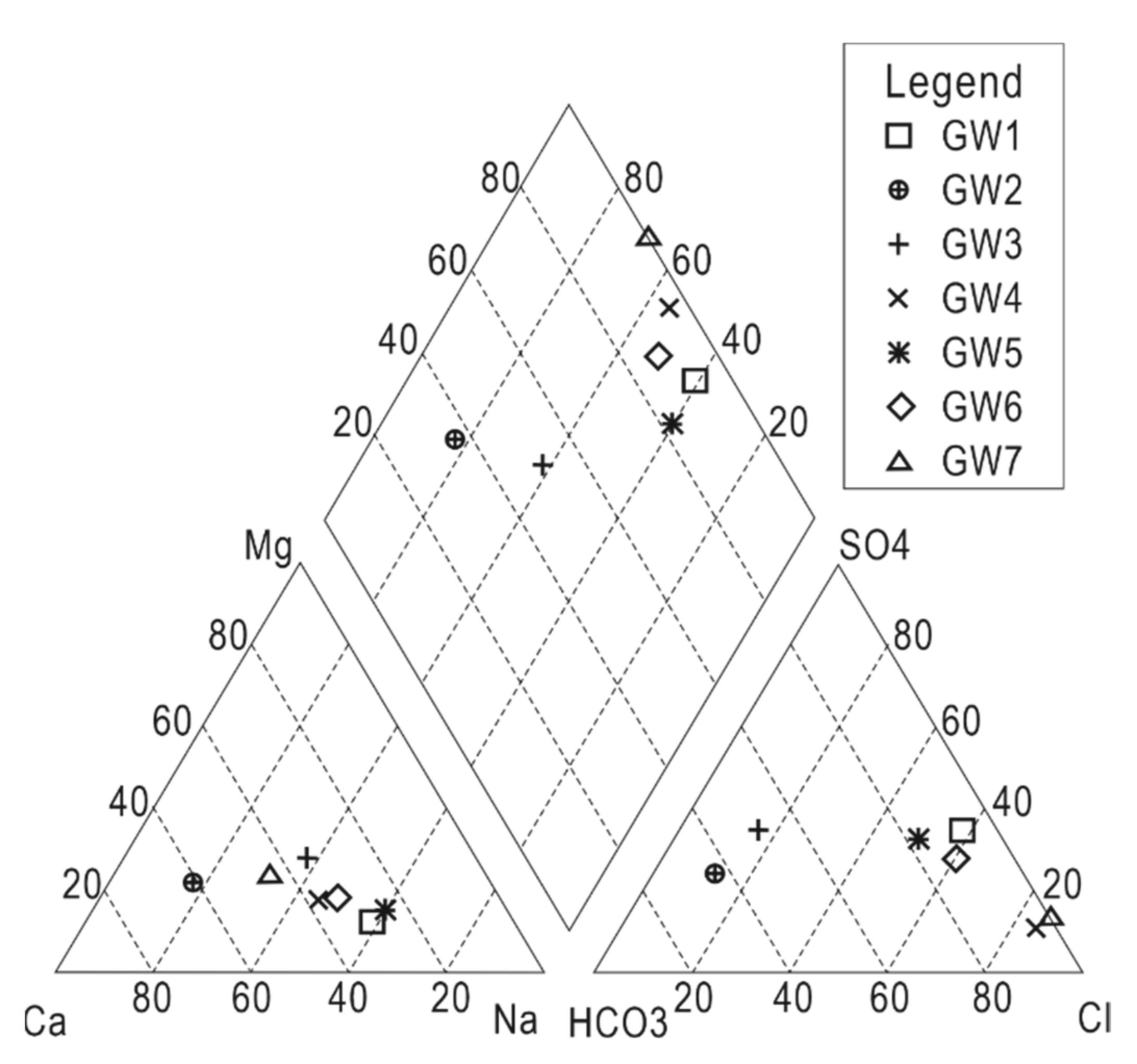
3.4. Hydrochemical Verification

The test results of the groundwater monitoring wells are shown in Table 4 and the pollutant distribution map was drawn according to these test results, as shown in Figure 7.
According to the test results, the concentrations of trans-1,2-dichloroethylene, 1,2,3-trichlorobenzene, and hexachlorocyclohexane were all higher than the standard (National Standards of the People’s Republic of China: Standard for groundwater quality (GB/T 14848-2017). (This standard will be used in the rest of the article). Trans-1,2-dichloroethylene was mainly concentrated in GW1, GW4. The water of GW4 (61.3 μg/L) and GW1 (703 μg/L) was beyond level V, which means the pollution was very heavy. GW1, GW3, GW4, GW7, GW8 all displayed high concentrations of 1,2,3-trichlorobenzene. GW1 (23 μg/L), GW3 (41.2 μg/L), GW7 (103 μg/L), GW8 (102 μg/L) were level IV, and GW4 (316 μg/L) was level V. Hexachlorocyclohexane gathered in GW3, GW4, GW7, and GW8. The highest concentration was GW7 (708 μg/L), which was level V. GW3 (13 μg/L), GW4 (72 μg/L), GW8 (65 μg/L) were all level IV. The whole study field was polluted and needs remediation.
The water sample test results show that the groundwater at the site was mainly composed of three pollutants: trans-1,2-dichloroethylene, 1,2,3-trichlorobenzene, and hexachlorocyclohexane. Due to the limited number of wells, there were some errors in the detection of contaminant distributions across the site. Nevertheless, the overall trend was correct. The HCH concentrations were highest near GW7 and the trans-1,2-dichloroethylene concentrations were highest near GW1. Overall, when the groundwater flowed upstream, the concentration of pollutants dropped sharply, so the concentration of pollutants near GW12 was 0.
The main pollutant near GW7 was hexachlorocyclohexane, which could be due to a leakage occurring in the production process of hexachlorocyclohexane. The total highest concentration was 783 μg/L. Furthermore, the resistivity of the groundwater reached 1131.222 Ω·m and 2840.909 Ω·m in June 2018 and April 2019, respectively, which also illustrates the high concentration of pollution in groundwater. It diffused mainly in the southeast direction, along with the groundwater flow, and the concentration in the southwest region was basically zero. Probably due to the overall detection depth of ML-I being too shallow and in parallel with the groundwater flow direction, only the 25–33 m region at a 3 m depth showed contamination. The area of 0–20 m on the ML-II profile, with more than 500 Ω·m resistivity, could be the remains of the acid tank. The east of acid tank was more than 150 Ω·m. This could be caused by a high concentration of HCH. We suspected that there was another source to the west of the HCH production building (Figure 6). Theoretically, pollutants are most concentrated near to the source and then spread out. Pollutant concentrations decline most slowly downstream of groundwater flows, while concentrations decline rapidly upstream of groundwater flows. On the profile ML-II, this anomaly could be observed. Due to the lack of sufficient observation wells, the contaminant concentrations were the result of interpolation calculations and were not reliable within the northwest of the site. At the same time, combined with the flow direction of the groundwater, there could be a source of pollution or a leak from the acid tank itself upstream of the anomaly, i.e., in the northwest direction, which could result in the anomaly. Unfortunately, we were not able to carry out further verification.
Overall, profile ML-III and profile ML-IV were highly resistant. Near the two profiles, a high concentration of trans-1,2-dichloroethylene was detected in the groundwater of well GW1. The maximum value of trans-1,2-dichloroethylene detected in GW1 was 703 μg/L and the concentration decreased toward the northeast. This was close to the semi-outdoor unloading platform and could be caused by the leakage of raw materials during loading, unloading, and transportation. According to existing experimental results and the actual site application analysis, most organic pollution is often insoluble in water and has a high electrical resistivity [35]. Pollutants penetrate downward into the groundwater under the action of their own weight. Due to the adsorption of the soil, they often adhere to the soil surface and fill the soil pores. Then, they obstruct the passage of free water, which leads to an increase in soil resistivity. When the pollutants enter the groundwater, some are affected by the flow of water and diffuse downstream. The other part of the pollutants is adsorbed onto the medium, prompting the area to show an abnormally high resistivity. Meanwhile, trans-1,2-dichloroethylene is a liquid organic compound with high volatility. The high-resistivity region within the profiles could be a mixture of the volatile phase and the liquid phase of anti-1,2-dichloroethylene. Combined with what has already been reported, volatile organics could lead to an increase in resistance.
The overall concentration of 1,2,3-trichlorobenzene was relatively low, reaching a maximum of 316 μg/L in the groundwater, and the resistivity of the groundwater reached 3984.064 Ω·m in GW4, which could be due to convective dispersion in the southeast direction. According to the map of the factory, we could not explain the source of pollution. We thought that it was caused by the trichlorobenzene production workshop on the west side of the plant. As a result of the abnormity of the ERT result, we found new pollution in the field and tried to identify its source.

4. Conclusions

ERT is a widely used method in geophysics that can effectively investigate underground areas. It is employed cost effectively for the non-intrusive and remote investigation of contaminated sites, including the investigation of pollution sources and pollutant distribution, at high speed, efficiently, and on various scales. In this paper, ERT was used to detect the pollution plumes of organochlorine pesticides in the soil and groundwater within the local area of a pesticide plant in northeastern China. Extensive remote sensing data were obtained from the site investigations. Validated by the actual sampling and analytical data from six monitoring wells, we verified that ERT could characterize the pollution areas well. The abnormity of ERT results indicated the pollution extent based on the spatial scale at the site. In this study, we unexpectedly found a new pollution source and demonstrated a useful remote sensing technology for the more accurate detection of plume sources. This confirmed that ERT has a good applicability for the investigation of contaminated sites. It can provide effective information to support evaluation and restoration strategies. The quantitative relationship between pollutant concentration and resistivity still needs further field- and lab-based studies due to the complex factors of the subsurface environment.

Author Contributions

Conceptualization, Z.Y. and X.S.; methodology, Z.Y.; software, Z.Y.; validation, Z.Y., X.S., and C.G.; formal analysis, C.G.; investigation, Z.Y. and Y.W. (Yunlong Wang); resources, Y.W. (Yunlong Wang); data curation, Y.W. (Yuhui Wu); writing—original draft preparation, Z.Y.; writing—review and editing, Y.Y., X.S., and Y.W. (Yuhui Wu); visualization, Z.Y.; supervision, Y.Y.; project administration, Y.Y.; funding acquisition, Y.Y. All authors have read and agreed to the published version of the manuscript.

Funding

This research was funded by the National Major R&D Program of China (no. 2019YFC1804800), the Major R&D Project of Liaoning Province (no. 2020JH2/10300083), and the 111 Project (B16020) of Jilin University, China.

Institutional Review Board Statement

Not applicable.

Informed Consent Statement

Not applicable.

Conflicts of Interest

The authors declare no conflict of interest.

References

  1. Ghimire, N.; Woodward, R.T. Under- And over-Use of Pesticides: An International Analysis. Ecol. Econ. 2013, 89, 73–81. [Google Scholar] [CrossRef]
  2. Rafique, N.; Tariq, S.R. Distribution and Source Apportionment Studies of Heavy Metals in Soil of Cotton/Wheat Fields. Environ. Monit. Assess. 2016, 188, 309. [Google Scholar] [CrossRef] [PubMed]
  3. Shternshis, M.V.; Belyaev, A.A.; Matchenko, N.S.; Shpatova, T.V.; Lelyak, A.A. Possibility of Biological Control of Primocane Fruiting Raspberry Disease Caused by Fusarium Sambucinum. Environ. Sci. Pollut. Res. 2015, 22, 15656–15662. [Google Scholar] [CrossRef] [PubMed]
  4. Liu, J.P.; Fang, J.; Wei, G. Compressed Sensing Reconstruction Algorithm Based on DCT Band Energy. J. S. China Univ. Technol. 2015, 43, 28–33. [Google Scholar]
  5. Marín-Benito, J.M.; Sánchez-Martín, M.J.; Rodríguez-Cruz, M.S. Impact of Spent Mushroom Substrates on the Fate of Pesticides in Soil, and Their Use for Preventing and/or Controlling Soil and Water Contamination: A Review. Toxics 2016, 4, 17. [Google Scholar] [CrossRef] [Green Version]
  6. Oerke, E.C. Crop Losses to Pests. J. Agric. Sci. 2006, 144, 31–43. [Google Scholar] [CrossRef]
  7. Niu, L.; Xu, C.; Yao, Y.; Liu, K.; Yang, F.; Tang, M.; Liu, W. Status, Influences and Risk Assessment of Hexachlorocyclohexanes in Agricultural Soils Across China. Environ. Sci. Technol. 2013, 47, 12140–12147. [Google Scholar] [CrossRef]
  8. Sun, Y.; Chang, X.; Zhao, L.; Zhou, B.; Weng, L.; Li, Y. Comparative Study on the Pollution Status of Organochlorine Pesticides (OCPs) and Bacterial Community Diversity and Structure between Plastic Shed and Open-Field Soils from Northern China. Sci. Total Environ. 2020, 741, 139620. [Google Scholar] [CrossRef]
  9. Wong, C.S.; Garrison, A.W.; Foreman, W.T. Enantiomeric Composition of Chiral Polychlorinated Biphenyl Atropisomers in Aquatic Bed Sediment. Environ. Sci. Technol. 2001, 35, 33–39. [Google Scholar] [CrossRef]
  10. Shang, X.; Dong, G.; Zhang, H.; Zhang, L.; Yu, X.; Li, J.; Wang, X.; Yue, B.; Zhao, Y.; Wu, Y. Polybrominated Diphenyl Ethers (PBDEs) and Indicator Polychlorinated Biphenyls (PCBs) in Various Marine Fish from Zhoushan Fishery, China. Food Control 2016, 67, 240–246. [Google Scholar] [CrossRef]
  11. Briz, V.; Molina-Molina, J.M.; Sánchez-Redondo, S.; Fernández, M.F.; Grimalt, J.O.; Olea, N.; Rodríguez-Farré, E.; Suñol, C. Differential Estrogenic Effects of the Persistent Organochlorine Pesticides Dieldrin, Endosulfan, and Lindane in Primary Neuronal Cultures. Toxicol. Sci. 2011, 120, 413–427. [Google Scholar] [CrossRef] [PubMed]
  12. Gao, J.; Zhou, H.; Pan, G.; Wang, J.; Chen, B. Factors Influencing the Persistence of Organochlorine Pesticides in Surface Soil from the Region around the Hongze Lake, China. Sci. Total Environ. 2013, 443, 7–13. [Google Scholar] [CrossRef] [PubMed]
  13. Naqvi, S.M.; Vaishnavi, C. Bioaccumulative Potential and Toxicity of Endosulfan Insecticide to Non-Target Animals. Comp. Biochem. Physiol. C Comp. Pharmacol. 1993, 105, 347–361. [Google Scholar] [CrossRef]
  14. Kalra, S.; Dewan, P.; Batra, P.; Sharma, T.; Tyagi, V.; Banerjee, B.D. Organochlorine Pesticide Exposure in Mothers and Neural Tube Defects in Offsprings. Reprod. Toxicol. 2016, 66, 56–60. [Google Scholar] [CrossRef] [PubMed]
  15. Kim, K.H.; Kabir, E.; Jahan, S.A. Exposure to Pesticides and the Associated Human Health Effects. Sci. Total Environ. 2017, 575, 525–535. [Google Scholar] [CrossRef]
  16. Ramakrishnan, B.; Venkateswarlu, K.; Sethunathan, N.; Megharaj, M. Local Applications but Global Implications: Can Pesticides Drive Microorganisms to Develop Antimicrobial Resistance. Sci. Total Environ. 2019, 654, 177–189. [Google Scholar] [CrossRef]
  17. Abdo, W.; Hirata, A.; Sakai, H.; El-Sawak, A.; Nikami, H.; Yanai, T. Combined Effects of Organochlorine Pesticides Heptachlor and Hexachlorobenzene on the Promotion Stage of Hepatocarcinogenesis in Rats. Food Chem. Toxicol. 2013, 55, 578–585. [Google Scholar] [CrossRef]
  18. Ennour-Idrissi, K.; Ayotte, P.; Diorio, C. Persistent Organic Pollutants and Breast Cancer: A Systematic Review and Critical Appraisal of the Literature. Cancers 2019, 11, 1063. [Google Scholar] [CrossRef] [Green Version]
  19. Mathur, V.; Bhatnagar, P.; Sharma, R.G.; Acharya, V.; Sexana, R. Breast Cancer Incidence and Exposure to Pesticides among Women Originating from Jaipur. Environ. Int. 2002, 28, 331–336. [Google Scholar] [CrossRef]
  20. Rathore, M.; Bhatnagar, P.; Mathur, D.; Saxena, G.N. Burden of Organochlorine Pesticides in Blood and Its Effect on Thyroid Hormones in Women. Sci. Total Environ. 2002, 295, 207–215. [Google Scholar] [CrossRef]
  21. Ennaceur, S.; Gandoura, N.; Driss, M.R. Distribution of Polychlorinated Biphenyls and Organochlorine Pesticides in Human Breast Milk from Various Locations in Tunisia: Levels of Contamination, Influencing Factors, and Infant Risk Assessment. Environ. Res. 2008, 108, 86–93. [Google Scholar] [CrossRef] [PubMed]
  22. Porter, S.N.; Humphries, M.S.; Buah-Kwofie, A.; Schleyer, M.H. Accumulation of Organochlorine Pesticides in Reef Organisms from Marginal Coral Reefs in South Africa and Links with Coastal Groundwater. Mar. Pollut. Bull. 2018, 137, 295–305. [Google Scholar] [CrossRef] [PubMed]
  23. Wu, C.; Luo, Y.; Gui, T.; Huang, Y. Concentrations and Potential Health Hazards of Organochlorine Pesticides in Shallow Groundwater of Taihu Lake Region, China. Sci. Total Environ. 2014, 470–471, 1047–1055. [Google Scholar] [CrossRef] [PubMed]
  24. Zhang, C.; Liao, X.; Li, J.; Xu, L.; Liu, M.; Du, B.; Wang, Y. Influence of Long-Term Sewage Irrigation on the Distribution of Organochlorine Pesticides in Soil–Groundwater Systems. Chemosphere 2013, 92, 337–343. [Google Scholar] [CrossRef] [PubMed]
  25. Derbalah, A.; Chidya, R.; Jadoon, W.; Sakugawa, H. Temporal Trends in Organophosphorus Pesticides Use and Concentrations in River Water in Japan, and Risk Assessment. J. Environ. Sci. 2019, 79, 135–152. [Google Scholar] [CrossRef]
  26. El-Nahhal, I. Pesticide Residues in Drinking Water, Their Potential Risk to Human Health and Removal Options. J. Environ. Manag. 2021, 299, 113611. [Google Scholar] [CrossRef]
  27. IPEP. International POPs Elimination Project. Fostering Active and Efficient Civil Society Participation in Preparation for Implementation of the Stockholm Convention, Country Situation on Persistent Organic Pollutants (POPs) in India; Toxics Link: New Delhi, India, 2006; pp. 1–57. [Google Scholar]
  28. Liu, Y.; Bashir, S.; Stollberg, R.; Trabitzsch, R.; Weiß, H.; Paschke, H.; Nijenhuis, I.; Richnow, H.-H. Compound Specific and Enantioselective Stable Isotope Analysis as Tools to Monitor Transformation of Hexachlorocyclohexane (HCH) in a Complex Aquifer System. Environ. Sci. Technol. 2017, 51, 8909–8916. [Google Scholar] [CrossRef]
  29. Atekwana, E.A.; Atekwana, E.A. Geophysical Signatures of Microbial Activity at Hydrocarbon Contaminated Sites: A Review. Surv. Geophys. 2010, 31, 247–283. [Google Scholar] [CrossRef]
  30. Simyrdanis, K.; Papadopoulos, N.; Soupios, P.; Kirkou, S.; Tsourlos, P. Characterization and Monitoring of Subsurface Contamination from Olive Oil Mills’ Waste Waters Using Electrical Resistivity Tomography. Sci. Total Environ. 2018, 637–638, 991–1003. [Google Scholar] [CrossRef]
  31. Delaney, A.J.; Peapples, P.R.; Arcone, S.A. Electrical Resistivity of Frozen and Petroleum-Contaminated Fine-Grained Soil. Cold Reg. Sci. Technol. 2001, 32, 107–119. [Google Scholar] [CrossRef]
  32. Cardarelli, E.; Di Filippo, G. Electrical Resistivity and Induced Polarization Tomography in Identifying the Plume of Chlorinated Hydrocarbons in Sedimentary Formation: A Case Study in Rho (Milan—Italy). Waste Manag. Res. 2009, 27, 595–602. [Google Scholar] [CrossRef] [PubMed]
  33. Orlando, L.; Renzi, B. Electrical Permittivity and Resistivity Time Lapses of Multiphase DNAPLs in a Lab Test. Water Resour. Res. 2015, 51, 377–389. [Google Scholar] [CrossRef]
  34. Cassidy, N.J. Evaluating LNAPL Contamination Using GPR Signal Attenuation Analysis and Dielectric Property Measurements: Practical Implications for Hydrological Studies. J. Contam. Hydrol. 2007, 94, 49–75. [Google Scholar] [CrossRef] [PubMed]
  35. Wang, T.-P.; Chen, C.-C.; Tong, L.-T.; Chang, P.-Y.; Chen, Y.-C.; Dong, T.-H.; Liu, H.-C.; Lin, C.-P.; Yang, K.-H.; Ho, C.-J.; et al. Applying FDEM, ERT and GPR at a Site with Soil Contamination: A Case Study. J. Appl. Geophys. 2015, 121, 21–30. [Google Scholar] [CrossRef]
  36. Hudson, E.; Kulessa, B.; Edwards, P.; Williams, T.; Walsh, R. Integrated Hydrological and Geophysical Characterisation of Surface and Subsurface Water Contamination at Abandoned Metal Mines. Water Air Soil Pollut. 2018, 229, 256. [Google Scholar] [CrossRef] [Green Version]
  37. Vásconez-Maza, M.D.; Martínez-Segura, M.A.; Bueso, M.C.; Faz, Á.; García-Nieto, M.C.; Gabarrón, M.; Acosta, J.A. Predicting Spatial Distribution of Heavy Metals in an Abandoned Phosphogypsum Pond Combining Geochemistry, Electrical Resistivity Tomography and Statistical Methods. J. Hazard. Mater. 2019, 374, 392–400. [Google Scholar] [CrossRef]
  38. Pujari, P.R.; Pardhi, P.; Muduli, P.; Harkare, P.; Nanoti, M.V. Assessment of Pollution Near Landfill Site in Nagpur, India by Resistivity Imaging and GPR. Environ. Monit. Assess. 2007, 131, 489–500. [Google Scholar] [CrossRef]
  39. Bichet, V.; Grisey, E.; Aleya, L. Spatial Characterization of Leachate Plume Using Electrical Resistivity Tomography in a Landfill Composed of Old and New Cells (Belfort, France). Eng. Geol. 2016, 211, 61–73. [Google Scholar] [CrossRef]
  40. Azizi, F.; Vadiati, M.; Asghari Moghaddam, A.; Nazemi, A.; Adamowski, J. A Hydrogeological-Based Multi-Criteria Method for Assessing the Vulnerability of Coastal Aquifers to Saltwater Intrusion. Environ. Earth Sci. 2019, 78, 548. [Google Scholar] [CrossRef]
  41. Maury, S.; Balaji, S. Application of Resistivity and GPR Techniques for the Characterization of the Coastal Litho-Stratigraphy and Aquifer Vulnerability Due to Seawater Intrusion. Estuar. Coast. Shelf Sci. 2015, 165, 104–116. [Google Scholar] [CrossRef]
  42. Shao, S.; Gao, C.; Guo, X.; Wang, Y.; Zhang, Z.; Yu, L.; Tang, H. Mapping the Contaminant Plume of an Abandoned Hydrocarbon Disposal Site with Geophysical and Geochemical Methods, Jiangsu, China. Environ. Sci. Pollut. Res. 2019, 26, 24645–24657. [Google Scholar] [CrossRef] [PubMed]
  43. Zhan, L.; Xu, H.; Jiang, X.; Lan, J.; Chen, Y.; Zhang, Z. Use of Electrical Resistivity Tomography for Detecting the Distribution of Leachate and Gas in a Large-Scale MSW Landfill Cell. Environ. Sci. Pollut. Res. 2019, 26, 20325–20343. [Google Scholar] [CrossRef] [PubMed]
  44. Carretero, S.; Rapaglia, J.; Perdomo, S.; Albino Martínez, C.; Rodrigues Capítulo, L.; Gómez, L.; Kruse, E. A Multi-Parameter Study of Groundwater–Seawater Interactions along Partido de La Costa, Buenos Aires Province, Argentina. Environ. Earth Sci. 2019, 78, 513. [Google Scholar] [CrossRef]
  45. Alesse, B.; Orlando, L.; Palladini, L. Non-invasive Lab Test in the Monitoring of Vadose Zone Contaminated by Light Non-aqueous Phase Liquid. Geophys. Prospect. 2019, 67, 2161–2175. [Google Scholar] [CrossRef]
  46. Wang, Y. Study on Numerical Simulation and Inversion of Electrical Resistivity Method for Heavy Metal Contaminated Sites; China University of Mining & Technology: Beijing, China, 2013. (In Chinese) [Google Scholar]
  47. Rosales, R.M.; Martínez-Pagan, P.; Faz, A.; Moreno-Cornejo, J. Environmental Monitoring Using Electrical Resistivity Tomography (ERT) in the Subsoil of Three Former Petrol Stations in SE of Spain. Water Air Soil Pollut. 2012, 223, 3757–3773. [Google Scholar] [CrossRef]
  48. Raji, W.O.; Obadare, I.G.; Odukoya, M.A.; Johnson, L.M. Electrical Resistivity Mapping of Oil Spills in a Coastal Environment of Lagos, Nigeria. Arab. J. Geosci. 2018, 11, 144. [Google Scholar] [CrossRef]
  49. Caterina, D.; Flores Orozco, A.; Nguyen, F. Long-Term ERT Monitoring of Biogeochemical Changes of an Aged Hydrocarbon Contamination. J. Contam. Hydrol. 2017, 201, 19–29. [Google Scholar] [CrossRef]
  50. Yang, C.; You, J. High Resistivities Associated with an LNAPL Plume Imaged by Geoelectrical Tomography. In Proceedings of the SEG Technical Program Expanded Abstracts 1999; Society of Exploration Geophysicists: Houston, TX, USA, 1999; pp. 469–472. [Google Scholar]
  51. Lago, A.L.; Elis, V.R.; Borges, W.R.; Penner, G.C. Geophysical Investigation Using Resistivity and GPR Methods: A Case Study of a Lubricant Oil Waste Disposal Area in the City of Ribeirão Preto, São Paulo, Brazil. Environ. Geol. 2009, 58, 407–417. [Google Scholar] [CrossRef]
  52. Wang, Y.; Anderson, N.; Torgashov, E. Condition Assessment of Building Foundation in Karst Terrain Using Both Electrical Resistivity Tomography and Multi-Channel Analysis Surface Wave Techniques. Geotech. Geol. Eng. 2019, 38, 1839–1855. [Google Scholar] [CrossRef]
  53. Heenan, J.; Slater, L.D.; Ntarlagiannis, D.; Atekwana, E.A.; Fathepure, B.Z.; Dalvi, S.; Ross, C.; Werkema, D.D.; Atekwana, E.A. Electrical Resistivity Imaging for Long-Term Autonomous Monitoring of Hydrocarbon Degradation: Lessons from the Deepwater Horizon Oil Spill. Geophysics 2015, 80, B1–B11. [Google Scholar] [CrossRef]
  54. Pan, Y.; Jia, Y.; Xu, Z.; Lei, X. The study on resistivity characteristics of oil contaminated soil in different influencing factors. Acta Sci. Circumst. 2015, 35, 880–889. (In Chinese) [Google Scholar]
Figure 1. Schematic diagrams for (a) the original plant layout, survey line distribution, and sampling well distribution; (b) the north–south hydrogeological cross-section of the site and stratum description.
Applsci 12 02816 g001
Figure 2. A piper diagram for the groundwater geochemistry at the site.
Applsci 12 02816 g002
Figure 3. A conceptual model of the remote high-density electrical detection.
Applsci 12 02816 g003
Figure 4. The site resistivity background value that was used as reference setting for further work.
Applsci 12 02816 g004
Figure 5. The ERT inversion results of the remote investigations along different measuring lines (Line I-IV).
Applsci 12 02816 g005
Figure 6. The ERT profiles of the pollution plume distribution.
Applsci 12 02816 g006
Figure 7. A schematic diagram of the concentration distribution of organic pollutants in the groundwater: (a) the concentration distribution of trans-1,2-dichloroethylene; (b) the concentration distribution of trans-1,2-dichloroethylene; (c) the concentration distribution of hexachlorocyclohexane.
Applsci 12 02816 g007
Table 1. The resistivity ranges of common materials.
ExperimentApplication
MaterialResistivity (Ω·m)LocationGeological
Material
Resistivity (Ω·m)References
Lower BoundUpper Bound
Clay1 [46]100 1“El Trampolin” Petrol StationPredominantly silts of reddish to brown shades.0–50[47]
Sand4 1800 1Ijegun Community of Lagos NigeriaSand layer120–328[48]
Loam5 150 1Oil leakage in underground tanks in Liège (Belgium).Quaternary clayey and loamy soils<20[49]
Shale20 12000 1Ijegun Community of Lagos NigeriaShale/mudstone layer25–116[48]
Gravel/conglomerate2000 1104 1LNAPL leak from an underground pipelineGravel layer170–250[50]
Coarse sandstone10 19.6 × 10⁴ 1“Lebor Campsa” Petrol Station in the southeast of the Iberian PeninsulaQuaternary alluviums (gravel, sand, and clay)70–350[47]
Siltstone1 11.5 × 10⁴ 1------------
Sandstone50 18.0 × 10³ 1A lubricant oil waste disposal area in BrazilReddish sandstone layers, fine to medium, with well selected frosted grains, highly spherical185–3000[51]
Limestone80 11.0 × 10³ 1In foundation survey projects for hotel buildings in KentuckyLimestone<60 (identified where the moisture content was high)[52]
1 Data adapted from ref [46]. 2013 Wang, Y.
Table 2. The resistivity of the water samples.
WellGroundwater Resistivity (Ω·m)
June 2018April 2019
GW16.0536.536
GW232.78715.221
GW329.07013.477
GW43984.064---
GW68.104---
GW71131.2222840.909
Note: “---”: Some wells’ data are missing.
Table 3. Profile details.
Profile NumberDeviceLayered Power SupplyPower Supply TimeTotal Number of ElectrodesElectrode DistanceRepeated Collection TimesTotal Data Points
ML-IWenner-AlphaNo1 s242384
ML-IIWenner-AlphaNo1 s4023235
ML-IIIWenner-AlphaNo1 s243384
ML-IVWenner-AlphaNo1 s3243155
Table 4. The monitoring results of water samples, unit: μg/L.
Groundwater WellTrans-1,2-Dichloroethylene1,2,3-TrichlorobenzeneHexachlorocyclohexane
GW1703231
GW21.1<1.00
GW31.741.213
GW461.331672
GW79.4103783
GW85.510265
Publisher’s Note: MDPI stays neutral with regard to jurisdictional claims in published maps and institutional affiliations.

