A Dynamic Procedure for Time and Space Domain Based on Differential Cubature Principle

Abstract

Based on the differential cubature (DC) principle, a dynamic procedure for simultaneous discretization of time and space is developed. A spatial–temporal differential cubature analysis method for dynamic problems is established with the Timoshenko shear beam; the reliability of analysis results obtained by which is verified, and the stability of the numerical scheme is studied. This method is extended to the two-dimensional structure, and the forced vibration analysis is carried out with the thin plate as an example. The research shows that the method can acquire highly accurate numerical results, and the calculated time-history numerical solution of beam displacement is extremely consistent with the analytical solution, which can adopt to the changes in beam properties and load parameters. With fewer nodes and longer time step than the finite element method (FEM), the method in this paper can still obtain stable and accurate results when solving displacement responses of plate under forced vibration. The numerical stability of this method is closely related to the grid form and the size of time step, and the increase in the number of nodes in the time domain is conducive to increasing the stability range.

1. Introduction

Structural dynamic analysis generally refers to calculating the response of the structure according to the known structure and dynamic load, so as to determine the bearing capacity and dynamic characteristics of the structure, and ultimately provide a reasonable basis for structural design. Traditional dynamic analysis methods can be divided into two categories: one is based on coordinate transformation [1,2], such as mode superposition method, frequency domain method, etc; and another kind of direct solution method for dynamic differential equations can continue to be divided into display difference method and implicit progressive integration method [3,4,5]. These analysis methods have certain application scope. For instance, the mode superposition method is only applicable to linear and time-invariant systems. The display difference method as a conditionally stable method requires strict control of the analysis step distance. Although the implicit step-by-step integration method is unconditionally stable, it will bring great computational consumption when the degree of freedom is large. Therefore, in order to cope with the large and complex structure in practical engineering and meet the accuracy requirements, it is necessary to develop a more efficient and high-precision dynamic analysis method.

Differential quadrature method (DQM) [6,7,8,9] is a numerical method for solving differential equations proposed in the 1970s and developed in recent years. The method has the advantages of small amounts of calculation, high precision, and simple operation. Fung [10,11] first applied the DQ method to solve the initial value problem, and then many scholars [12,13,14,15,16] carried out deeper research in this area, forming the DQ dynamic analysis method. Since the high-order discretization method is also used in the time domain, high precision and very stable results can be obtained by the method. Despite its many advantages, the DQM is only suitable for the regular region formed by orthogonal superposition of multiple one-dimensional directions. To cope with this limitation, Civan proposed the differential cubature method (DCM) [17,18] based on the theory of multivariate interpolation approximation, and later researchers [19,20,21,22] mainly applied it to the boundary value problems in two-dimensional space domain, such as the natural frequency, bending, buckling analysis of plate and shell, and the transfer of steady-state space and convection diffusion. Wu [23,24,25] applied the DCM to analyze the free vibration of circular plate, curved beam, and medium-thick plate considering shear effect, and obtained high-precision results by using fewer nodes. Hajmohammad [26] first analyzed the dynamic response of composite plates by DCM combined with the Newmark method, and then other scholars made similar applications. Bendarma [27] analyzed the mechanical characteristics and dynamic behavior of fiberglass composite material structure used for perforation tests based on experimental results. Compeán et al. [28] analyzed the characterization and stability of a multivariable milling tool by enhanced multistage homotopy perturbation method. Although the analysis of dynamic response has been carried out in the existing literature on the application of DCM, due to the different calculation methods used in space domain and time domain, the functional connection between time and space is cut off, which indicates that these measures also belong to the processing method of space–time separation. In order to realize the precision matching between space domain and time domain, this paper combines space domain and time domain into space domain based on DCM, which combines time dimension and space dimension into the same grid, and then solves the equations after space–time discretization. The vibration problem of Timoshenko shear beam is selected to illustrate the space–time dynamic analysis method, and its stability and influencing factors are analyzed. In addition, in order to expand the spatial dimension of the spatio–temporal dynamic analysis method, the response analysis of the forced vibration of the thin plate is carried out based on the three-dimensional DCM, and evaluated its accuracy and computational efficiency by comparing the finite element solutions.

2. Basic Principles of the DCM

The DC method is used to obtain the derivative value at a discrete point based on the multivariate function approximation. Its basic idea is to approximate the arbitrary order partial derivative value of a multivariate continuous function at a given point to the linear weighted sum of all discrete function values in the entire domain. For a binary function, assuming that there is a total of N discrete points in the two-dimensional domain, the partial derivatives of the functions at the given discrete points can be written uniformly as

$$\Re \left(f(x,y)\right)={\{\Re [f(x,y)]\}}_i\approx {\displaystyle \sum _{j=1}^N{c}_{ij}f(x_j,y_j)},\hspace{1em}i=1, 2, \cdots , N$$

(1)

where $\Re$ represents the differential operator of any order partial derivative of the specified variable or the mixed partial derivative of different variables, (x_j,y_j) and f(x_j,y_j), respectively, represent the coordinates of the j-th discrete point, and the corresponding function value, c_ij, is the DC weight coefficient of the operator L. Regarding this weight coefficient c_ij, it can be obtained by the following expression:

$$\mathit{c}=\Re [\mathit{\phi }]{\mathit{\phi }}^{-1}=\left[\begin{array}{cccc}{c}_{11}& c_{12}& \cdots & c_{1N}\\ c_{21}& c_{22}& \cdots & c_{2N}\\ ⋮& ⋮& \ddots & ⋮\\ c_{N1}& c_{N2}& \cdots & c_{NN}\end{array}\right],$$

(2)

where

$$\Re [\mathit{\phi }]=\left[\begin{array}{cccc}\Re ({\phi }_{11})& \Re ({\phi }_{12})& \cdots & \Re ({\phi }_{1N})\\ \Re ({\phi }_{21})& \Re ({\phi }_{22})& \cdots & \Re ({\phi }_{2N})\\ ⋮& ⋮& \ddots & ⋮\\ \Re ({\phi }_{N1})& \Re ({\phi }_{N2})& \cdots & \Re ({\phi }_{NN})\end{array}\right],$$

where $\phi$ is a binary basis function in the N-dimensional vector space, and the natural basis function is selected here. c is called the DC weight coefficient matrix, and Equation (2) is also the implicit solution method of DC weight coefficient.

3. Space—Time Dynamic Analysis Method Based on DCM

3.1. Dynamic Equation and Initial and Boundary Conditions

A one-dimensional Timoshenko shear beam is selected as the analysis object. The dynamic governing equation under general dynamic load F(x,t) is

$$EI\frac{{\partial }^{4}y}{\partial x^4}+\rho \frac{{\partial }^{2}y}{\partial t^2}-\rho \zeta \frac{{\partial }^{4}y}{\partial x^2\partial t^2}=F(x,t)$$

(3)

where x and t represent the coordinates of space and time, respectively. y represents lateral displacement. The range of x is [0, L], and the range of t is [0, T]. L is beam length, T is external load duration, EI is distributed stiffness. ρ is the distribution mass, and ζ is the shear influence parameters, of which the dimension is the quadratic of length.

For the convenience of discretizing the equation, let ξ = x/L, τ = t/T, dimensionless Equation (1) into

$$\frac{EI}{L^4}\frac{{\partial }^{4}y}{\partial {\xi }^4}+\frac{\rho }{T^2}\frac{{\partial }^{2}y}{\partial {\tau }^2}-\frac{\rho \zeta }{T^2{L}^2}\frac{{\partial }^{4}y}{\partial {\xi }^2\partial {\tau }^2}=F(L\xi ,T\tau )$$

(4)

Assuming that both ends of the beam are simply supported, the boundary conditions are

$${(y)}_{\xi =0,1}=0$$

(5)

$${\left(\frac{{\partial }^{2}y}{\partial {\xi }^2}\right)}_{\xi =0,1}=0$$

(6)

The initial condition is

$${(y)}_{\tau =0}=y_0$$

(7)

$${\left(\frac{\partial y}{\partial \tau }\right)}_{\tau =0}={\dot{y}}_0$$

(8)

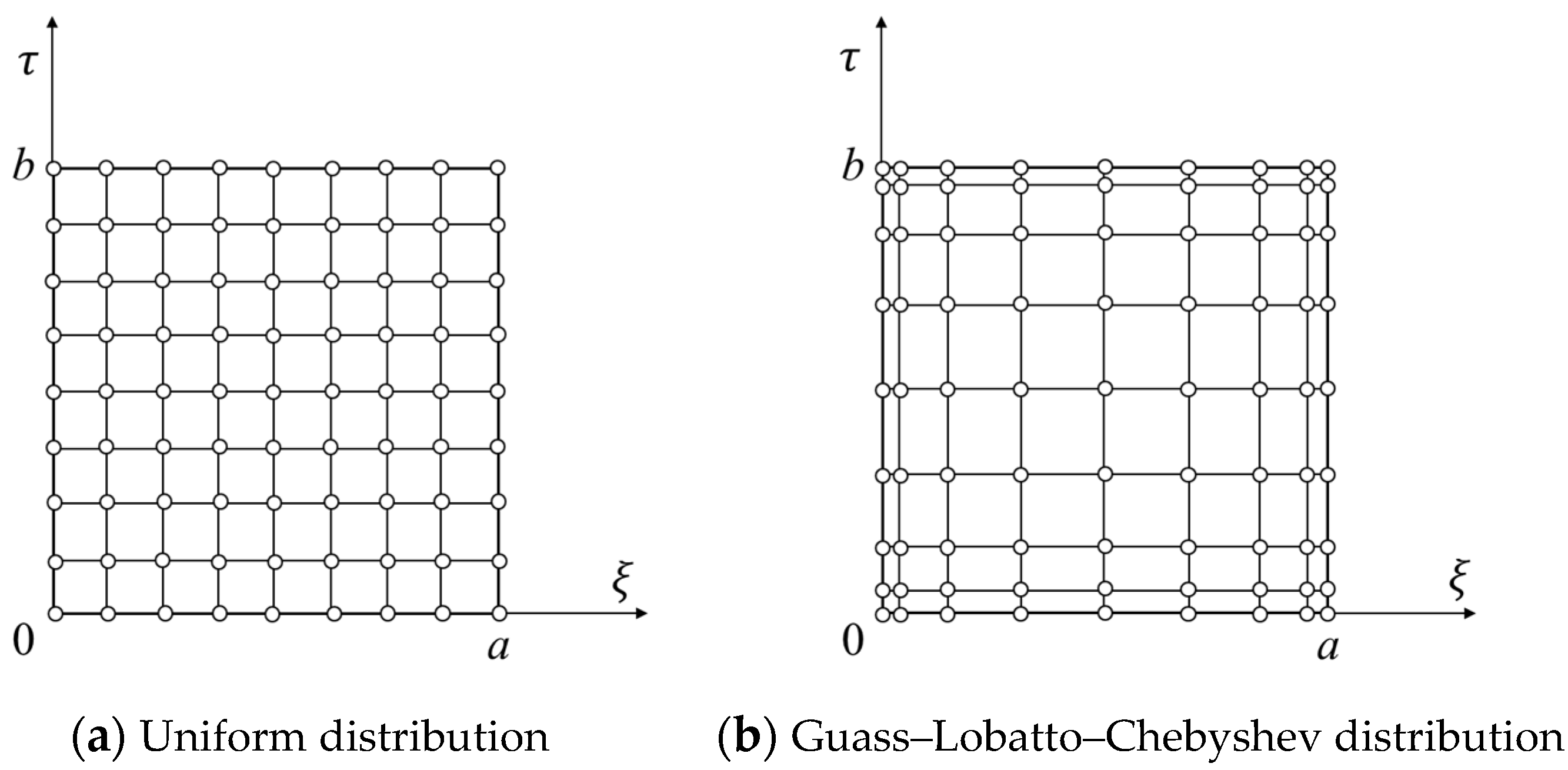
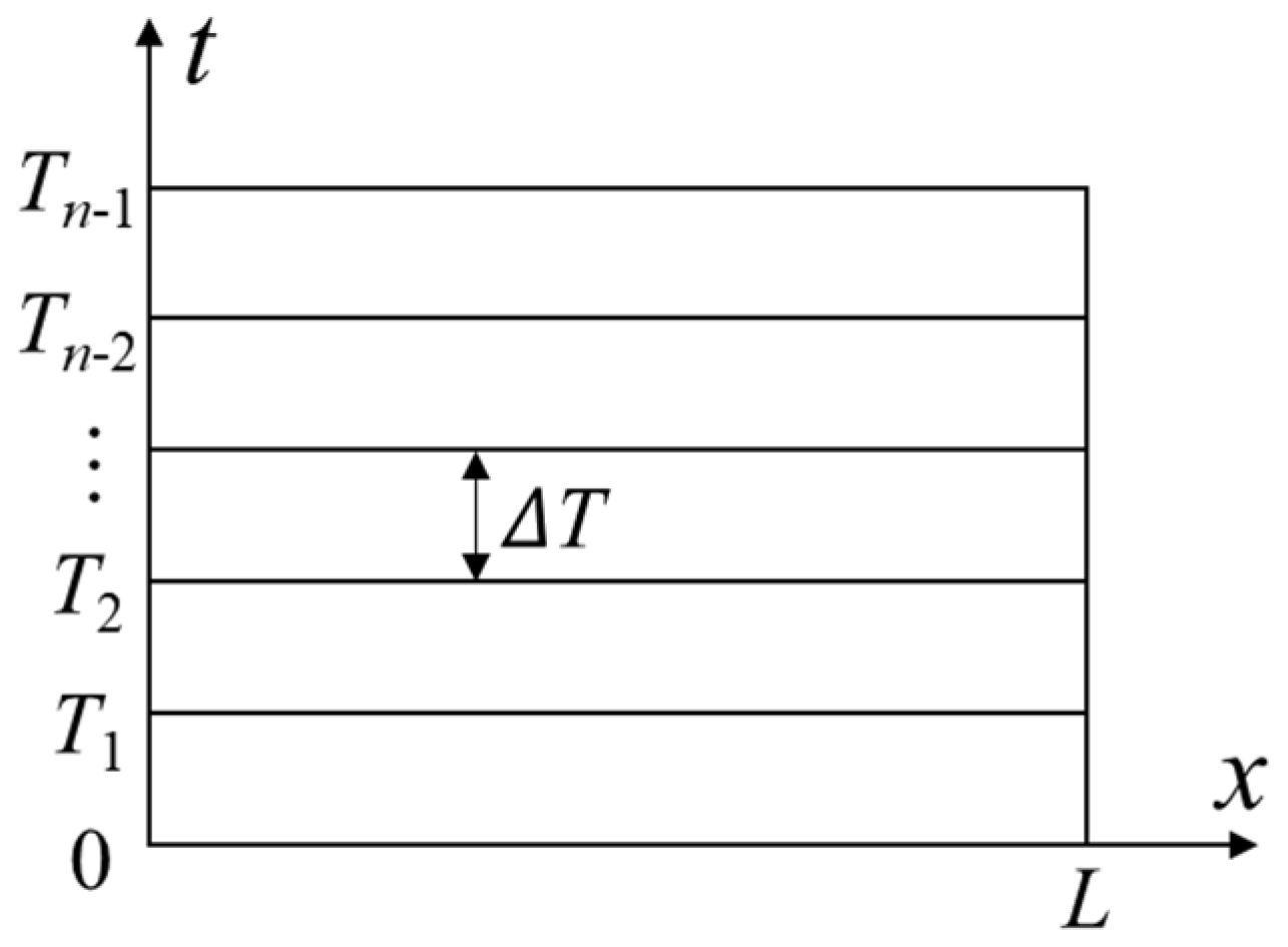
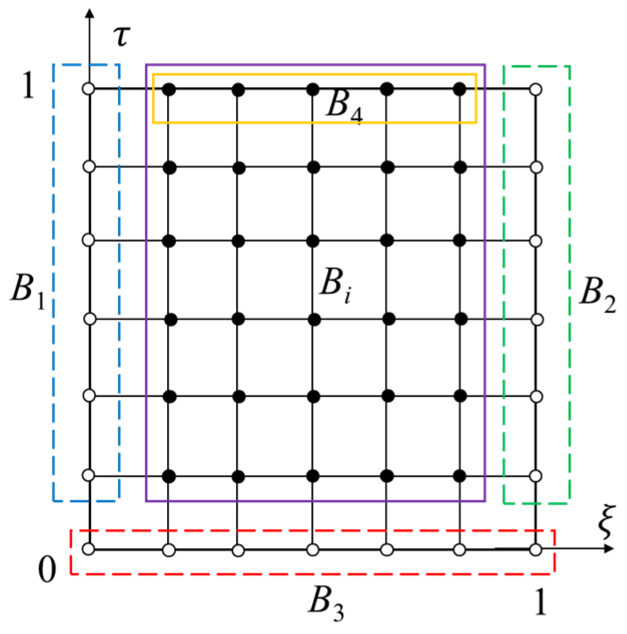
3.2. Space–Time Discretization and Numerical Scheme of DC Dynamic Analysis

For the above one-dimensional transient problem, a two-dimensional DC grid is needed for discretization. The orthogonal rectangular grids shown in Figure 1 are selected as the space–time discretization scheme, and the Equation (4) is discretized as the following form

$$\frac{EI}{L^4}{\displaystyle \sum _{k=1}^N{c}_{ik}^{({\xi }^4)}{y}_k}+\frac{\rho }{T^2}{\displaystyle \sum _{k=1}^N{c}_{ik}^{({\tau }^2)}{y}_k}-\frac{\rho \zeta }{T^2{L}^2}{\displaystyle \sum _{k=1}^N{c}_{ik}^{({\xi }^2{\tau }^2)}{y}_k}=F\left(L{\xi }_i,T{\tau }_i\right)$$

(9)

where $c_{ik}^{({\xi }^4)}$ and $c_{ik}^{({\tau }^2)}$ are the DC weight coefficients of the fourth order partial derivatives of $\xi$ and the second order partial derivatives of $\tau$, $c_{ik}^{({\xi }^2{\tau }^2)}$ is the fourth order mixed partial derivatives of $\xi$ and $\tau$, and N is the total number of discrete nodes.

If only one spatio–temporal grid is substituted into the calculation of the whole-time length T, in order to achieve the ideal accuracy, a considerable number of nodes need to be used, which will cause the matrix dimension to be too large and ill-conditioned. Therefore, in order to achieve long-term dynamic analysis, the whole space–time domain can be equally divided into (n−1) small space–time segments by referring to the progressive integration method. The length of each time step is $\Delta T$, and the equipartition process is shown in Figure 2.

For each time step $\Delta T$, its spatial–temporal discrete form is shown in Figure 3. Its initial time connects to the end of the previous time step. The initial displacement and initial velocity correspond to the displacement and velocity at the end of the previous time step. For convenience, group the nodes in the grid. Let the nodes at the initial time $\tau =0$ form B₃, the nodes satisfying $\xi =0$ and $\tau \ne 0$ form B₁, the nodes satisfying $\xi =1$ and $\tau \ne 0$ form B₂, all the remaining nodes form B_i, and the nodes satisfying $\tau =1$ in B_i form B₄. In particular, the case where any two combination symbols correspond to a combination of the underlying markers represents the union of the two node groups, such as B₁₂ being a combination of B₁ and B₂.

The gradual calculation method needs to extract the initial conditions (displacement and velocity) of each time step. At the same time, in order to substitute the boundary conditions, the discrete control Equation (9) needs to be reconstructed. Each partial derivative term in Equation (9) is decomposed as follows:

$$\begin{array}{ll}\hfill {\displaystyle \sum _{k=1}^N{c}_{ik}^{({\xi }^4)}{y}_k}& ={\displaystyle \sum _{k=B_{12}}{\displaystyle \sum _{j=B_N}{c}_{ik}^{({\xi }^2)}{c}_{kj}^{({\xi }^2)}{y}_j}}+{\displaystyle \sum _{k=B_{3i}}{\displaystyle \sum _{j=B_N}{c}_{ik}^{({\xi }^2)}{c}_{kj}^{({\xi }^2)}{y}_j}}\\ & =L^2{{\displaystyle \sum _{k=B_{12}}{c}_{ik}^{({\xi }^2)}\frac{{\partial }^{2}y}{\partial {\xi }^2}|}}_k+{\displaystyle \sum _{k=B_{3i}}{\displaystyle \sum _{j=B_N}{\displaystyle \sum _{l=B_{12}}{c}_{ik}^{({\xi }^2)}{c}_{kj}^{(\xi )}{c}_{jl}^{(\xi )}{y}_l}}}+{\displaystyle \sum _{k=B_{3i}}{\displaystyle \sum _{j=B_N}{\displaystyle \sum _{l=B_3}{c}_{ik}^{({\xi }^2)}{c}_{kj}^{(\xi )}{c}_{jl}^{(\xi )}{y}_l}}}\\ & +{\displaystyle \sum _{k=B_{3i}}{\displaystyle \sum _{j=B_N}{\displaystyle \sum _{l=B_i}{c}_{ik}^{({\xi }^2)}{c}_{kj}^{(\xi )}{c}_{jl}^{(\xi )}{y}_l}}}\end{array}$$

(10)

$$\begin{array}{ll}\hfill {\displaystyle \sum _{k=1}^N{c}_{ik}^{({\tau }^2)}{y}_k}& ={\displaystyle \sum _{k=B_3}{\displaystyle \sum _{j=B_N}{c}_{ik}^{(\tau )}{c}_{kj}^{(\tau )}{y}_j}}+{\displaystyle \sum _{k=B_{12i}}{\displaystyle \sum _{j=B_N}{c}_{ik}^{(\tau )}{c}_{kj}^{(\tau )}{y}_j}}\\ & =\Delta T{{\displaystyle \sum _{k=B_3}{c}_{ik}^{(\tau )}\frac{\partial y}{\partial \tau }|}}_k+{\displaystyle \sum _{k=B_{12i}}{\displaystyle \sum _{j=B_{12}}{c}_{ik}^{(\tau )}{c}_{kj}^{(\tau )}{y}_j}}+{\displaystyle \sum _{k=B_{12i}}{\displaystyle \sum _{j=B_3}{c}_{ik}^{(\tau )}{c}_{kj}^{(\tau )}{y}_j}}+{\displaystyle \sum _{k=B_{12i}}{\displaystyle \sum _{j=B_i}{c}_{ik}^{(\tau )}{c}_{kj}^{(\tau )}{y}_j}}\end{array}$$

(11)

$$\begin{array}{ll}{\displaystyle \sum _{k=1}^N{c}_{ik}^{({\xi }^2{\tau }^2)}{y}_k}& ={\displaystyle \sum _{k=B_N}{\displaystyle \sum _{j=B_3}{\displaystyle \sum _{l=B_N}{c}_{ik}^{({\xi }^2)}{c}_{kj}^{(\tau )}{c}_{jl}^{(\tau )}{y}_l}}}+{\displaystyle \sum _{k=B_N}{\displaystyle \sum _{j=B_{12i}}{\displaystyle \sum _{l=B_N}{c}_{ik}^{({\xi }^2)}{c}_{kj}^{(\tau )}{c}_{jl}^{(\tau )}{y}_l}}}\\ & =\Delta T{\displaystyle \sum _{k=B_N}{{\displaystyle \sum _{j=B_3}{c}_{ik}^{({\xi }^2)}{c}_{kj}^{(\tau )}\frac{\partial y}{\partial \tau }|}}_j}+{\displaystyle \sum _{k=B_N}{\displaystyle \sum _{j=B_{12i}}{\displaystyle \sum _{l=B_{12}}{c}_{ik}^{({\xi }^2)}{c}_{kj}^{(\tau )}{c}_{jl}^{(\tau )}{y}_l}}}\\ & +{\displaystyle \sum _{k=B_N}{\displaystyle \sum _{j=B_{12i}}{\displaystyle \sum _{l=B_3}{c}_{ik}^{({\xi }^2)}{c}_{kj}^{(\tau )}{c}_{jl}^{(\tau )}{y}_l}}}+{\displaystyle \sum _{k=B_N}{\displaystyle \sum _{j=B_{12i}}{\displaystyle \sum _{l=B_i}{c}_{ik}^{({\xi }^2)}{c}_{kj}^{(\tau )}{c}_{jl}^{(\tau )}{y}_l}}}\end{array}$$

(12)

Substituting the boundary conditions with simple support at both ends, that is, the displacement y and the first derivative of y of node group B₃ is zero. Substitute the Equations (11)–(13) into the Equation (9), and get

$$\begin{array}{l}(\frac{EI}{L^4}{\displaystyle \sum _{k=B_{3i}}{\displaystyle \sum _{j=B_N}{\displaystyle \sum _{l=B_i}{c}_{ik}^{({\xi }^2)}{c}_{kj}^{(\xi )}{c}_{jl}^{(\xi )}}}}+\frac{\rho }{\Delta T^2}{\displaystyle \sum _{k=B_{12i}}{\displaystyle \sum _{l=B_i}{c}_{ik}^{(\tau )}{c}_{kl}^{(\tau )}}}-\frac{\rho \zeta }{\Delta T^2{L}^2}{\displaystyle \sum _{k=B_N}{\displaystyle \sum _{j=B_{12i}}{\displaystyle \sum _{l=B_i}{c}_{ik}^{({\xi }^2)}{c}_{kj}^{(\tau )}{c}_{jl}^{(\tau )}}}})y_l=F_i+\\ (\frac{\rho \zeta }{\Delta T^2{L}^2}{\displaystyle \sum _{k=B_N}{\displaystyle \sum _{j=B_{12i}}{\displaystyle \sum _{l=B_3}{c}_{ik}^{({\xi }^2)}{c}_{kj}^{(\tau )}{c}_{jl}^{(\tau )}}}}-\frac{EI}{L^4}{\displaystyle \sum _{k=B_{3i}}{\displaystyle \sum _{j=B_N}{\displaystyle \sum _{l=B_3}{c}_{ik}^{({\xi }^2)}{c}_{kj}^{(\xi )}{c}_{jl}^{(\xi )}}}}-\frac{\rho }{\Delta T^2}{\displaystyle \sum _{k=B_{12i}}{\displaystyle \sum _{l=B_3}{c}_{ik}^{(\tau )}{c}_{kl}^{(\tau )}}})y_l\\ +\left(\frac{\rho \zeta }{\Delta T{L}^2}{\displaystyle \sum _{k=B_N}{\displaystyle \sum _{l=B_3}{c}_{ik}^{({\xi }^2)}{c}_{kl}^{(\tau )}}}-\frac{\rho }{\Delta T}{\displaystyle \sum _{l=B_3}{c}_{il}^{(\tau )}}\right){\frac{\partial y}{\partial \tau }|}_l\end{array}$$

(13)

where $i=B_i$

Equation (13) can be written as a matrix form

$$\tilde{\mathit{K}}{Y}_{B_i}=\tilde{\mathit{F}}$$

(14)

where

$$\begin{array}{ll}\hfill \tilde{\mathit{K}}& =\frac{EI}{L^4}{W}_{B_i,B_{3i}}^{({\xi }^2)}{W}_{B_{3i},B_N}^{(\xi )}{W}_{B_N,B_i}^{({\xi }^2)}+\frac{\rho }{\Delta T^2}{W}_{B_i,B_{12i}}^{(\tau )}{W}_{B_{12i},B_i}^{(\tau )}\\ & -\frac{\rho \zeta }{\Delta T^2{L}^2}{W}_{B_i,B_N}^{({\xi }^2)}{W}_{B_i,B_{12i}}^{(\tau )}{W}_{B_{12i},B_i}^{(\tau )}\end{array}$$

(15)

$$\begin{array}{ll}\hfill \tilde{\mathit{F}}& =F+(\frac{\rho \zeta }{\Delta T^2{L}^2}{W}_{B_i,B_N}^{({\xi }^2)}{W}_{B_N,B_{12i}}^{(\tau )}{W}_{B_{12i},B_3}^{(\tau )}\\ & -\frac{EI}{L^4}{W}_{B_i,B_{3i}}^{({\xi }^2)}{W}_{B_{3i},B_N}^{(\xi )}{W}_{B_N,B_3}^{(\xi )}-\frac{\rho }{\Delta T^2}{W}_{B_i,B_{12i}}^{(\tau )}{W}_{B_{12i},B_3}^{(\tau )})y_0\\ & +\left(\frac{\rho \zeta }{\Delta T{L}^2}{W}_{B_i,B_N}^{({\xi }^2)}{W}_{B_N,B_3}^{(\tau )}-\frac{\rho }{\Delta T}{W}_{B_i,B_3}^{(\tau )}\right){\dot{\mathit{y}}}_0\end{array}$$

(16)

According to Equation (14),

$$Y_{B_i}={\tilde{\mathit{K}}}^{-1}\tilde{\mathit{F}}$$

(17)

Based on the DC principle, the unknown velocity vector ${\dot{\mathit{Y}}}_{B_i}$ in a time step is the first derivative of displacement to time, namely

$${\dot{\mathit{Y}}}_{B_i}=\frac{1}{\Delta T}{W}_{B_i,B_i}^{(\tau )}{\tilde{\mathit{K}}}^{-1}\tilde{\mathit{F}}+\frac{1}{\Delta T}{W}_{B_i,B_3}^{(\tau )}{y}_0$$

(18)

According to Equations (15) and (16), the displacement and velocity vectors at the end of the step at the internal point except the boundary at both ends are

$$Y_{B_4}=\Gamma {\tilde{\mathit{K}}}^{-1}\tilde{\mathit{F}}$$

(19)

$${\dot{\mathit{Y}}}_{B_4}=\frac{\Gamma }{\Delta T}\left(W_{B_i,B_i}^{(\tau )}{\tilde{\mathit{K}}}^{-1}\tilde{\mathit{F}}+W_{B_i,B_3}^{(\tau )}{y}_0\right)$$

(20)

where $\Gamma$ represents the transformation matrix used to extract the node displacement at the end of all unknown node displacements. The matrix has (m − 2) rows, corresponding to node group B₄ which represents nodes at the end of the time step. The matrix has (N − 2n − m + 2) columns, corresponding to node group B_i which represents the nodes to be solved. Suppose that B_i denotes the node number from 1 to (N − 2n − m + 2) and B₄ denotes the node number from 1 to (m − 2), then $\Gamma$ can be expressed as

$$\Gamma ={\left[\begin{array}{ccccccc}1& 0& \cdots & 0& 0& 0& 0\\ 0& 1& \cdots & 0& 0& 0& 0\\ ⋮& ⋮& \ddots & 0& ⋮& ⋮& ⋮\\ 0& 0& 0& 1& 0& 0& 0\end{array}\right]}_{(m-2)\times (N-2n-m+2)}$$

Equation (16) is abbreviated as the following form

$$\tilde{\mathit{F}}=F+W_0{y}_0+W_{00}{\dot{\mathit{y}}}_0$$

(21)

where

$$W_0=\frac{\rho \zeta }{\Delta T^2{L}^2}{W}_{B_i,B_N}^{({\xi }^2)}{W}_{B_N,B_{12i}}^{(\tau )}{W}_{B_{12i},B_3}^{(\tau )}-\frac{EI}{L^4}{W}_{B_i,B_{3i}}^{({\xi }^2)}{W}_{B_{3i},B_N}^{(\xi )}{W}_{B_N,B_3}^{(\xi )}-\frac{\rho }{\Delta T^2}{W}_{B_i,B_{12i}}^{(\tau )}{W}_{B_{12i},B_3}^{(\tau )}$$

(22)

$$W_{00}=\frac{\rho \zeta }{\Delta T{L}^2}{W}_{B_i,B_N}^{({\xi }^2)}{W}_{B_N,B_3}^{(\tau )}-\frac{\rho }{\Delta T}{W}_{B_i,B_3}^{(\tau )}$$

(23)

Substituting Equations (22) and (23) into Equation (19), we can obtain

$$Y_{B_4}=\Gamma {\tilde{K}}^{-1}\left(F+W_0{y}_0+W_{00}{\dot{\mathit{y}}}_0\right)$$

(24)

$${\dot{\mathit{Y}}}_{B_4}=\frac{\Gamma }{\Delta T}(W_{B_i,B_i}^{(\tau )}{\tilde{\mathit{K}}}^{-1}F+\left(W_{B_i,B_i}^{(\tau )}{\tilde{K}}^{-1}{W}_0+W_{B_i,B_3}^{(\tau )}\right)y_0+W_{B_i,B_i}^{(\tau )}{\tilde{\mathit{K}}}^{-1}{W}_{00}{\dot{\mathit{y}}}_0)$$

(25)

Equations (24) and (25) can be written as the following recursive format

$$\left\{\begin{array}{c}{Y}_{B_4}\\ {\dot{Y}}_{B_4}\end{array}\right\}=Q\left\{\begin{array}{c}{y}_0\\ {\dot{y}}_0\end{array}\right\}+J_1$$

(26)

where Q is a transfer matrix, and

$$Q=\left[\begin{array}{cc}\Gamma {\tilde{K}}^{-1}{W}_0& \Gamma {\tilde{\mathit{K}}}^{-1}{W}_{00}\\ \frac{\Gamma }{\Delta T}\left(W_{B_i,B_i}^{(\tau )}{\tilde{K}}^{-1}{W}_0+W_{B_i,B_3}^{(\tau )}\right)& \frac{\Gamma }{\Delta T}{W}_{B_i,B_i}^{(\tau )}{\tilde{\mathit{K}}}^{-1}{W}_{00}\end{array}\right]$$

$$J_1=\left\{\begin{array}{c}\Gamma {\tilde{\mathit{K}}}^{-1}F\\ \frac{\Gamma }{\Delta T}{W}_{B_i,B_i}^{(\tau )}{\tilde{\mathit{K}}}^{-1}F\end{array}\right\}$$

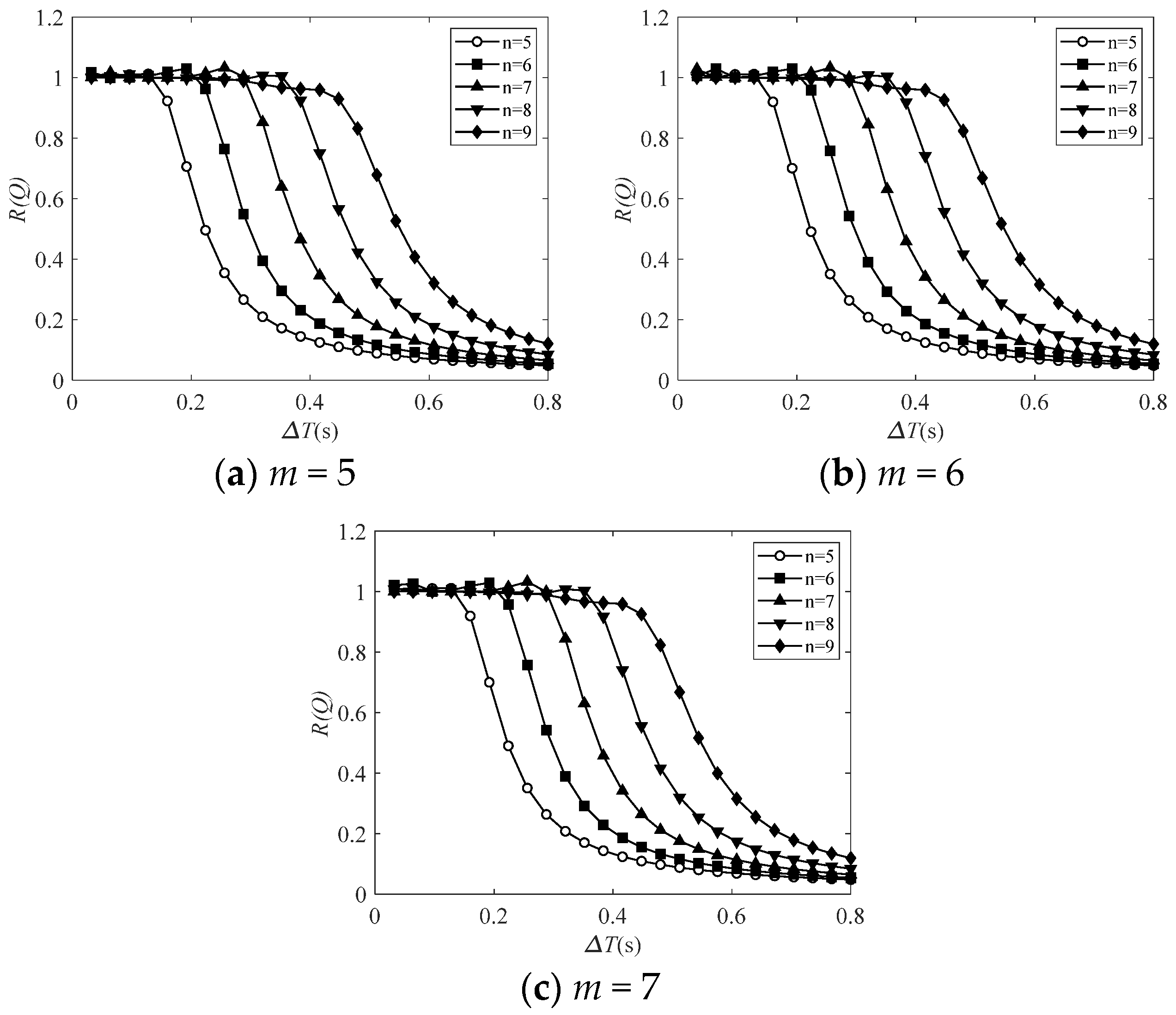
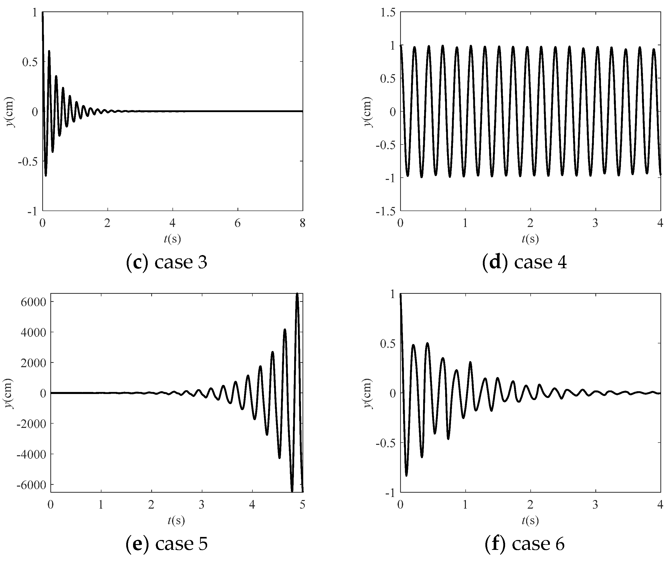
3.3. Stability Analysis of Transfer Matrix Q

The stability of recurrence process is analyzed based on the spectral radius R(Q) of transfer matrix in Equation (26). According to the construction of Q, if the attribute parameters of the beam are determined, the transfer matrix is only related to the DC weight coefficient and the time step $\Delta T$. Orthogonal grids are selected as discrete schemes, so that the number of boundary nodes in $\xi$ and $\tau$ directions is m and n respectively. When the basis function scheme is determined, the DC weight coefficients are determined by m and n.

The specific property parameters of the beam are as follow: rigidity EI = 4.7726 $\times$ 10⁷ N/m; distributed mass $\rho$ = 420 kg/m; length L = 0.01 m; and shear coefficient $\zeta =30/{\pi }^2$. Firstly, by controlling the time step $\Delta T$ = 0.25 s, the relationship between R(Q) and orthogonal grids of m and n under different conditions is explored, where the uniform distribution of nodes and the nodes of CGL distribution form are considered.

Figure 4 shows the curves of R(Q) versus n for m = 3, 4, 5, respectively. Each case includes two distributions for comparison.

It can be seen from Figure 4 that R(Q) in the case of CGL distribution increases gradually to 1 with the increase of n, and then remains stable around 1. In the case of uniform distribution, R(Q) will have a mutation at the position of n = 6 or 7, and the trends expect above mutation are roughly the same as for the CGL distribution. It can be discovered that the spectral radius under the two distributions is generally less than or equal to 1, but the range of spectral radius close to 1 under the CGL distribution is wider.

Then the effect of time step $\Delta T$ on spectral radius R(Q) of transfer matrix is studied. As shown in Figure 5, the relationship curves between the spectral radius and the time step length calculated under different grids of m and n are given. In general, R(Q) first maintains a process near 1 with the increase of $\Delta T$, then begins to decline rapidly at a certain point, and, finally, gradually converges to a smaller value. The position of the sudden drop varies with the number of nodes in the time domain, that is, when m is the same, the larger n, the later the drop, and the wider the range of R(Q) close to 1. In addition, by comparing these three figures, it can be found that increasing the number of nodes m in the spatial direction alone has little effect on the value of R(Q). The spectral radius of the transfer matrix Q is close to or less than 1 on orthogonal grids, where the main difference is the range width of R(Q) near 1.

In order to study the time-history displacement of the transmission process under different values of R(Q), several specific conditions are selected according to the grid form and time step length to do the stability verification analysis. The specific conditions are shown in

Table 1. R(Q) under different mesh forms and time steps.

	m = 5, n = 5			m = 5, n = 7
	Case 1	Case 2	Case 3	Case 4	Case 5	Case 6
distribution form	CGL	CGL	CGL	CGL	equally spaced	CGL
$\Delta T$(s)	0.064	0.16	0.2	0.16	0.25	0.35
R(Q)	1.0015	0.9229	0.6477	0.9984	1.5524	0.6521

.

Let the initial displacement and initial velocity of the beam be respectively

$${(y)}_{\tau =0}=\sin (\pi \xi )$$

(27)

$${\left(\partial y/\partial \tau \right)}_{\tau =0}=0$$

(28)

The time-history displacement patterns of free vibration with Equation (21) as initial conditions in 6 cases in Table 1 are studied, and the curves are shown in Figure 6.

First, Figure 6a–c are observed, which is the time history displacement of the CGL distributed orthogonal grid with m = n = 5 at different time steps. Figure 6a shows a normal harmonic free vibration with the value of R(Q) close to 1. When the step increases, the spectral radius decreases, and the time-history displacements of cases 2 and 3 show the attenuation form, and the smaller the R(Q) value is, the faster the attenuation speed is. Then Figure 6d–f are observed, where the orthogonal grid with m = 5, n = 7 is given, including two kinds of distribution form of nodes at different time steps. Figure 6d also shows a harmonic free vibration the value of R(Q) close to 1. The time-history displacement amplitude in Figure 6e increases with time and reaches three orders of magnitude of 10 at 4 s, showing a state of instability. Corresponding to the situation that the spectral radius value of the uniformly distributed orthogonal grid in Figure 4c is greater than 1 when m = 5 and n = 7. Time history displacement in Figure 6f attenuates with time, corresponding to the case 6 where R(Q) far less than 1. The rules of time history displacement corresponding to different spectral radius values in orthogonal grids can be found by combining above six figures:

(1)

When the spectral radius R(Q) is close to 1, the time-history displacement shows a stable form. To a certain extent, when it is less than 1, the time-history displacement of free vibration will gradually decay, and the decay rate is negatively correlated with R(Q).

(2)

When the spectral radius R(Q) is greater than 1 to a certain extent, it will lead to the accumulation and amplification of errors, and eventually lead to instability.

Based on the above rules, in order to make the time history displacement tend to be stable over time, we need to make R(Q) as close to 1 as much as possible when using orthogonal grids as space–time discretization schemes, and, according to Figure 5, increasing the number of nodes in the time domain direction of the grid is a more effective method to expand the stability range.

3.4. Forced Vibration Analysis of Beams

In the previous section, the stability of the DC method in analyzing dynamic problems is analyzed. Next, the displacement response of a Timoshenko shear beam under dynamic load F(x, t) is presented in this paper. The expression of dynamic load is

$$F(x,t)=Q\sin \frac{\pi x}{L}\sin st$$

(29)

where Q is the peak load and s is the time-domain variation frequency of load.

Considering that the boundary condition is simply supported at both ends, and the initial condition is that the displacement and velocity at t = 0 are zero. The displacement analytical solution of forced vibration of the Timoshenko shear beam under load F(x, t) is

$$y(x,t)=\frac{Q}{\rho \left[1+\zeta {(\pi /L)}^2\right]}\sin \left(\frac{\pi x}{L}\right)\frac{\sin st-(s/\omega )\sin \omega t}{{\omega }^2-s^2}$$

(30)

where $\omega$ is the foundation natural frequency of the beam, and the expression is

$$\omega ={\pi }^2\sqrt{\frac{EI}{\rho L^4\left[1+\zeta {(\pi /L)}^2\right]}}$$

(31)

The attribute parameters of the beam remain unchanged, and the relevant parameters of the load are: the peak load Q = 10⁷ N; $s=2\pi /0.28335$; and Time step $\Delta T$ = 0.25 s. The values of the total time T are taken at 2.5 s and 5 s respectively. According to the value of $\Delta T$, the total time T is divided into 10 and 20 time steps. The orthogonal grid of CGL distribution with m = 7, n = 9 is used for calculation, and the DC solution is compared with the analytical solution obtained by Equation (30). Figure 7 and Figure 8 give the displacement of DC solutions and the analytical solutions of the nodes on the beam under the whole-time history, in which the curves of the DC solution and the analytical solution are always perfectly consistent, with no phenomenon of detachment over time.

Table 2. Comparison of DC solution and analytic solution for time-history displacement of Timoshenko beam.

t	x/L = 0.067			x/L = 0.25			x/L = 0.5
	DC Solution	Exact	Error(%)	DC Solution	Exact	Error(%)	DC Solution	Exact	Error(%)
0.5	−17.8585	−17.8586	−0.0006	−60.4521	−60.4507	0.0023	−85.4954	−85.4902	0.0061
1.0	4.4188	4.4173	0.0340	14.9579	14.9522	0.0381	21.1544	21.1457	0.0411
1.5	11.9420	11.9414	0.0050	40.4245	40.4211	0.0084	57.1711	57.1641	0.0122
2.0	−4.0400	−4.0345	0.1363	−13.6756	−13.6567	0.1384	−19.3410	−19.3135	0.1424
2.5	−4.3708	−4.3747	−0.0891	−14.7953	−14.8083	−0.0878	−20.9244	−20.9421	−0.0845
3.0	−2.2223	−2.2274	−0.2290	−7.5225	−7.5398	−0.2294	−10.6388	−10.6629	−0.2260
3.5	0.4370	0.4372	−0.0457	1.4553	1.4799	−1.6623	2.0940	2.0929	0.0526
4.0	10.8579	10.8553	0.0240	36.7545	36.7448	0.0264	51.9807	51.9650	0.0302
4.5	−2.3860	−2.3960	−0.4174	−8.0769	−8.1104	−0.4130	−11.4229	−11.4698	−0.4089
5.0	−16.4010	−16.3886	0.0757	−55.5183	−55.4748	0.0784	−78.5177	−78.4532	0.0822

shows the detailed data comparison between the displacement DC solution and the analytical solution of the beam node at each moment. It can be seen that the errors between DC solutions and analytical solutions are almost kept within one percent, more than half of the data errors remain within one thousand, and there is no sign of error accumulation and amplification.

By comparing the data in Figure 7 and Figure 8 and Table 2, it is found that highly accurate results can be obtained by applying the DCM for calculating the forced vibration of the beam. Then, this paper will continue to use the space–time DCM to analyze the influence factors of time-history displacement form of beam under dynamic load.

The displacement form of the beam under forced vibration is mainly determined by the relative relationship between the natural vibration frequency $\omega$ of the beam and the change frequency s of the load in time. According to Equation (31), the fundamental natural frequency $\omega$ of the beam is determined by the bending stiffness EI, distributed mass $\rho$, beam length L and shear coefficient $\zeta$. Keep the other three factors unchanged to study the effect of EI on time history displacement, as shown in

Table 3. Bending stiffness and natural vibration frequency of foundation under different conditions (s = 22.1746).

	Case 1	Case 2	Case 3	Case 4	Case 5	Case 6
EI	7.772 $\times$ 104	4.772 $\times$ 105	4.772 $\times$ 106	2.772 $\times$ 107	4.772 $\times$ 108	4.772 $\times$ 109
$\omega$	1.1776	2.9180	9.2274	22.2406	92.2743	291.7971

. Figure 9 shows the time history displacements in six cases in Table 3. As an influencing factor, bending stiffness EI affects the value of foundation natural frequency $\omega$, and the relative relationship between $\omega$ and load variation frequency s determines the displacement time-history shape of these six figures. When the value of EI is small and $\omega$ is small relative to s, as in case 1 and 2, the main trend of displacement is determined by the natural frequency of the foundation, and external load F(x, t) has only a small effect on the time-history displacement, which is reflected in small fluctuations in Figure 9a,b. When EI increases, the effect of small fluctuations caused by F(x, t) becomes obvious. When EI continues to increase so that $\omega$ reaches about 0.4 times of s, as in case 3, the effect of load frequency s on time-history displacement is very obvious, completely disturbing the dominant trend of natural frequency on time-history displacement. When natural frequency $\omega$ is close to load frequency s, as shown in case 4 of Figure 9d, resonance occurs, and the displacement amplitude increases with time. When the increase of EI makes $\omega$ much larger than s, as shown in cases 5 and 6 of Figure 9e,f, the trend of time-history displacement is mainly determined by the load frequency. In addition, the bending stiffness not only affects the natural frequency of the structure, but also has a dominant influence on the maximum displacement of the structure. In structural mechanics, the stiffness is defined as the force required for the unit displacement of the structure. Therefore, when the bending stiffness increases gradually, the maximum displacement in the time-history displacement will also decrease, which is consistent with the data in the Figure 9.

The analytical solution curves are also given as a comparison. It can be found that the two are in good agreement, which indicates that the dynamic analysis of beam structure by DCM is reasonable and accurate.

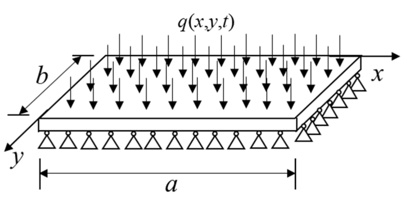
4. Space–Time Dynamic Analysis of Forced Vibration of Thin Plate

4.1. Dynamic Equation and Initial and Boundary Conditions

As shown in Figure 10, the dynamic differential equations of thin plates with length and width of a and b under uniform dynamic load q are

$$\frac{{\partial }^{4}w}{\partial x^4}+2\frac{{\partial }^{4}w}{\partial x^2\partial y^2}+\frac{{\partial }^{4}w}{\partial y^4}+\frac{\rho h}{D}\frac{{\partial }^{2}w}{\partial t^2}=\frac{q(x,y,t)}{D}$$

(32)

where w is the transverse displacement of the plate, $\rho$ is the density, h is the thickness of the plate, E is the elastic modulus, v is the Poisson’ s ratio, and D is the bending stiffness of the plate, whose expression is

$$D=\frac{E{h}^3}{12(1-v^2)}$$

Consider simply supported boundary conditions

$${(w)}_{x=0,a}=0$$

(33)

$${\left({\partial }^{2}w/\partial x^2\right)}_{x=0,a}=0$$

(34)

The initial value condition is

$${(w)}_{\tau =0}={(\dot{w})}_{\tau =0}=0$$

(35)

4.2. Discrete Form of Three-Dimension DC Grid

Since the thin plate is a two-dimensional model in space, it becomes a three-dimensional problem to increase the time dimension on this basis. Therefore, in order to use the DC method for spatial and temporal analysis, three dimensional grids are needed. As shown in Figure 11, suppose the number of nodes in the x-direction and y-direction are m and n respectively, a two-dimensional orthogonal grid of m × n is formed at t = 0. Copy the mesh up k times in turn to form a 3D orthogonal mesh of m × n × k.

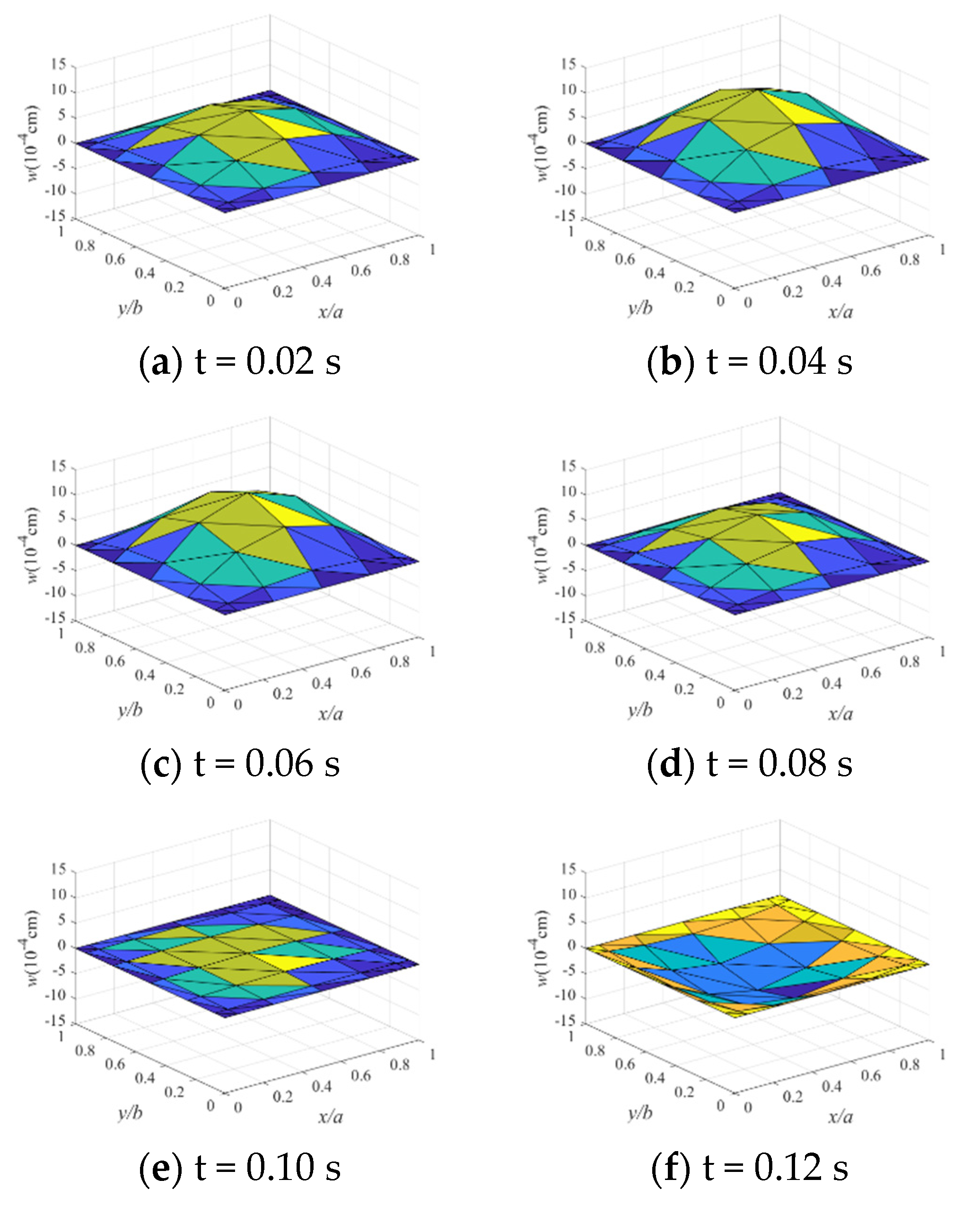
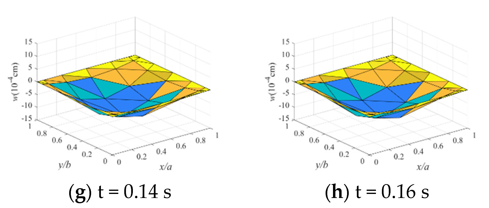
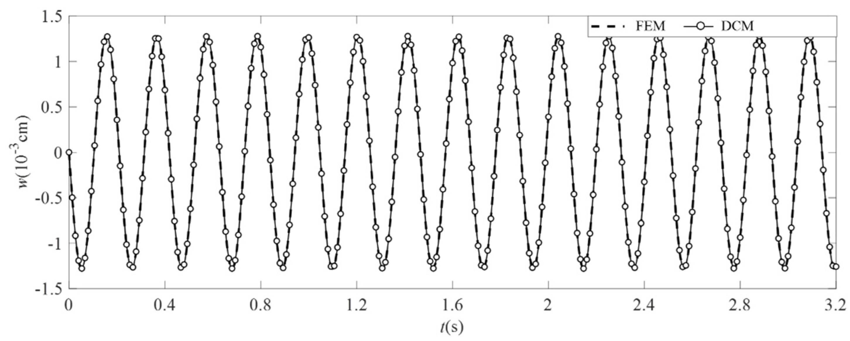
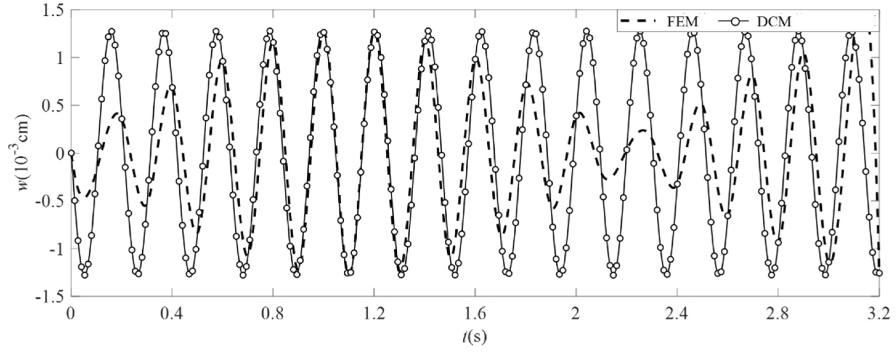
4.3. Analysis Results and Comparison

For the thin plate in Figure 10, let its length a and width b be 0.8 m, thickness h = 0.01 m, elastic modulus E = 1.5 × 10¹¹ N/m², Poisson ‘s ratio v = 0.2, density $\rho$ = 8000 kg/m³, the value of initial velocity and initial displacement be 0, and the time-dependent uniform load q(x,y,t) = 10,000sin (30t) N/m².

Firstly, all displacements in a time step are calculated by using orthogonal grids of 5 × 5 × 9 and 7 × 7 × 9, respectively, where the CGL orthogonal grids are 5 × 5 and 7 × 7 on the x-y plane and 9 uniformly distributed spatial nodes in the t direction. Let the time step length be 0.16 s, the displacement obtained by DCM at each time step is compared with the analytical solution and the relevant reference solution. The comparison results are shown in

Table 4. The displacement at 8 time points of the center point of the four simply supported thin plate under the action of dynamic load q.

t(s)	Exact [29] (10−4 cm)	Reference [30] (10−4 cm)	Error 1 (%)	5 × 5 × 9 DC (10−4 cm)	Error 2 (%)	7 × 7 × 9 DC (10−4 cm)	Error 3 (%)
0.02	7.22	7.4243	2.83	7.1684	0.7184	7.2166	0.0471
0.04	11.92	12.1476	1.91	11.8333	0.7273	11.9129	0.0596
0.06	12.45	12.6330	1.47	12.3641	0.6900	12.4472	0.0225
0.08	8.637	8.7165	0.92	8.5758	0.7086	8.6335	0.0405
0.10	1.804	1.7890	−0.83	1.7917	0.6818	1.8037	0.0166
0.12	−5.658	−5.5115	−2.59	−5.6183	−0.7017	−5.6561	−0.0336
0.14	−11.14	−11.4976	3.21	−11.0657	−0.6670	−11.1401	−0.0009
0.16	−12.74	−12.9477	1.63	−12.6471	−0.7292	−12.7321	−0.0620

. Figure 12 shows the global displacement of the 7 × 7 × 9 orthogonal grid corresponding to the eight moments in Table 4 as a reference.

According to the data in Table 4, the error between the finite element solution and the analytical solution in the literature is roughly maintained at 1–3%. The grid of 21 × 21 is used in space, and the stepwise method is used in time domain. The minimum step of segmentation is 0.01 s in FEM. In this paper, the error between the results obtained by DCM with the orthogonal grid of 5 × 5 × 9 and the analytical solution is less than one percent and is uniformly distributed over time. When the orthogonal grid of 7 × 7 × 9 is used, the error between the displacement solution and the analytical solution is kept within one thousandth.

Next, the total time T of the above load action is set to be 3.2 s, and the orthogonal grid of 5 × 5 × 9 is used for calculation. The length of each time step is set to 0.16 s, so a total of 20 time steps are required. As a reference, the finite element software Abaqus is used to calculate. Three-dimensional shell elements are selected, the number of elements is 20 × 20, and the time steps are 0.01 s, 0.05 s, and 0.1 s, respectively. Still taking the center node of the plate as the reference point, the time-history displacement curves of the center point of the plate calculated by two methods are shown in Figure 13, Figure 14 and Figure 15.

It can be seen from Figure 13 and Figure 14 that the calculation results of DC method with a 5 × 5 × 9 orthogonal grid based on 0.16 s time step are consistent with the calculation results of DCM with a 21 × 21 grid based on 0.01 s and 0.05 s time steps, indicating the correctness of the method used in this paper. In addition, it can be found from Figure 15 that when the time step of 0.1 s is adopted by FEM, the displacement no longer keeps sinusoidal variation, but is in a state of amplitude increasing first and then decreasing, which indicates that the calculation results of FEM with this time step are already in an unstable state, and the correct results cannot be obtained.

Table 5. Calculating time of FEM and DCM.

Numerical Method	FEM(20 × 20)			DCM
	ΔT = 0.1 s	ΔT = 0.05 s	ΔT = 0.01 s	(5 × 5 × 9)	(7 × 7 × 9)
cpu-time (s)	17	23	47	0.4394	0.8663

shows the computation time of FEM and DCM in this case. When the time step of FEM is 0.1 s, the computation time is 17 s, but the correct result is not obtained. When the time step decreases, the computation time increases. The calculation time of DCM under two orthogonal grids is less than 1 s, and extremely accurate results can be obtained. Based on the above comparison with FEM, the following conclusions can be obtained: when dealing with the dynamic response problem on the plate with long duration, DCM can obtain more accurate results with less computational time.

5. Conclusions

A spatio–temporal dynamic analysis method based on multi-dimensional differential quadrature principle is proposed, and one-dimensional and two-dimensional transient problems are analyzed, respectively. For one-dimensional transient problems, the vibration problem of the Timoshenko shear beam is taken as an example in this paper. Based on a two-dimensional orthogonal grid, the dynamic response equation is discretized in time and space. Due to the limited time step length of a space–time grid, considering the time consuming and the problem duration, this paper combines the space–time DC method with the step-by-step method to solve the long-time domain problem.

Combined with the step-by-step method, the original discrete control equation needs to be processed, and the initial displacement and velocity of each time step are extracted to facilitate the cyclic recursion of each time step. In order to study the stability of the recursive process, this paper constructs the transfer matrix of the control equation and studies the factors affecting the stability of the transfer process by combining the spectral radius of the matrix and the time-history displacement of the free vibration of the Timoshenko beam. When the number of nodes in the spatial direction of orthogonal grid is constant, increasing the nodes in the temporal direction is conducive to improving the stability of the transfer process. The longer the calculation steps, the worse the stability of the transfer process. For the forced vibration problem of the beam, when the appropriate grid is selected, the calculation results of the DC method are in good agreement with the analytical solution, and there is no error accumulation with the increase of time. In addition, the DCM is used to investigate the influence of the relative relationship between the natural frequency of the beam foundation and the frequency of the load on the time history displacement of the forced vibration of the beam. The results are consistent with the analytical solution.

For two-dimensional transient problems, space domain and time domain are three dimensions, this paper selects a three-dimensional orthogonal grid. Taking the forced vibration of a thin plate simply supported under the uniformly distributed load with periodic variation as an example, the appropriate grid is selected, and the calculation results are compared with the analytical solution and the finite element solution. It is found that when the DC method is used, the results can still be better than those of the finite element method with less space nodes and relatively large time step, and the calculation time is very small. These comprehensively reflect the accuracy and efficiency of the DCM in dealing with time domain problems.

References

1. Cloughr, W.; Penzien, J. Dynamics of Structures, 2nd ed.; Revised; Computers and Structures, Inc.: New York, NY, USA, 2003; pp. 156–219. [Google Scholar]
2. Chopra, A.K. Dynamics of Structures: Theory and Applications to Earthquake Engineerin, 3rd ed.; Tsinghua University Press: Beijing, China, 2009; pp. 815–836. [Google Scholar]
3. Houbolt, J.C. A recurrence matrix solution for the dynamic response of elastic aircraft. J. Aeronaut. Sci. 1950, 17, 540–550. [Google Scholar] [CrossRef]
4. Newmark, N.M. A method of computation for structural dynamics. J. Eng. Mech. Div. 1959, 85, 67–94. [Google Scholar] [CrossRef]
5. Wilson, E.L.; Farhoomand, I.; Bathe, K.J. Nonlinear dynamic analysis of complex structures. Earthq. Eng. Struct. Dyn. 1973, 1, 241–252. [Google Scholar] [CrossRef]
6. Bellman, R.; Casti, J. Differential quadrature and long-term integration. J. Math. Anal. Appl. 1971, 34, 235–238. [Google Scholar] [CrossRef] [Green Version]
7. Bellman, R.; Kashef, B.G.; Casti, J. Differential quadrature: A technique for the rapid solution of nonlinear partial differential equations. J. Comput. Phys. 1972, 10, 40–52. [Google Scholar] [CrossRef]
8. Bert, C.W.; Malik, M. Differential quadrature method in computational mechanics: A review. Appl. Mech. Rev. 1996, 49, 1–28. [Google Scholar] [CrossRef]
9. Xinwei, W. Differential quadrature in the analysis of structural components. Adv. Mech. 1995, 25, 232–240. (In Chinese) [Google Scholar]
10. Fung, T.C. Stability and accuracy of differential quadrature method in solving dynamic problems. Comput. Methods Appl. Eng. 2002, 191, 1311–1331. [Google Scholar] [CrossRef]
11. Fung, T. Solving initial problems by differential quadrature method, Part 1: First-order equations. Int. J. Numer. Methods Eng. 2001, 50, 1411–1427. [Google Scholar] [CrossRef]
12. Shu, C.; Yao, Q.; Yeo, K.S. Block-marching in time with DQ discretization: An efficient method for time-dependent problems. Comput. Methods Appl. Mech. Eng. 2002, 191, 4587–4597. [Google Scholar] [CrossRef]
13. Liu, J.; Wang, X. An assessment of the differential quadrature time integration scheme for nonlinear dynamic equations. J. Sound Vib. 2008, 314, 246–253. [Google Scholar] [CrossRef]
14. Tong, L.H.W. A time-stepping method of seismic response analysis for structures using differential quadrature rule. Chin. J. Theor. Appl. Mech. 2011, 43, 430–435. (In Chinese) [Google Scholar]
15. Hongjing, L.; Xu, L.; Tong, W. Two numerical schemes of differential quadrature analysis procedure for response of the earthquake-resistant structures. J. Basic Sci. Eng. 2011, 19, 758–766. (In Chinese) [Google Scholar]
16. Yuchen, M.; Hongjing, L.; Guangjun, S. Basic characteristics of differential quadrature method for dynamic response analysis of structures. J. Vib. Shock. 2020, 39, 214–221. (In Chinese) [Google Scholar]
17. Civan, F. Solving multivariable mathematical models by the quadrature and cubature method. Numer. Method Partial. Differ. Equ. 1994, 10, 545–567. [Google Scholar] [CrossRef]
18. Malik, M.; Civan, F. A comparative study of differential quadrature and cubature methods vis-à-vis some conventional techniques in context of convection-diffusion-reaction problems. Chem. Eng. Sci. 1995, 50, 531–547. [Google Scholar] [CrossRef]
19. Leiw, K.M.; Liu, F.L. Differential cubature method for Kirchhoff plates of arbitrary shape. Comput. Methods Appl. Mech. Eng. 1997, 145, 1–10. [Google Scholar] [CrossRef]
20. Liu, F.L.; Liew, K.M. Differential cubature method for static solutions of arbitrarily shaped thick plates. Int. J. Solids Struct. 1998, 35, 3655–3674. [Google Scholar] [CrossRef]
21. Wu, L.; Feng, W. Differential cubature method for buckling analysis of arbitrary quadrilateral thick plates. Struct. Eng. Mech. 2003, 16, 259–274. [Google Scholar] [CrossRef]
22. Pang, G.F.; Chen, W.; Sze, K.Y. Differential quadrature and cubature methods for steady-state space-fractional advection-diffusion equations. Comput. Modeling Eng. Sci. 2014, 97, 299–322. [Google Scholar]
23. Wu, L.; Li, J.; Li, Y. On free vibration of thick superelliptical plates. Eng. Mech. 2002, 19, 121–125. (In Chinese) [Google Scholar]
24. Wu, L.; Li, X.; Wang, L. Differential cubature method for solving axisymmetric free vibration of thick circular plates. J. Vib. Shock. 2003, 22, 75–77. (In Chinese) [Google Scholar]
25. Wu, L.; Liu, J. Free vibration analysis of arbitrary shaped thick plates by differential cubature method. Int. J. Mech. Sci. 2005, 47, 63–81. [Google Scholar] [CrossRef]
26. Hajmohammad, M.H.; Kolahchi, R.; Zarei, M.S.; Nouri, A.H. Dynamic response of auxetic honeycomb plates integrated with agglomerated CNT-reinforced face sheets subjected to blast load based on visco-sinusoidal theory. Int. J. Mech. Sci. 2019, 153, 391–401. [Google Scholar] [CrossRef]
27. Bendarma, A.; Gourgue, H.; Jankowiak, T.; Rusinek, A.; Kardellass, S.; Klosak, M. Perforation tests of composite structure specimens at wide range of temperatures and strain rates-experimental analysis. Mater. Today: Proc. 2020, 24, 7–10. [Google Scholar] [CrossRef]
28. Compean, F.I.; Olvera, D.; Campa, F.J.; De Lacalle, L.L.; Elias-Zuniga, A.; Rodriguez, C.A. Characterization and stability analysis of a multivariable milling tool by the enhanced multistage homotopy perturbation method. Int. J. Mach. Tools Manuf. 2012, 57, 27–33. [Google Scholar] [CrossRef]
29. Xu, Z. Elastic Mechanics (Part 2); Higher Education Press: Beijing, China, 2006; p. 12. (In Chinese) [Google Scholar]
30. Rihan, A.O. The hybrid-Trefftz Finite Element Method for Forced Vibration Analysis of Thin Plate. Master Thesis, Tianjin University, Tianjin, China, 2007. (In Chinese). [Google Scholar]
Figure 1. Orthogonal rectangular grids.
Applsci 12 02832 g001
Figure 2. Division of space–time domain.
Applsci 12 02832 g002
Figure 3. Allocation of grid node regions.
Applsci 12 02832 g003
Figure 4. The relationship between spectral radius and mesh form.
Applsci 12 02832 g004
Figure 5. The relationship between spectral radius and time step.
Applsci 12 02832 g005
Figure 6. Time-history displacement (free vibration) in six cases.
Applsci 12 02832 g006aApplsci 12 02832 g006b
Figure 7. Time-history displacement of beam midpoint (T = 2.5 s).
Applsci 12 02832 g007
Figure 8. Time-history displacement of beam midpoint (T = 5 s).
Applsci 12 02832 g008
Figure 9. Time-history displacement of beam midpoint under forced vibration.
Applsci 12 02832 g009
Figure 10. Forced vibration of simply supported thin plate on four sides.
Applsci 12 02832 g010
Figure 11. Three-dimensional orthogonal mesh.
Applsci 12 02832 g011
Figure 12. The displacement of the sheet at each time point.
Applsci 12 02832 g012aApplsci 12 02832 g012b
Figure 13. DC solution and finite element solution of time-history displacement of the center point (T = 3.2 s, FEM Δ T = 0.01 s).
Applsci 12 02832 g013
Figure 14. DC solution and finite element solution of time-history displacement of the center point (T = 3.2 s, FEM Δ T = 0.05 s).
Applsci 12 02832 g014
Figure 15. DC solution and finite element solution of time-history displacement of the center point (T = 3.2 s, FEM Δ T = 0.1 s).
Applsci 12 02832 g015