1. Introduction
Fluid flow through a fractured rock mass has always been an important issue within hydrogeology and engineering geology. A fractured rock mass is composed of a porous matrix and a fracture network. The permeability of porous media has been widely discussed, and the concept of Representative Element Volume (REV) has been widely used in the study of porous media [
1,
2,
3,
4]. Generally, the Hagen–Poiseuille law can be used to calculate the seepage in the pore [
5], and the pore-scale or meso-scale seepage in the matrix can be calculated by the pore network method or Lattice Boltzmann method [
6]. Compared with the pore structure of the matrix, large-scale fractures are generally larger and have greater permeability. The cubic law is often used to calculate the seepage in fractures [
7]. The main numerical models of fluid flow in fractured rock mass are Discrete Fracture Matrix Models, Discrete Fracture Network models, and Discrete Fracture Matrix Models with dual-continuum models [
8]. This paper focuses on the permeability of the fracture network, ignoring the permeability of the porous matrix, which is a common assumption of Discrete Fracture Network models [
9].
The representative element volume (REV) of the fractured rock mass is a fundamental concept in rock mass mechanics. It provides great convenience to the study of deformation and groundwater seepage within the rock mass. The REV of fractured rock mass has been widely discussed, including studies based on two-dimensional [
10,
11], three-dimensional [
12], and radial flow simulations [
13]. The REV size is usually regarded as the minimum volume of heterogeneous material that is sufficiently large to be statistically representative of the composite. The REV size is not a constant value for different physical properties of the same rock mass. Based on numerical techniques, REV can be obtained using the following steps. First, determine an equivalent parameter for REV; then, calculate the variation characteristics of the equivalent parameter with the increase of the study area; finally, determine the critical size (REV) of the study area according to a given convergence criterion [
5].
The geometric characteristics of a fracture network (strike, dip direction, opening, density, and connectivity) control the physical properties of the rock mass, such as hardness, mechanical strength, porosity, and permeability [
14,
15,
16,
17]. The study of fracture geometry properties has enormous guiding significance for examining the characteristics of the rock mass. Researchers have studied the REV of rock mass according to the individual geometric features of fractures. Esmaieli, et al. [
18] examined the geometric REV of rock mass in the Brunswick mining area based on fracture strength (
P30,
P32). Scholars have proposed REV considering various geometric characteristics of fractures [
19]. Sanderson and Nixon [
14] reported that the typical structural REV has great practical value and comprehensively considers fracture density, size, inclination, and dip angle.
It is difficult to obtain the spatial distribution of fractures. The characteristics of fractures obtained in the field mostly derive from a plane surface; thus, it is convenient to analyze the properties of fractured networks in the 2D dimension. Scholars have introduced the concept of topological structure into the analysis of fracture networks and used it to describe the relationship between geometric objects as well as to estimate the properties of the rock mass [
14,
20], as the topological features do not change with the deformation of the fracture network compared with other geometric features.
The REV is discussed here based on the topological structure, focusing on the two-dimensional fracture network. We propose the concept of TREV and verify the feasibility of using it to estimate REV. We generated 23 different kinds of rock mass fracture networks and analyzed the fluctuation of topological structure parameters within the research scale.
2. The Topological Structure of Fracture Networks
The topological structure of a fracture network consists of branches and nodes. The topological structure can reflect various characteristics, and provides a good tool for studying the fracture network [
14].
The nodes in a fracture network contain the ends of fractures and the intersection points between fractures, which can be subdivided into four types: isolated points (I-nodes), lap points (V-nodes), adjacent points (Y-nodes), and crossing points (X-nodes). The fractures between various nodes (including isolated fractures) are called branches. The two ends encounter to form a V-node. The meeting of an “end” and a branch forms a Y-node. The intersection of two branches forms an X-node.
Figure 1 shows a typical fracture network, in which the rectangular range represents a study area which contains undivided fractures (I
2-Y
1, I
3-I
4, I
7-V
1, I
9-V
1) and parts of fractures (I
1-I
8, I
5-I
6). The fracture divided by the boundary of the study area is seen as a complete fracture when counting the number of fractures in the study area.
The number of different nodes in the fracture network reflects its basic information. The symbols
NI,
NV,
NY,
NX represent the number of each of the four kinds of nodes I, V, Y, and X, within a study area, for example,
NI = 9,
NV = 1,
NY = 1,
NX = 1 in
Figure 1.
For the number of fractures,
NL, the fracture starts and ends in one of the three nodes I, V, and Y; thus, the
NL can be calculated as:
There are six fractures in
Figure 1, and the same result can be obtained using Formula (1).
For the number of branches,
NB, the characteristics of the connection between nodes and branches can be described as follows: one branch connects two nodes, one I-node connects one branch, one V-node connects two branches, one Y-node connects tree branches, and one X-node connects four branches. The number of branches is given by
The number of fracture branches is
NB = 9 in
Figure 1, according to Equation (2).
It should be noted that the points I
1, I
6, and I
8 were generated by the delimitation of the study area in
Figure 1. These points must be taken into account when calculating the number of fractures. Considering that this kind of point is most consistent with the definition of I-nodes, and that taking them into I-nodes will not cause a calculation error of the number of cracks and branches, these kinds of points are regarded as Insolated point I-nodes. In addition, the condition that three or more fractures intersect at the same point is not considered in this work.
The proportion of the four types of nodes can reflect certain fracture network properties. Saevik and Nixon [
20] proposed several topological parameters. The definition of a total of eleven parameters in three categories is described below.
The first category contains five connection rate series parameters that reflect the fracture connection TB, TC, TD, TE, TF.
The fracture connection rate,
TB, is the ratio of the frequency of connected fractures to the total number of fractures. The connection nodes between fractures belong to three kinds of nodes, V-nodes, Y-nodes, and X-nodes, and each node is connected with two fractures. Taking into consideration the above connection relationship, the fracture connection rate can be written as
The equivalent fracture connection rate,
TC, is defined similarly to the fracture connection rate,
TB; however, the difference lies in dealing with the V-nodes and Y-nodes. Considering that the frequency of V-nodes is minimal, the existence of V-nodes is not taken into account when calculating the connection rate. Given that the water-flow property of Y-nodes is similar to that of X-nodes, the total number of Y-nodes is counted in the X-nodes. After the above treatment, the equivalent fracture connection rate can be expressed as
Branch connection rate,
TD, is the ratio of the frequency of branch interconnections to the total number of branches. The nodes connected to the branches are I-nodes, V-nodes, Y-nodes, and X-nodes. One I-node connects one branch, one V-node connects two branches, one Y-node connects three branches, and one X-node connects four branches. According to the number of each kind of node, the branch connection rate can be calculated as
The node connection rate,
TE, is the ratio of the frequency of nodes connected by branches to the total nodes. Each branch is connected to two nodes, and the total number of branches is
NB. The frequency of nodes connected by branches can be calculated. The node connection rate can be expressed as
The ratio of the number of branches to the number of fractures,
TF, can be written as
The second type of topological parameter reflects the fracture strength, which is the fracture rate parameter
P2x. The definitions of aerial frequency (
P20), fracture intensity (
P21), and dimensionless intensity (
P22) are
where
A is the study area,
L is fracture length, and
LC is the average length of fractures.
LC equals the sum length of fractures divided by the number of fractures.
The third type of topological parameter reflects the branch strength, which is the branch rate parameter
B2x.
where
LB is the branch length, and
BC is the average length of fracture branches.
BC equals the sum length of branches divided by the number of branches.
It can be seen from the above definition that for any fracture network, the total length of the fracture is equal to the sum length of the branches; thus, P21 equals B21. However, the meanings of the two parameters are different, and they will be discussed in two categories in the following analysis.
3. Numerical Experiment
The feasibility of using topological parameters as the equivalent parameters for TREV was examined based on the generated fracture networks. The fracture network was generated by computer programming using a modification of Alghalandis’ open-source algorithm [
21]. As input, the program requires the statistical parameters of fractures, including the average fracture length, average fracture direction, and average fracture spacing. According to these statistical parameters, the occurrence of a fracture and its location, direction, and trace length can be determined by a random number.
The edge length of the generation area is not fixed and is generally set to ten times the average fracture length. For extremely dense or sparse fracture networks, the edge length of the generation area may be reduced or increased to simplify the calculation and ensure representativeness. The fracture is divided into horizontal and vertical groups in a generation area. The number of fractures in a group equals the generation area divided by the average fracture spacing, then by the average fracture length. The fracture location is determined by the coordinates of the center of the fracture. The uniformly distributed random numbers are used as the coordinates of the center of a fracture. Setting the dip angle of a fracture to a random function can generate fractures in any direction. Because the orthogonal fracture network is studied, there is no need to take a random number for the fracture direction; a normal distribution function can determine the fracture length. It is easy to obtain the location of a fracture based on the coordinates of the center, direction, and length. The fracture network can then be produced according to the coordinates of all fractures.
Table 1 shows the classification of a fractured rock mass [
22,
23]. Twenty-three kinds of rock mass were selected for calculation (the shaded part in
Table 1), considered representative fracture networks. The simulated cases are orthogonal fracture networks generated according to vertical and horizontal fractures. The fracture lengths of the two groups follow a normal distribution. The estimation process of TREV can then be introduced, taking the types of fractured rock mass with low fracture length and medium spacing (1 < L < 3, 0.2 < C < 0.6) as an example.
Figure 2 shows the workflow to calculate TREV. First, the parameters of a fracture network, including the generation area, average fracture length, standard deviation of the fracture length, and average fracture spacing were entered into the program to generate a fracture network. Second, the number of fractures and nodes in the selected research area were counted. Then, the topological parameters were calculated according to the fracture length, branch length, and the number of nodes (
NI,
NV,
NY,
NX). The study area was expanded and the above steps repeated until the study area was large enough. Every type of fracture network was generated five times to ensure its randomness and representativeness.
Figure 3 shows an example of a fracture network. A total of 2644 fractures were generated in horizontal and vertical groups within a range of 40 m × 40 m. The length of the fracture follows a normal distribution, with equates to values of 2 m, standard deviation 0.1, minimum 1 m, and maximum 3 m. The square wireframes in
Figure 3 demonstrate the expansion of the study area, and the thick red lines indicate the REV of the rock mass. In other words, when the study area is larger than the red-line wireframe, the rock mass can be considered as a homogeneous material.
The coefficient of variation (
Cv) can quantify the variability of a parameter for several realizations [
24,
25]. The
Cv is defined as
where
s is the estimate of the standard deviation and
is the arithmetic average of the samples.
The REV can be determined when
Cv is in the homogeneous range (0 <
Cv < Convergence criterion value). Nordahl and Ringrose [
26] pointed out that
Cv should be multiplied by the corresponding correction coefficient (1 + 1/(4 × (
N − 1))) when the number of parameters
N is less than 10.
Cv fluctuates with increasing study area. When the study area is large enough,
Cv will continue to be less than the acceptable variation (or convergence criterion value), in which case the study area is the TREV. The purpose of a study often determines the acceptable variation. Nordahl and Ringrose [
26] calculated the permeability REV using 50% as the acceptable variation. Esmaieli, Hadjigeorgiou, and Grenon [
18] used 20% and 10% acceptable variation during calculation of the geometric REV for fracture strength parameters (
P31,
P32).
After analysis, 20% was determined to be the most acceptable variation to judge the TREV.
Figure 4 shows the variation of
TX and
Cv with the increase of the study area. When the edge length is larger than 8 m,
TB tends to be stable and
Cv is less than 20%; thus, TREV is 8 m × 8 m taking
TB as the only equivalent parameter.
Figure 5 and
Figure 6 show the variation of aerial frequency,
P2X, and aerial branch frequency,
B2X, with the change of the study area, respectively. TREV is 4 m × 4 m and 10 m × 10 m with
P20 and
B20 as the equivalent parameter, respectively.
Table 2 shows the TREV of the fractured rock mass for all eleven topological equivalent parameters.
4. Discussion
4.1. The Topological Representative Element Volume (TREV)
The equivalent parameters can be considered separately or comprehensively when calculating the REV for a fractured rock mass. Our hope was that TREV would reflect more topology characteristics. Therefore, all topological parameters were considered comprehensively when calculating TREV. The effect of each topological parameter on TREV is discussed below.
(1) When taking the connection rate, Tx, as the equivalent parameter to calculate TREV, TB has the greatest influence compared with the connection rate series parameters (TB, TD, TE, TF), which determines the TREV of 22 kinds of fracture network. The parameter TF only increases the size of TREV from 7 m × 7 m to 8 m × 8 m in one kind of fracture network (L > 20, 0.06 < C < 0.2). The parameter TC is not suitable as an equivalent parameter because it has an irregular variation for fracture networks with long fracture length or large fracture density.
(2) For TREV calculation with the fracture strength P2x, when taking P20 and P21 as equivalent parameters, it is found that the effect of these two parameters varies in different cases; thus, these two parameters should be comprehensively considered in the process of calculating TREV. For certain types of rock mass with long fracture extension and dense cracks, P22 fluctuates in a disorderly fashion, and it is thus not suitable to be used as the equivalent parameter.
(3) For TREV calculation using the branch strength, B2x, considering B20 and B21 as the equivalent parameter, it is found that the TREV of all 23 kinds of fracture network depends entirely on B20, and B21 does not affect TREV. The parameter B22 is unsuitable as an equivalent parameter because it increases continuously for those types of rock mass with long fracture length or large fracture density.
(4) Comparing these three kinds of topological parameters (
Tx,
P2x, and
B2x), it is found that the TREV is only controlled by
Tx and
B2x series parameters, and
P2x series parameters have no effect at all. According to the previous discussion, TREV based on T
x series parameters is controlled by
TB, and TREV based on
B2x series parameters is controlled by
B20. It is concluded that when considering three kinds of topological parameters, TREV only depends on the fracture connection rate,
TB, and the aerial branch frequency,
B20. As these two parameters (
TB and
B20) are wholly determined by the number of intersections, the relationship between TREV and intersections is closer than that between TREV and fracture length.
Table 3 shows the TREV of 23 kinds of fracture network calculated by comprehensively considering three kinds of topological structure parameters.
4.2. The Permeability Representative Element Volume
Methods for estimating the hydraulic conductivity of a two-dimensional fracture network have been widely discussed [
27,
28,
29]. Yanqing [
27] provides the calculation formula for two-dimensional steady seepage based on the water balance principle in a unit area; it is assumed that the fracture is straight and smooth and the flow in it is laminar:
where,
,
,
is the cohesion matrix which describes the connected relationship between nodes, branches, and boundaries and the numbers in the matrices are 0, 1, or −1.
is a diagonal matrix, and the numbers in the matrix are
;
ρ is the density of water,
g is the gravitational acceleration,
b is fracture width,
is the water head difference between the two ends of branch j,
μ is the dynamic viscosity,
is the length of a branch j,
H1 is the hydraulic head of the internal node,
H2 is the hydraulic head of the Upper and Lower boundary node,
H3 is the hydraulic head of the left and right boundary node,
Q1 is the source and sink item of the internal node,
Q2 is the upper/lower boundary flux,
Q3 is the left/right boundary flux.
Equation (15) contains six unknown parameters (H1–3, Q1–3), and if three of them are known, the others can be calculated. Once H3, Q1, and Q2 are provided, H1, H2, and Q3 can be obtained using Equation (14). Then, the equivalent hydraulic conductivity of the fractured rock mass can be obtained according to Darcy’s law.
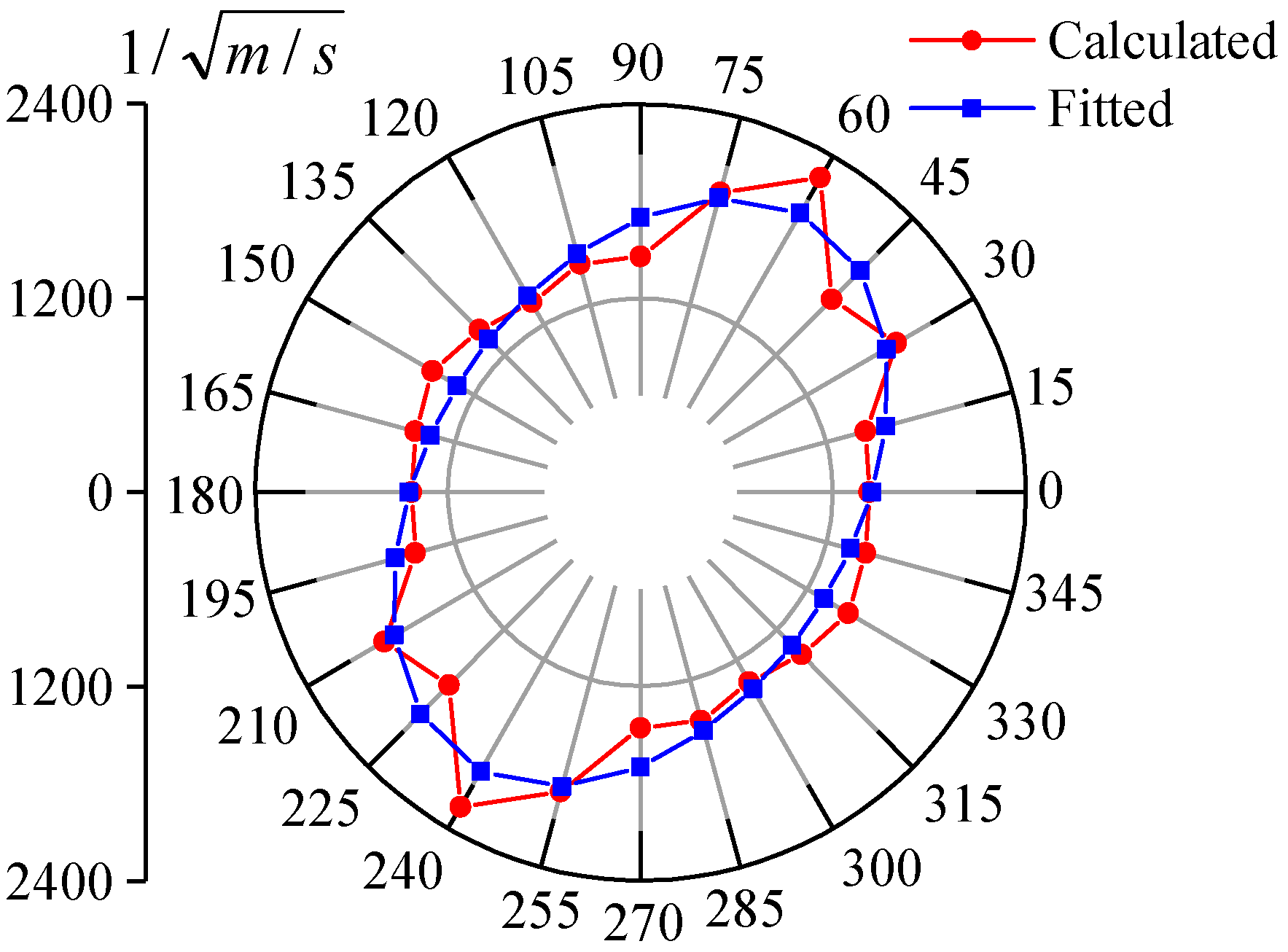
The permeability representative element volume (PREV) plays a vital role in studying groundwater seepage. Marcus [
30] pointed out that one can obtain an ellipse when drawing 1/[
K(θ)]
0.5 on a polar graph for the mean anisotropic medium. The term
K(
θ) is the permeability coefficient of the medium for a given direction
θ. In other words, if the permeability coefficient of a medium has these characteristics, the medium can be considered as a homogeneous medium. According to Marcus’s method, the PREV can be obtained by fitting the permeability coefficient with the ellipse. The standardized fitting index Root Mean Square (
RMS) evaluates the fitting performance [
31]:
where
n is the total number of fit points,
Ktensor(
θ) is the fitting value in
θ direction,
Ksim(
θ) is the hydraulic conductivity in
θ direction, and
K1 and
K2 are the lengths of the long and short axes of the fitting ellipse, which are the reciprocal of the square root of the minimum principal value and the maximum principal value of the hydraulic conductivity tensor, respectively.
If the
RMS is less than 0.2, the fitting performance is very good. The resulting hydraulic conductivity tensor can represent the permeability of the fractured rock mass, and the corresponding study area could be considered the PREV. It is assumed that the width and permeability of all fractures are the same and the evolution of permeability with time is not taken into account [
32]. The PREV values of 23 types of fractured rock mass were estimated based on the described method. The calculation process of TREV is introduced as follows, taking the fractured rock mass with low ductility and medium spacing (
Figure 3) as an example. The left and right boundary is set as the fixed water head boundary for the selected study area, and the upper and lower boundary is set as the waterproof boundary. The equivalent hydraulic conductivity can be calculated in the horizontal direction, and this can be repeated after rotating the study area to obtain the permeability in different directions, taking the study area center as the rotation center.
Figure 7 shows the fitting results when the study area is 4 m × 4 m, and the rotation angle is 15 degrees. The red circular dot line represents the conversion value of the hydraulic conductivity in 24 directions, and the blue square dot line the corresponding value in the fitting ellipse.
Figure 8 shows the variation of
RMS with increasing study area. The PREV of low ductility and medium spacing fractured rock mass is 4 m × 4 m. The PREV of the other twenty-two kinds of fractured rock mass can be calculated in the same way.
The rock masses are numbered according to the length and density of the fracture;
Figure 9 shows the PREV values of twenty-three kinds of rock mass. The abscissa represents rock type and the ordinate is the REV size. The two curves (blue and green dash line) representing PREV are very close, indicating that the generated fractures are representative and consistent with the literature [
33]. The randomness of fracture networks is the reason for the difference in PREV between this paper and the literature. The connection characteristics of fractures are different for multiple generations, although they follow the same statistical law. For certain fracture networks, the occasional connection of fractures may affect the connectivity of the whole network. This influence of the occasional connection is more obvious for rock masses with sparse fractures and where the entire fracture network is located at the edge of connection and disconnection. For sparse fracture networks, wider fracture spacing may lead to the non-existence of PREV (
Figure 9).
5. Comparison between TREV and PREV
The calculation methods for TREV and PREV of the fractured rock mass are introduced here. They are defined in order to homogenize and simplify the fractured rock mass, and reflect the scale effect of rock mass properties. The difference between them lies in their physical meaning. The TREV reflects the topological properties of the fracture network, which focuses on the topological structure and is affected by the geometric distribution and connection characteristics of fractures. The PREV focuses on the permeability of the fracture network, which is affected by the distribution and connection characteristics of the fractures. Both TREV and PREV are affected by the distribution and connection characteristics of the fractures, which provides the possibility to use TREV to estimate PREV.
The PREV of a given rock mass is a relatively fixed value. Many scholars have studied PREV based on the geometric characteristics of fractures [
17,
20]. However, little research has paid attention to the topological structure of fracture networks. After comparing TREV and PREV, we will discuss the feasibility of using TREV to estimate PREV.
Because TREV does not consider the connectivity of the fracture network, it must be modified when estimating PREV. The critical connectivity,
Nc, can be used to judge the connectivity of the fracture network, which is the average number of intersections per line [
34]. Unlike the fracture connection rate,
TB,
Nc does not consider the existence of V-nodes in the definition, and V-nodes are counted with Y-nodes. For a fracture network with fixed fracture length and equal probability distribution in two directions, the critical connectivity,
Nc, is 3.11 [
35]. The result of the connectivity judgment shows that a TREV for rocks number 3, 7, 11, and 12 does not exist.
The TREV and PREV curves have similar characteristics, and their size expands with the increase of fracture spacing for fracture networks with the same fracture length. The REV does not exist when the fracture spacing is too large. For five types of fractured rock mass with different fracture discontinuity, when the fracture spacing is very close the size of TREV and PREV is in very close proximity. When the fractures are long and the spacing is wide (rock mass numbers 22, 23, and 24), TREV size is greatly affected by accidental factors. The fracture length has little effect for fracture networks with very close fracture spacing; however, it dramatically influences fracture networks with extremely wide spacing. Comparison of the size of TREV and PREV found that they are essentially the same for the same rock. We further believe TREV can estimate PREV. Although we have studied only 23 types of rock mass, it is reasonable to believe that this method applies to all rock mass types in
Table 1. Because TREV and PREV are closer when the fracture spacing is smaller, it is reasonable to expect that this method is suitable for the unstudied rock masses in
Table 1 with extremely close fracture spacing. For the unstudied rock masses in the table with wide fracture spacing, it can be directly judged that they cannot form a connected fracture network and there is no PREV. As
Table 1 covers all kinds of fracture lengths and spacing arrangements, this method is suitable for all rock masses with an orthogonal fracture network. It should be noted that this method is not suitable for fracture permeability varying with time, because the permeability of all fractures is assumed to be the same and does not change.
Through TREV, we can obtain PREV without complex seepage calculation. TREV is only related to the topological structure of the fracture network. The estimation results obtained with this method have high credibility for many kinds of rocks discussed in this paper. However, poor performance occurs for certain cases with massive fracture spacing when the fracture network is at the edge of connectivity and disconnection. Therefore, special attention must be paid to the connectivity of a fracture network when using TREV to estimate PREV.
6. Conclusions
The topological representative element volume (TREV) is proposed based on the structural characteristics of the fracture network. Because the topological structure contains many characteristics of the fracture network, TREV can reflect comprehensive properties of the fracture network such as connectivity, continuity, etc. The feasibility of using TREV to estimate the permeability representative element volume (PREV) is discussed, and the following conclusions obtained.
(1) There is a noticeable scale effect for the topological parameter of a two-dimensional fracture network. When the study area is small, the topological parameters fluctuate violently. The variability of the topological parameters decreases gradually with the increase of the study area. When the research area is large enough, the topological parameters are stable. Therefore, topological parameters can be used as equivalent parameters for TREV.
(2) TREV considers various topological characteristics of the fracture network. After analyzing eleven topological parameters, two of them, fracture connection rate (TB) and aerial branch frequency (B20) were selected as equivalent parameters to estimate TREV. These two topological parameters are only related to the node system and can be calculated directly from the number of nodes in the fracture network.
(3) The size of TREV and PREV is essentially the same for the fractured rock discussed here. TREV is only related to the topological structure of the fracture network. Using TREV to estimate PREV can avoid complicated seepage calculation. The estimation results using this method have high credibility for many kinds of rocks. Particular attention should be paid to the connectivity of a fracture network when using TREV to estimate PREV.
The calculations in this paper focus on rock mass types with orthogonal fracture networks, which are composed of horizontal and vertical fractures. Orthogonal fracture networks are often used in related research [
35,
36] and are common in nature, including three types of squares [
37] as well as brick [
38] and pavement [
20,
39]. The Representative Element Volumes of the fractured rock masses provided in this paper (
Figure 9) represent a basis for the study of seepage in the corresponding rock masses. Based on the analysis of the topological structure and permeability characteristics of the fracture networks, the feasibility of using topological structure to study permeability is verified by the comparison of TREV and PREV. This new idea of establishes the relationship between the topological structure of fractures and their permeability through the concept of representative element volume. Similarly, future studies might attempt to study the relationship between topological structure and the mechanical properties of different rock types.


