
Investigation of Nonlinear Flow in Discrete Fracture Networks Using an Improved Hydro-Mechanical Coupling Model

Abstract
:1. Introduction
2. Laboratory Tests on Nonlinear Flow of Fractures
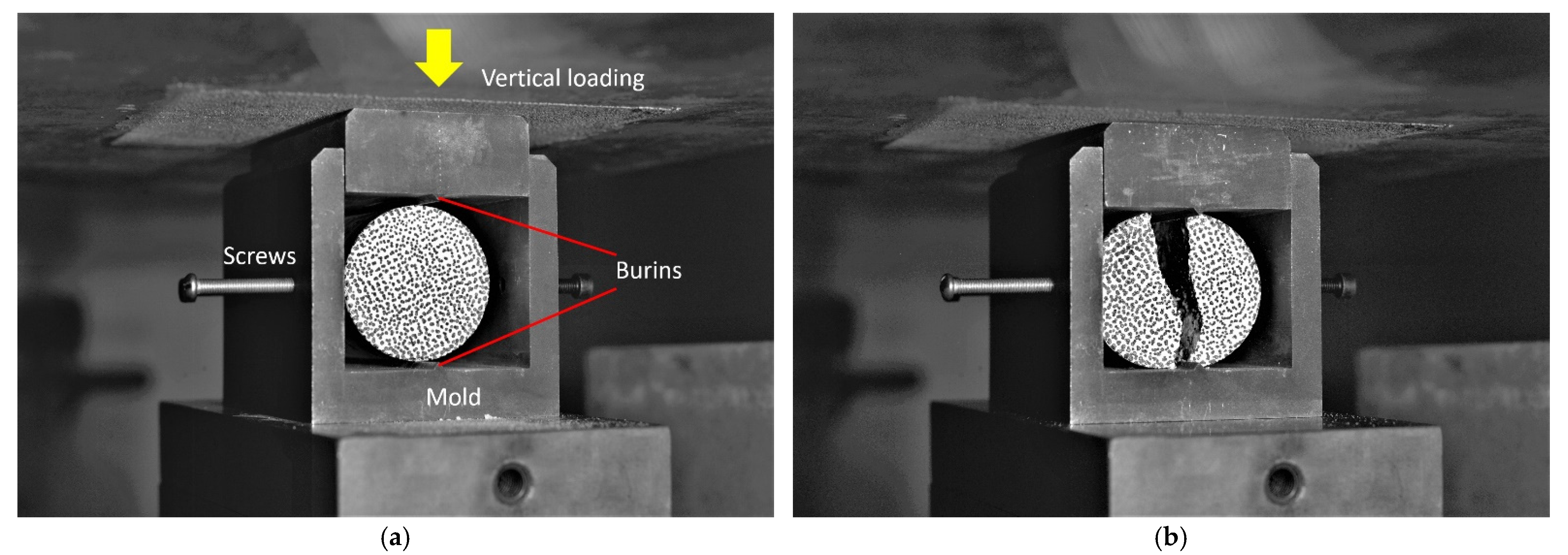
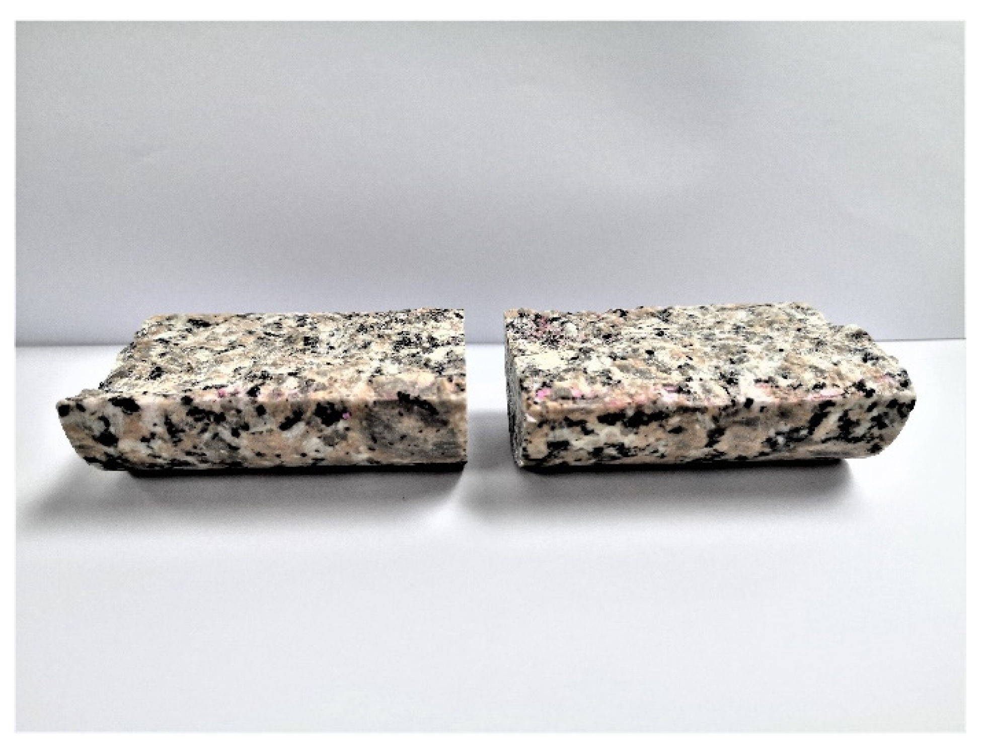
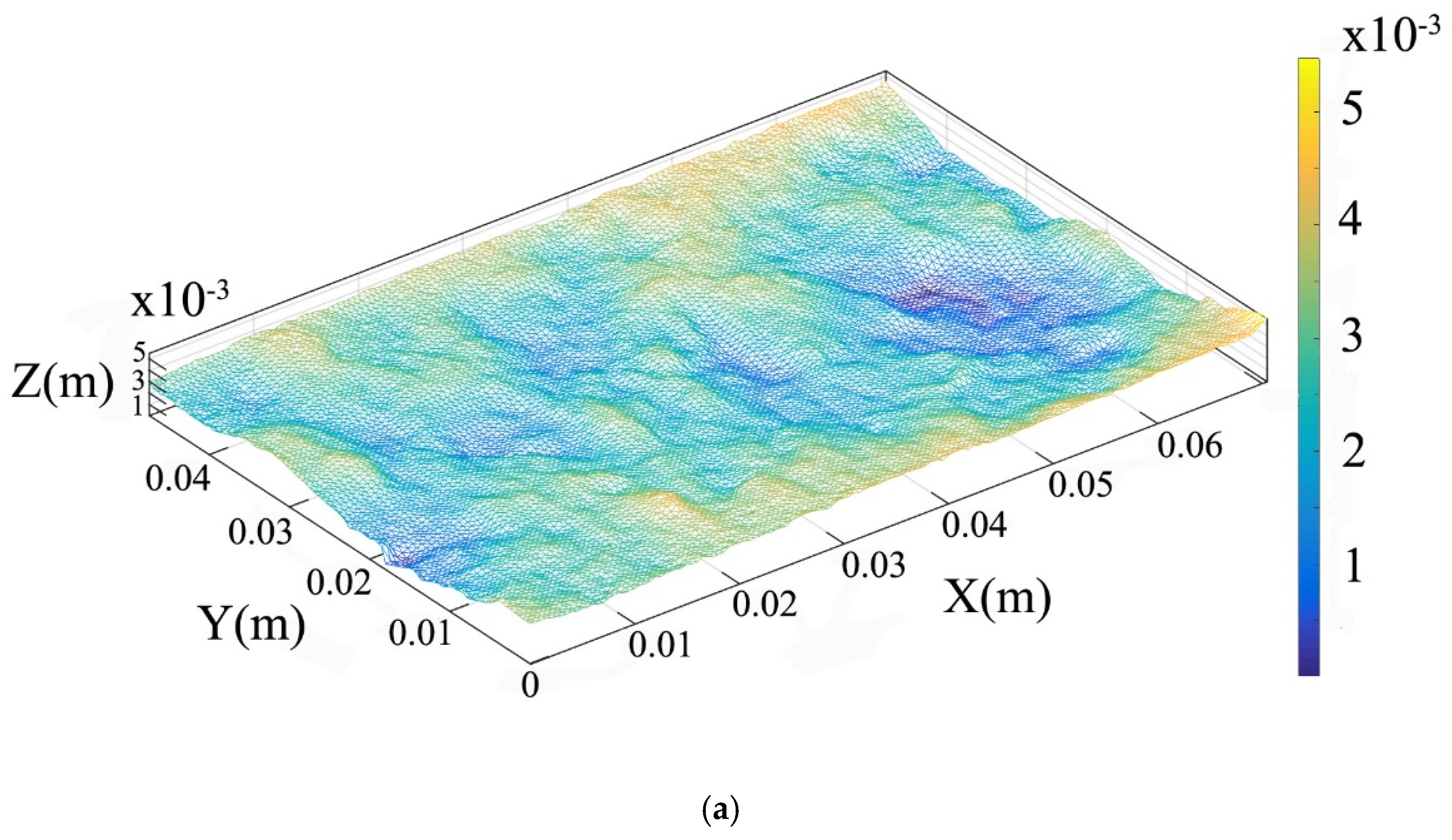
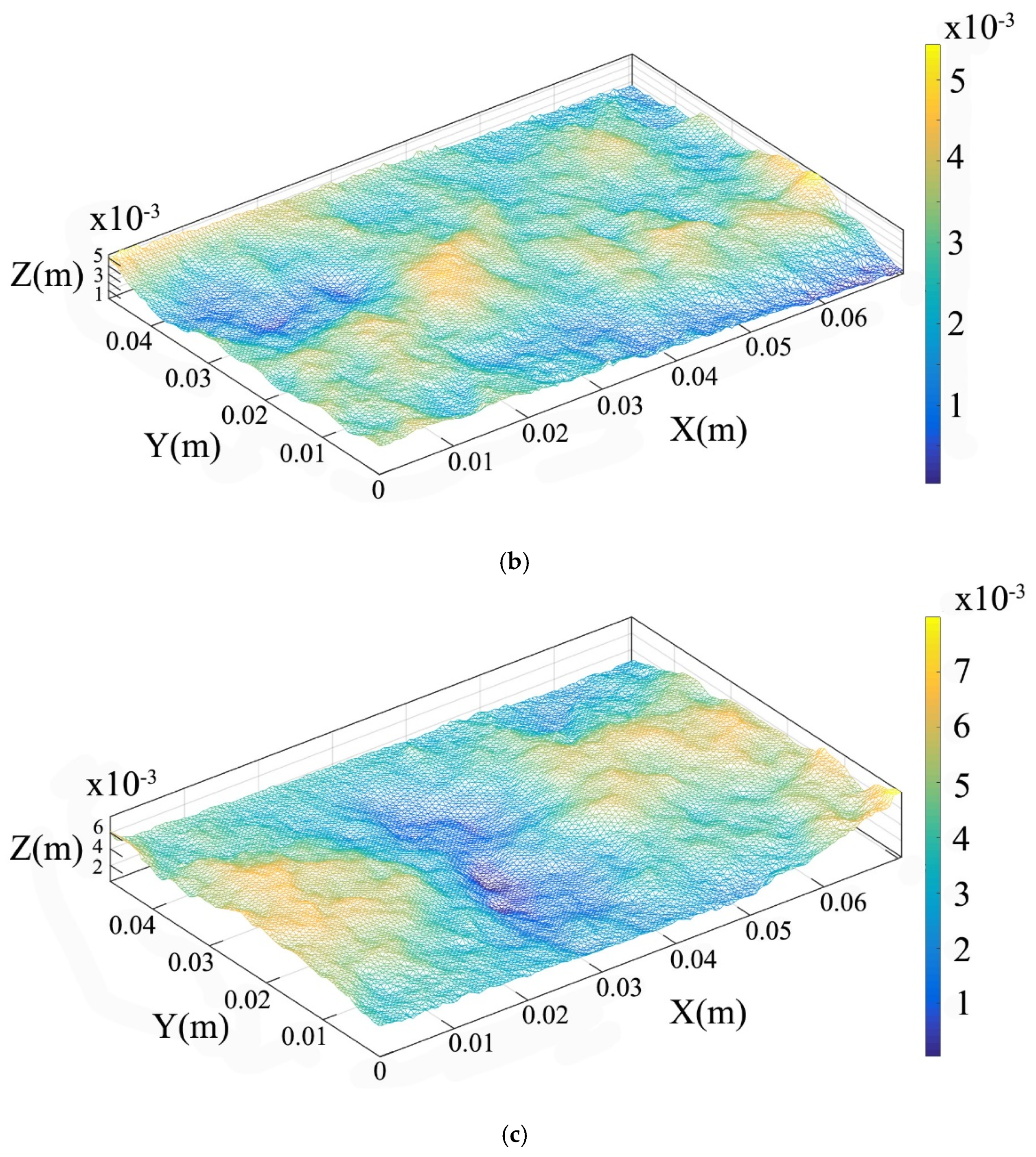
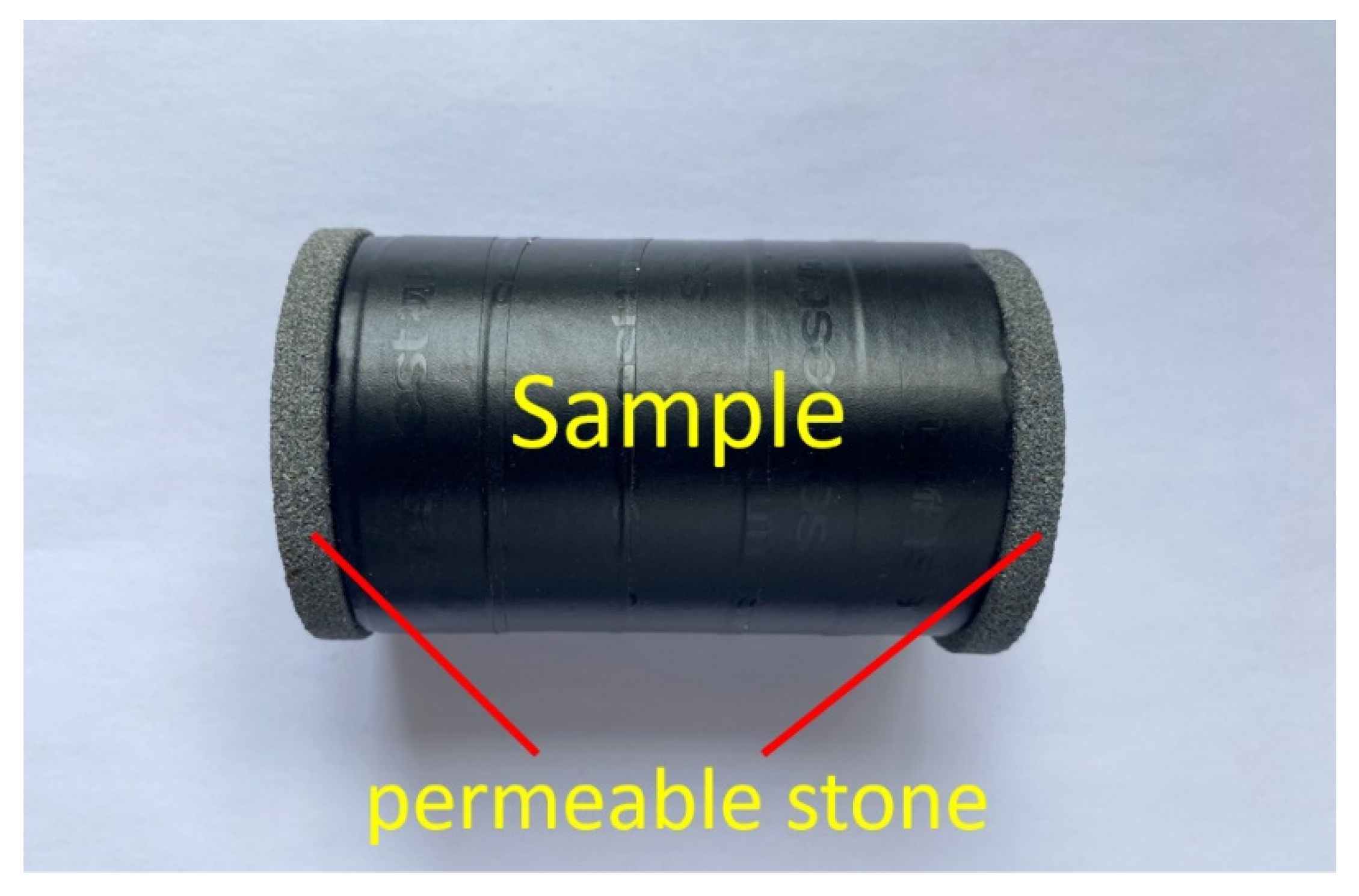
2.1. Sample Preparation
2.2. Methods and Procedures
2.3. Experimental Results and Analysis of the Nonlinear Flow of Fractures
3. Hydro-Mechanical Coupled Model for Fractured Rock Mass
3.1. Governing Equations
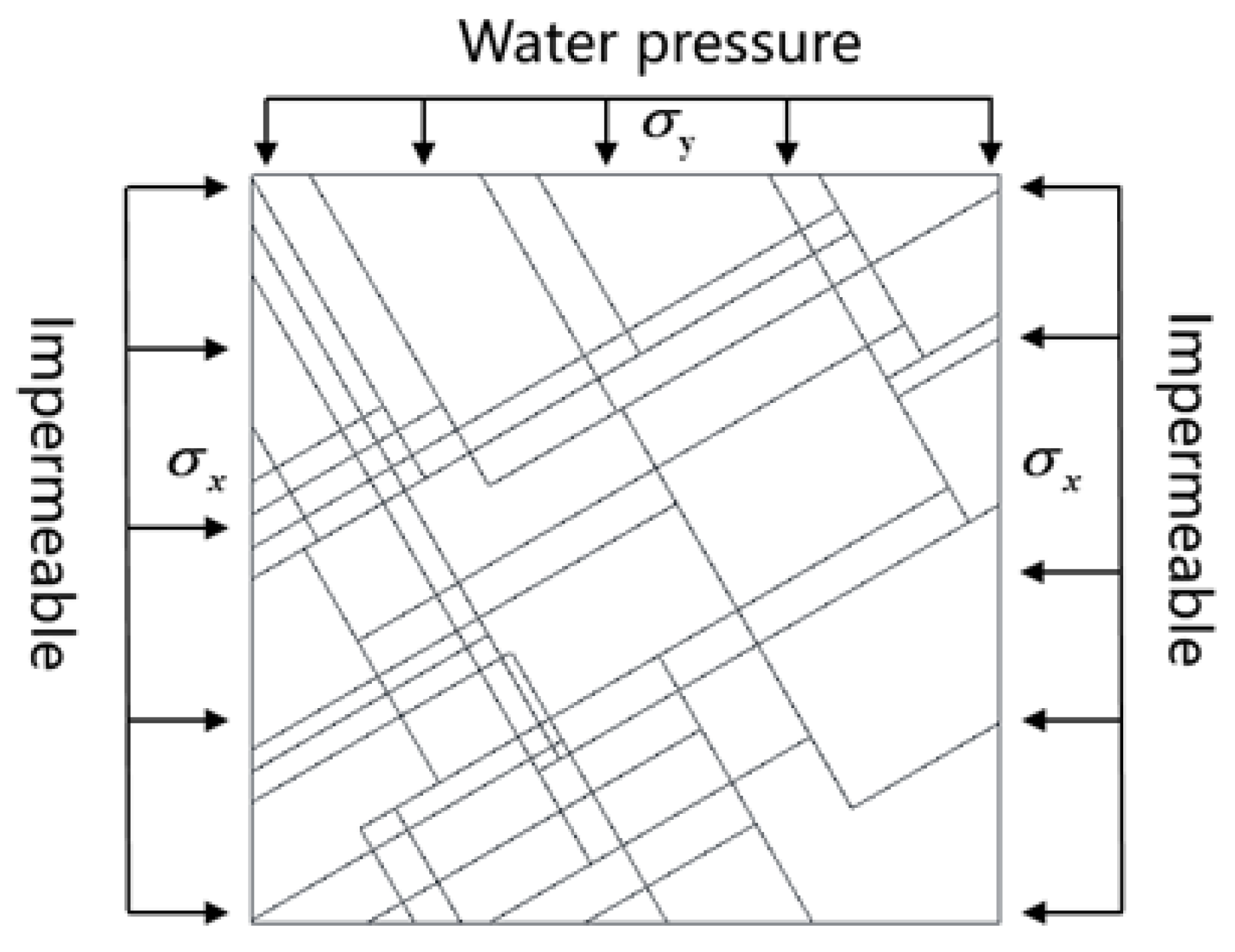
3.2. Fracture Network Generation for Rock Mass
4. Numerical Results and Discussion
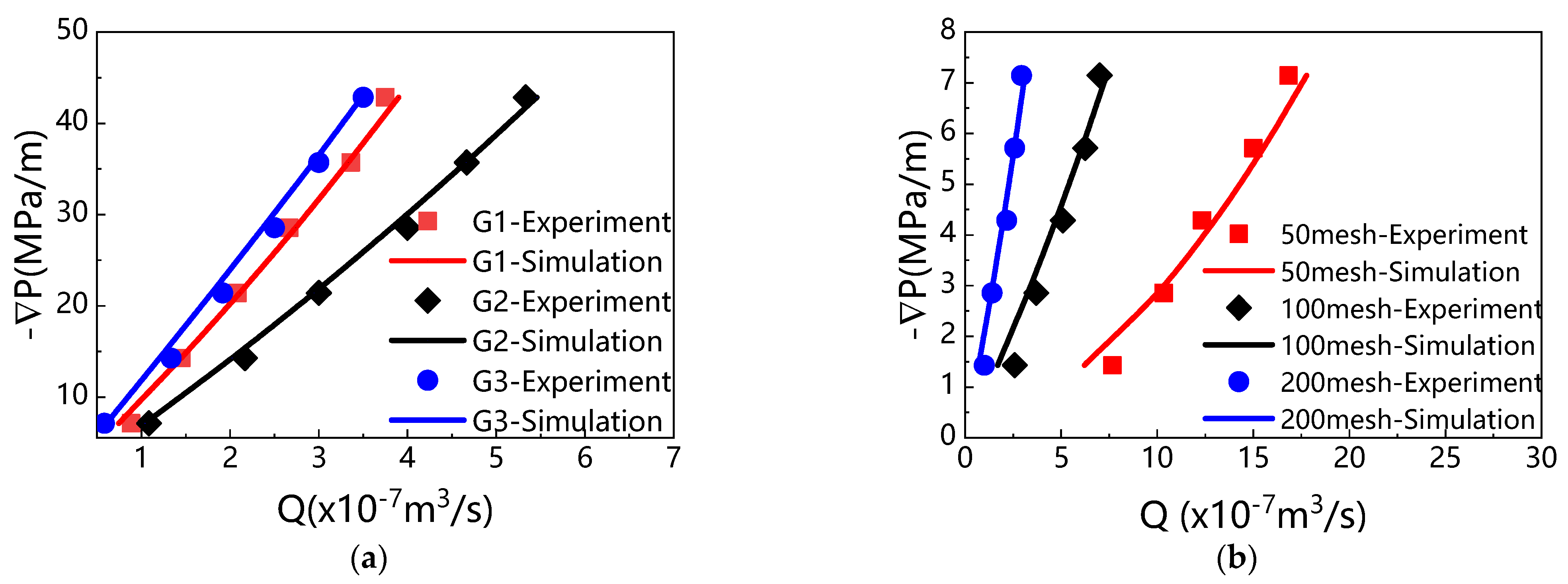
4.1. Experiment Validation
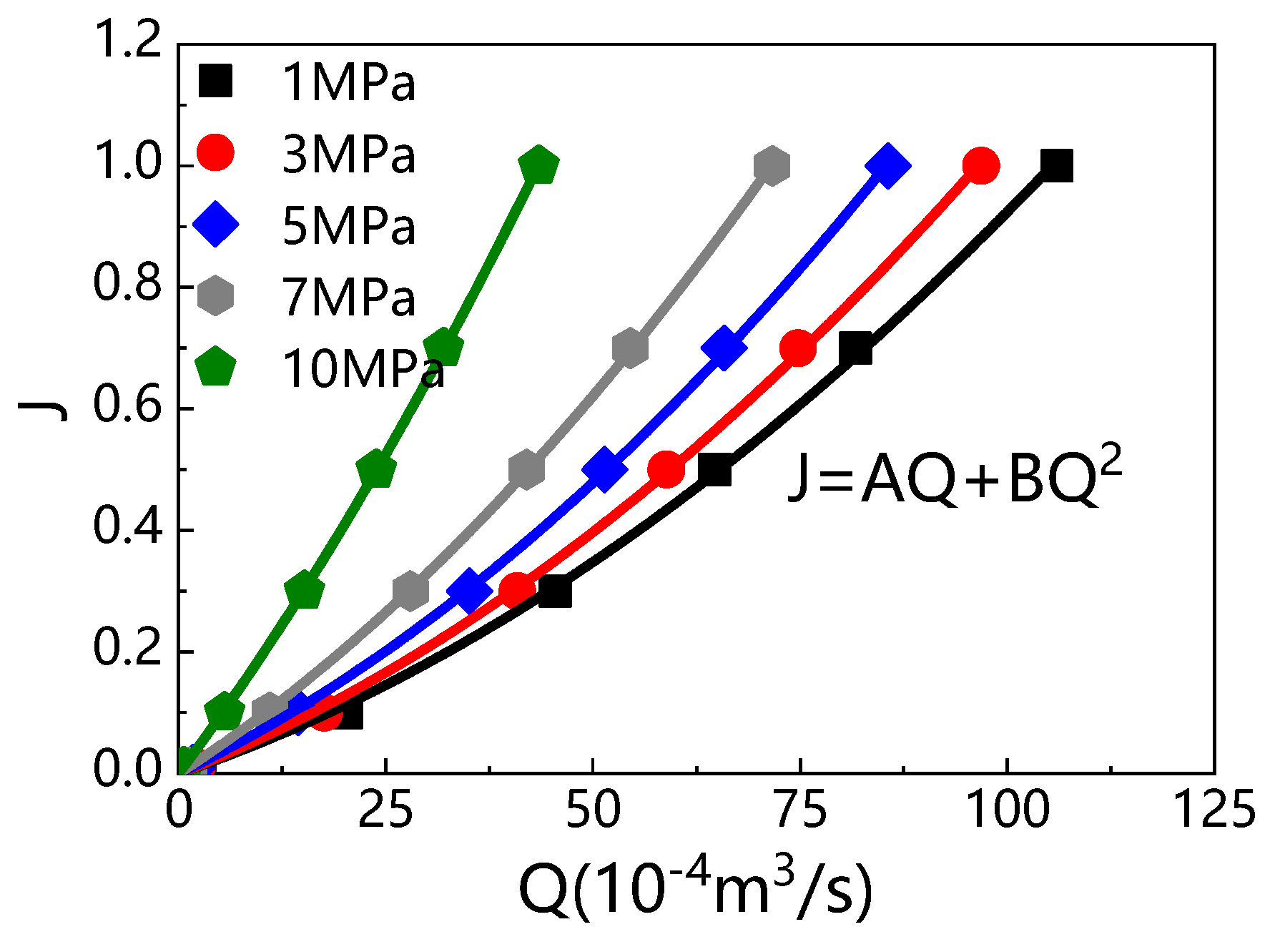
4.2. Flow Behaviours in DFNs
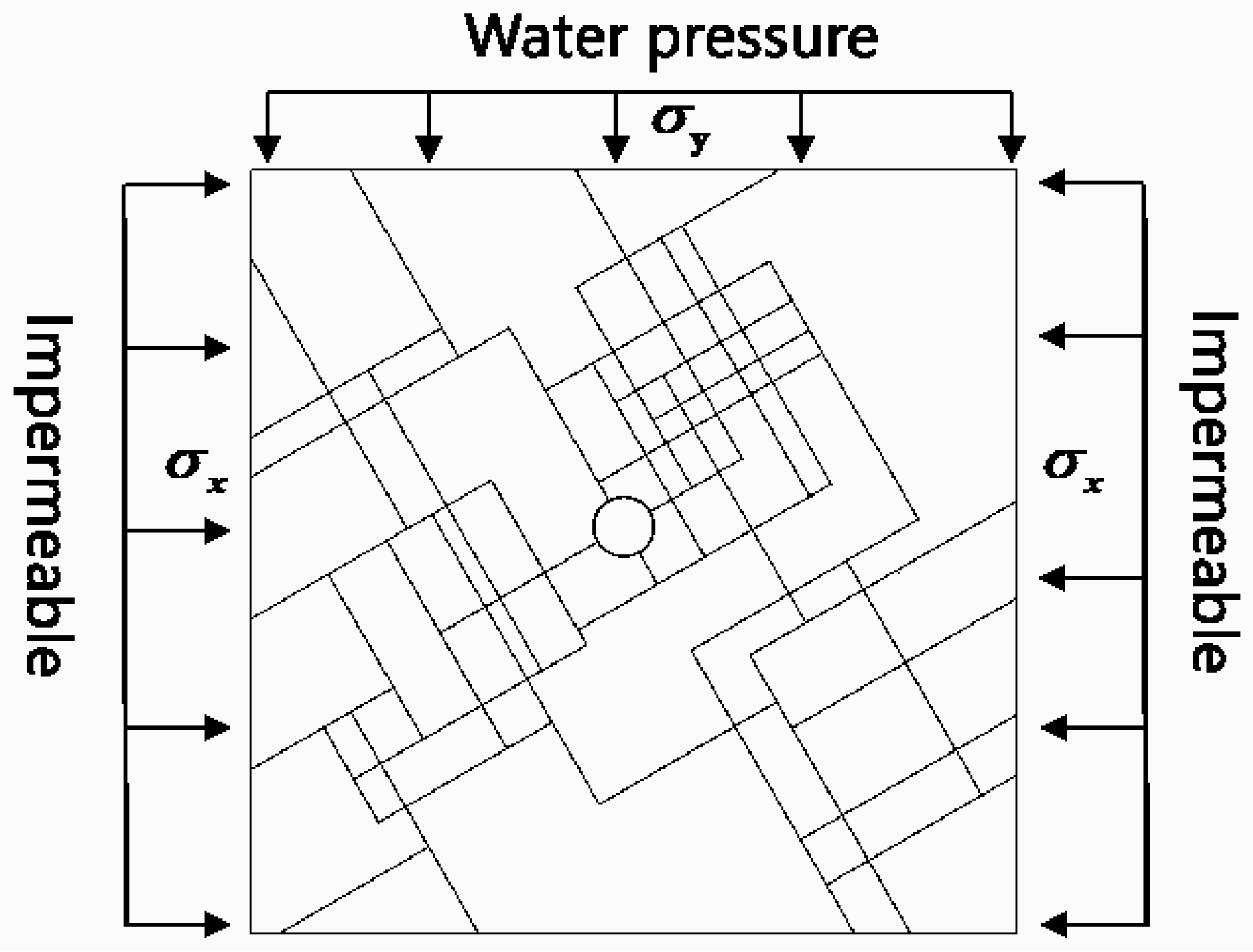
4.3. Case Study for Underground Engineering
5. Conclusions
Author Contributions
Funding
Informed Consent Statement
Data Availability Statement
Conflicts of Interest
Nomenclature
| Width of the fracture | |
| e | Aperture of the fracture |
| μ | Dynamic viscosity coefficient of the fluid |
| Volume flow | |
| ∇P | Water pressure gradient |
| A | Linear coefficient |
| Nonlinear coefficient | |
| Forchheimer coefficient | |
| Fluid density | |
| Reynolds number | |
| v | Flow velocity |
| Critical Reynolds number | |
| e0 | Initial aperture |
| Normal stress of the fracture surface | |
| Normal stiffness of the fracture | |
| K | Intrinsic permeability of fracture |
| g: | Gravitational acceleration |
| P | Water pressure |
| Hydraulic gradient | |
| KF | Forchheimer-type non-Darcy permeability |
| Surface force | |
| Physical strength | |
| Virtual strain | |
| Virtual displacement | |
| Elastic matrix | |
| Normal strain of fracture caused by water pressure | |
| Fluid pressure | |
| Compression modulus of rock mass | |
| Nodal displacement of the element | |
| Nodal pore pressure of the element | |
| Stiffness matrix | |
| Nodal force corresponding to the pore pressure of the node | |
| Volume change corresponding to node displacement | |
| G | Water storage matrix |
| F | Seepage matrix |
| Nodal load | |
| Nodal flow |
References
- Javadi, M.; Sharifzadeh, M.; Shahriar, K.; Mitani, Y. Critical Reynolds number for nonlinear flow through rough-walled fractures: The role of shear processes. Water Resour. Res. 2014, 50, 1789–1804. [Google Scholar] [CrossRef] [Green Version]
- Singh, K.K.; Singh, D.N.; Ranjith, P.G. Laboratory Simulation of Flow through Single Fractured Granite. Rock Mech. Rock Eng. 2014, 48, 987–1000. [Google Scholar] [CrossRef]
- Zhang, W.; Dai, B.B.; Liu, Z.; Zhou, C.Y. On the non-Darcian seepage flow field around a deeply buried tunnel after excavation. Bull. Eng. Geol. Environ. 2017, 78, 311–323. [Google Scholar] [CrossRef]
- Jiang, Q.H.; Ye, Z.Y.; Zhou, C.B. A numerical procedure for transient free surface seepage through fracture networks. J. Hydrol. 2014, 519, 881–891. [Google Scholar] [CrossRef]
- Ma, G.W.; Wang, H.D.; Fan, L.F.; Wang, B. Simulation of two-phase flow in horizontal fracture networks with numerical manifold method. Adv. Water Resour. 2017, 108, 293–309. [Google Scholar] [CrossRef]
- Ma, G.W.; Wang, H.D.; Fan, L.F.; Chen, Y. Segmented two-phase flow analysis in fractured geological medium based on the numerical manifold method. Adv. Water Resour. 2018, 121, 112–129. [Google Scholar] [CrossRef]
- Ma, G.W.; Wang, H.D.; Fan, L.F.; Chen, Y. A unified pipe-network-based numerical manifold method for simulating immiscible two-phase flow in geological media. J. Hydrol. 2019, 568, 119–134. [Google Scholar] [CrossRef]
- Huenges, E.; Kohl, T.; Kolditz, O.; Bremer, J.; Scheck-Wenderoth, M.; Vienken, T. Geothermal energy systems: Research perspective for domestic energy provision. Environ. Earth Sci. 2013, 70, 3927–3933. [Google Scholar] [CrossRef]
- Jiao, Y.Y.; Zhang, X.L.; Zhang, H.Q.; Li, H.B.; Yang, S.Q.; Li, J.C. A coupled thermo-mechanical discontinuum model for simulating rock cracking induced by temperature stresses. Comput. Geotech. 2015, 67, 142–149. [Google Scholar] [CrossRef]
- Fan, L.F.; Wu, Z.J.; Wan, Z.; Gao, J.W. Experimental investigation of thermal effects on dynamic behavior of granite. Appl. Therm. Eng. 2017, 125, 94–103. [Google Scholar] [CrossRef]
- Chen, Y.; Ma, G.; Wang, H. Heat extraction mechanism in a geothermal reservoir with rough-walled fracture networks. Int. J. Heat Mass Transf. 2018, 126, 1083–1093. [Google Scholar] [CrossRef]
- Chen, Y.; Ma, G.; Wang, H. The simulation of thermo-hydro-chemical coupled heat extraction process in fractured geothermal reservoir. Appl. Therm. Eng. 2018, 143, 859–870. [Google Scholar] [CrossRef]
- Ma, G.; Chen, Y.; Jin, Y.; Wang, H. Modelling temperature-influenced acidizing process in fractured carbonate rocks. Int. J. Rock Mech. Min. Sci. 2018, 105, 73–84. [Google Scholar] [CrossRef]
- Wang, G.; Wang, K.; Wang, S.G.; Elsworth, D.; Jiang, Y.J. An improved permeability evolution model and its application in fractured sorbing media. J. Nat. Gas Sci. Eng. 2018, 56, 222–232. [Google Scholar] [CrossRef]
- Tsang, C.F.; Neretnieks, I.; Tsang, Y. Hydrologic issues associated with nuclear waste repositories. Water Resour. Res. 2015, 51, 6923–6972. [Google Scholar] [CrossRef] [Green Version]
- Zhao, C.; Niu, J.L.; Zhang, Q.Z.; Zhao, C.F.; Zhou, Y.M. Failure characteristics of rock-like materials with single flaws under uniaxial compression. Bull. Eng. Geol. Environ. 2018, 78, 593–603. [Google Scholar] [CrossRef]
- Berkowitz, B. Characterizing flow and transport in fractured geological media: A review. Adv. Water Resour. 2002, 25, 861–884. [Google Scholar] [CrossRef]
- Jing, L. A review of techniques, advances and outstanding issues in numerical modelling for rock mechanics and rock engineering. Int. J. Rock Mech. Min. Sci. 2003, 40, 283–353. [Google Scholar] [CrossRef]
- Leung, C.T.O.; Zimmerman, R.W. Estimating the hydraulic conductivity of two-dimensional fracture networks using network geometric properties. Transp. Porous Media 2012, 93, 777–797. [Google Scholar] [CrossRef]
- Lang, P.S.; Paluszny, A.; Zimmerman, R.W. Permeability tensor of three-dimensional fractured porous rock and a comparison to trace map predictions. J. Geophys. Res.-Solid Earth 2014, 119, 6288–6307. [Google Scholar] [CrossRef] [Green Version]
- Cacciari, P.P.; Futai, M.M. Mapping and characterization of rock discontinuities in a tunnel using 3D terrestrial laser scanning. Bull. Eng. Geol. Environ. 2015, 75, 223–237. [Google Scholar] [CrossRef]
- Lei, Q.H.; Latham, J.P.; Tsang, C.F. The use of discrete fracture networks for modelling coupled geomechanical and hydrological behaviour of fractured rocks. Comput. Geotech. 2017, 85, 151–176. [Google Scholar] [CrossRef]
- Ye, Z.; Jiang, Q.; Zhou, C.; Liu, Y. Numerical Analysis of Unsaturated Seepage Flow in Two-Dimensional Fracture Networks. Int. J. Geomech. 2017, 17, 04016118. [Google Scholar] [CrossRef]
- Wang, L.; Chen, W.; Tan, X.; Tan, X.; Yang, J.; Yang, D.; Zhang, X. Numerical investigation on the stability of deforming fractured rocks using discrete fracture networks: A case study of underground excavation. Bull. Eng. Geol. Environ. 2020, 79, 133–151. [Google Scholar] [CrossRef]
- Tan, X.; Chen, W.; Wang, L.; Yang, J.; Tan, X. Settlement behaviors investigation for underwater tunnel considering the impacts of fractured medium and water pressure. Mar. Georesour. Geotechnol. 2020, 39, 639–648. [Google Scholar] [CrossRef]
- Barnoon, P.; Bakhshandehfard, F. Thermal management in a biological tissue in order to destroy tissue under local heating process. Case Stud. Therm. Eng. 2021, 26, 101105. [Google Scholar] [CrossRef]
- Barnoon, P. Modeling of a high temperature heat exchanger to supply hydrogen required by fuel cells through reforming process. Energy Rep. 2021, 7, 5685–5699. [Google Scholar] [CrossRef]
- Barnoon, P.; Toghraie, D.; Mehmandoust, B.; Fazilati, M.A.; Eftekhari, S.A. Comprehensive study on hydrogen production via propane steam reforming inside a reactor. Energy Rep. 2021, 7, 929–941. [Google Scholar] [CrossRef]
- Barnoon, P.; Ashkiyan, M.; Toghraie, D. Embedding multiple conical vanes inside a circular porous channel filled by two-phase nanofluid to improve thermal performance considering entropy generation. Int. Commun. Heat Mass Transf. 2021, 124, 105209. [Google Scholar] [CrossRef]
- Barnoon, P.; Toghraie, D.; Mehmandoust, B.; Fazilati, M.A.; Eftekhari, S.A. Natural-forced cooling and Monte-Carlo multi-objective optimization of mechanical and thermal characteristics of a bipolar plate for use in a proton exchange membrane fuel cell. Energy Rep. 2022, 8, 2747–2761. [Google Scholar] [CrossRef]
- Wang, L.; Chen, W.; Vuik, C. Hybrid-dimensional modeling for fluid flow in heterogeneous porous media using dual fracture-pore model with flux interaction of fracture-cavity network. J. Nat. Gas Sci. Eng. 2022, 100, 104450. [Google Scholar] [CrossRef]
- Min, K.B.; Rutqvist, J.; Tsang, C.F.; Jing, L.R. Stress-dependent permeability of fractured rock masses: A numerical study. Int. J. Rock Mech. Min. Sci. 2004, 41, 1191–1210. [Google Scholar] [CrossRef] [Green Version]
- Kumara, C.; Indraratna, B. Normal Deformation and Formation of Contacts in Rough Rock Fractures and Their Influence on Fluid Flow. Int. J. Geomech. 2016, 17, 04016022. [Google Scholar] [CrossRef]
- Kamali, A.; Pournik, M. Fracture closure and conductivity decline modeling-application in unpropped and acid etched fractures. J. Unconv. Oil Gas Res. 2016, 14, 44–55. [Google Scholar] [CrossRef]
- Selvadurai, A.P.S. In-plane loading of a bonded rigid disc embedded at a pre-compressed elastic interface: The role of non-linear interface responses. Mech. Syst. Signal Process. 2020, 144, 106871. [Google Scholar] [CrossRef]
- Vogler, D.; Amann, F.; Bayer, P.; Elsworth, D. Permeability evolution in natural fractures subject to cyclic loading and gouge formation. Rock Mech. Rock Eng. 2016, 49, 3463–3479. [Google Scholar] [CrossRef]
- Selvadurai, A.P.S.; Głowacki, A. Stress-Induced Permeability Alterations in an Argillaceous Limestone. Rock Mech. Rock Eng. 2017, 50, 1079–1096. [Google Scholar] [CrossRef]
- Vilarrasa, V.; Koyama, T.; Neretnieks, I.; Jing, L. Shear-induced flow channels in a single rock fracture and their effect on solute transport. Transp. Porous Media 2011, 87, 503–523. [Google Scholar] [CrossRef]
- Mofakham, A.A.; Stadelman, M.; Ahmadi, G.; Shanley, K.T.; Crandall, D. Computational Modeling of Hydraulic Properties of a Sheared Single Rock Fracture. Transp. Porous Media 2018, 124, 1–30. [Google Scholar] [CrossRef]
- Chen, Y.D.; Liang, W.G.; Selvadurai, A.P.S.; Zhao, Z.H. Influence of asperity degradation and gouge formation on flow during rock fracture shearing. Int. J. Rock Mech. Min. Sci. 2021, 143, 104795. [Google Scholar] [CrossRef]
- Klimczak, C.; Schultz, R.A.; Parashar, R.; Reeves, D.M. Cubic law with aperture-length correlation: Implications for network scale fluid flow. Hydrogeol. J. 2010, 18, 851–862. [Google Scholar] [CrossRef]
- Rasouli, V.; Hosseinian, A. Correlations developed for estimation of hydraulic parameters of rough fractures through the simulation of JRC flow channels. Rock Mech. Rock Eng. 2011, 44, 447–461. [Google Scholar] [CrossRef]
- Xiong, X.B.; Li, B.; Jiang, Y.J.; Koyama, T.; Zhang, C.H. Experimental and numerical study of the geometrical and hydraulic characteristics of a single rock fracture during shear. Int. J. Rock Mech. Min. Sci. 2011, 48, 1292–1302. [Google Scholar] [CrossRef]
- Rezaei Niya, S.M.; Selvadurai, A.P.S. Correlation of joint roughness coefficient and permeability of a fracture. Int. J. Rock Mech. Min. Sci. 2019, 113, 150–162. [Google Scholar] [CrossRef]
- Javadi, M.; Sharifzadeh, M.; Shahriar, K. A new geometrical model for non-linear fluid flow through rough fractures. J. Hydrol. 2010, 389, 18–30. [Google Scholar] [CrossRef]
- Quinn, P.M.; Cherry, J.A.; Parker, B.L. Quantification of non-Darcian flow observed during packer testing in fractured sedimentary rock. Water Resour. Res. 2011, 47, W09533. [Google Scholar] [CrossRef]
- Liu, R.C.; Huang, N.; Jiang, Y.J.; Jing, H.W.; Yu, L.Y. A numerical study of shear-induced evolutions of geometric and hydraulic properties of self-affine rough-walled rock fractures. Int. J. Rock Mech. Min. Sci. 2020, 127, 104211. [Google Scholar] [CrossRef]
- Quinn, P.M.; Parker, B.L.; Cherry, J.A. Using constant head step tests to determine hydraulic apertures in fractured rock. J. Contam. Hydrol. 2011, 126, 85–99. [Google Scholar] [CrossRef]
- Cherubini, C.; Giasi, C.I.; Pastore, N. Bench scale laboratory tests to analyze non-linear flow in fractured media. Hydrol. Earth Syst. Sci. 2012, 9, 5575–5609. [Google Scholar] [CrossRef] [Green Version]
- Liu, R.C.; Li, B.; Jiang, Y.J. Critical hydraulic gradient for nonlinear flow through rock fracture networks: The roles of aperture, surface roughness, and number of intersections. Adv. Water Resour. 2016, 88, 53–65. [Google Scholar] [CrossRef]
- Wang, M.; Chen, Y.F.; Ma, G.W.; Zhou, J.Q.; Zhou, C.B. Influence of surface roughness on nonlinear flow behaviors in 3D self-affine rough fractures: Lattice Boltzmann simulations. Adv. Water Resour. 2016, 96, 373–388. [Google Scholar] [CrossRef]
- Fan, L.F.; Wang, H.D.; Wu, Z.J.; Zhao, S.H. Effects of angle patterns at fracture intersections on fluid flow nonlinearity and outlet flow rate distribution at high Reynolds numbers. Int. J. Rock Mech. Min. Sci. 2019, 124, 104136. [Google Scholar] [CrossRef]
- Chen, Y.F.; Zhou, J.Q.; Hu, S.H.; Hu, R.; Zhou, C.B. Evaluation of Forchheimer equation coefficients for non-Darcy flow in deformable rough-walled fractures. J. Hydrol. 2015, 529, 993–1006. [Google Scholar] [CrossRef]
- Zhou, J.Q.; Hu, S.H.; Fang, S.; Chen, Y.F.; Zhou, C.B. Nonlinear flow behavior at low Reynolds numbers through rough-walled fractures subjected to normal compressive loading. Int. J. Rock Mech. Min. Sci. 2015, 80, 202–218. [Google Scholar] [CrossRef]
- Xiong, F.; Jiang, Q.; Xu, C.; Zhang, X.; Zhang, Q. Influences of connectivity and conductivity on nonlinear flow behaviours through three-dimension discrete fracture networks. Comput. Geotech. 2019, 107, 128–141. [Google Scholar] [CrossRef]
- Rong, G.; Yang, J.; Cheng, L.; Zhou, C.B. Laboratory investigation of nonlinear flow characteristics in rough fractures during shear process. J. Hydrol. 2016, 541, 1385–1394. [Google Scholar] [CrossRef]
- Yin, Q.; Ma, G.W.; Jing, H.W.; Wang, H.D.; Su, H.J.; Wang, Y.C.; Liu, R.C. Hydraulic properties of 3D rough-walled fractures during shearing: An experimental study. J. Hydrol. 2017, 555, 169–184. [Google Scholar] [CrossRef]
- Zou, L.; Jing, L.; Cvetkovic, V. Shear-enhanced nonlinear flow in rough-walled rock fractures. Int. J. Rock Mech. Min. Sci. 2017, 97, 33–45. [Google Scholar] [CrossRef] [Green Version]
- Yang, Z.Y.; Lo, S.C.; Di, C.C. Reassessing the joint roughness cofficient (JRC) estimation using Z2. Rock Mech. Rock Eng. 2001, 34, 243–251. [Google Scholar] [CrossRef]
- Yong, R.; Ye, J.; Li, B.; Du, S.G. Determining the maximum sampling interval in rock joint roughness measurements using Fourier series. Int. J. Rock Mech. Min. Sci. 2018, 101, 78–88. [Google Scholar] [CrossRef]
- Ladanyi, B.; Archambault, G. Shear strength and Deformability of Filled Indented Joints. In Proceedings of the International Symposium on the Geotechnics of Structurally Complex Formations, Capri, Italy, 19–21 September 1977. [Google Scholar]
- Sui, Q.; Yang, D.S.; Chen, W.Z.; Yang, S.Q. Experimental investigation on the transmissivity of fractured granite filled with different materials. Bull. Eng. Geol. Environ. 2022, 81, 1. [Google Scholar] [CrossRef]
- Zimmerman, R.W.; Bodvarsson, G.S. Hydraulic conductivity of rock fractures. Transp. Porous Media 1996, 23, 1–30. [Google Scholar] [CrossRef] [Green Version]
- Bear, J. Dynamics of Fluids in Porous Media; Am. Elsevier: New York, NY, USA, 1972. [Google Scholar]
- Zimmerman, R.W.; Al-Yaarubi, A.; Pain, C.C.; Grattoni, C.A. Non-linear regimes of fluid flow in rock fractures. Int. J. Rock Mech. Min. Sci. 2004, 41, 163–169. [Google Scholar] [CrossRef]
- Zeng, Z.; Grigg, R. A criterion for non-Darcy flow in porous media. Transp. Porous Media 2006, 63, 57–69. [Google Scholar] [CrossRef]
- Heuze, F.E. Dilatant effects of rock joints. In Proceedings of the 4th ISRM Congress, Montreux, Switzerland, 2–8 September 1979. [Google Scholar]
- Johnston, I.W.; Lam, T.S.K.; Williams, A.F. Constant normal stiffness direct shear testing for socketed pile design in weak rock. Geotechnique 1987, 37, 83–89. [Google Scholar] [CrossRef]
- Snow, D.T. A Parallel Plate Model of Fractured Permeable Media. Ph.D. Thesis, University of California, Berkeley, CA, USA, 1965. [Google Scholar]
- Wang, J.; Tsang, C.F.; Sterbentz, R.A. The state of the art of numerical modeling of thermohydrologic flow in fractured rock masses. Environ. Geol. 1982, 4, 133–199. [Google Scholar] [CrossRef] [Green Version]
- Xu, K.; Lei, X.W.; Meng, Q.S.; Zhou, X.B. Study of inertial coefficient of non-Darcy seepage flow. Chin. J. Rock Mech. Eng. 2012, 31, 164–170. [Google Scholar]
- Veyskarami, M.; Hassani, A.H.; Ghazanfari, M.H. Modeling of non-Darcy flow through anisotropic porous media: Role of pore space profiles. Chem. Eng. Sci. 2016, 151, 93–104. [Google Scholar] [CrossRef]
- Chen, W.Z.; Wu, G.J.; Jia, S.P. The Application of Abaqus in Tunnel and Underground Works; Water Power Press: Beijing, China, 2010. [Google Scholar]
- Li, B.; Liu, R.C.; Jiang, Y.J. Influences of hydraulic gradient, surface roughness, intersecting angle, and scale effect on nonlinear flow behavior at single fracture intersections. J. Hydrol. 2016, 538, 440–453. [Google Scholar] [CrossRef]
- Liu, R.C.; Li, B.; Jiang, Y.J.; Yu, L.Y. Experimental and numerical study of hydraulic properties of 3D crossed fractures. Chin. J. Rock Mech. Eng. 2016, 35, 3813–3821. [Google Scholar] [CrossRef]


| Sample | Diameter (mm) | Length (mm) | Filling Conditions (mesh) | Water Pressure (MPa) | |
|---|---|---|---|---|---|
| Case 1 | G 1 | 47.92 | 70.52 | / | 0.5–3.0 |
| Case 2 | 50 | 0.1–0.5 | |||
| Case 3 | 100 | ||||
| Case 4 | 200 | ||||
| Case 5 | G 2 | 47.88 | 70.67 | / | 0.5–3.0 |
| Case 6 | 50 | 0.1–0.5 | |||
| Case 7 | 100 | ||||
| Case 8 | 200 | ||||
| Case 9 | G 3 | 47.65 | 70.32 | / | 0.5–3.0 |
| Case 10 | 50 | 0.1–0.5 | |||
| Case 11 | 100 | ||||
| Case 12 | 200 |
| Filling Condition | Sample | Linear Coefficient A | Nonlinear Coefficient B | R2 |
|---|---|---|---|---|
| With 50 mesh particles | G1 | 3.02 × 10⁵ | 1.69 × 10¹² | >0.99 |
| G2 | 3.10 × 10⁶ | 2.37 × 10¹² | >0.99 | |
| G3 | 3.50 × 10⁵ | 2.34 × 10¹² | >0.99 | |
| With 100 mesh particles | G1 | 8.80 × 10⁵ | 1.87 × 10¹² | >0.99 |
| G2 | 4.94 × 10⁶ | 2.61 × 10¹² | >0.99 | |
| G3 | 3.91 × 10⁶ | 8.81 × 10¹² | >0.99 | |
| With 200 mesh particles | G1 | 1.72 × 10⁶ | 2.13 × 10¹³ | >0.99 |
| G2 | 1.01 × 10⁷ | 1.57 × 10¹³ | >0.99 | |
| G3 | 1.21 × 10⁷ | 4.03 × 10¹³ | >0.99 | |
| No filling | G1 | 8.60 × 10⁷ | 7.14 × 10¹³ | >0.99 |
| G2 | 5.70 × 10⁷ | 4.22 × 10¹³ | >0.99 | |
| G3 | 1.01 × 10⁸ | 6.07 × 10¹³ | >0.99 |
| Fracture Section | Length (cm) | Aperture (mm) | Width (cm) |
|---|---|---|---|
| 1 | 5.78 | 0.6 | 10 |
| 2 | 5.78 | 0.3 | 10 |
| 3 | 5.78 | 0.3 | 10 |
| 4 | 5.78 | 0.6 | 10 |
| 5 | 10 | 1 | 10 |
| Cases | Inlet (s) | Outlet (s) | Remarks |
|---|---|---|---|
| Case 1 | 1 | 2 | One inlet and one outlet |
| Case 2 | 1 | 1,2 | One inlet and two outlets |
| Case 3 | 1,2 | 2 | Two inlets and one outlet |
| Case 4 | 1,2 | 1,2 | Two inlets and two outlets |
| Mean Value (Expectation) | Standard Variance | |
|---|---|---|
| Trace length (m) | 15 | 4 |
| 15 | 2 | |
| Dip (°) | 30 | 5 |
| 120 | 7 | |
| Spacing | Random distribution | |
| Elastic Modulus | Normal Stiffness | Cohesion | Friction Angle | Poisson’s Ratio | Density | |
|---|---|---|---|---|---|---|
| Matrix | 10 GPa | / | 1.6 MPa | 45° | 0.3 | 2000 kg/m3 |
| Fractures | / | 40 MPa/mm | / | / | 0.25 | 1500 kg/m3 |
| Mean Value (Expectation) | Standard Variance | |
|---|---|---|
| Trace length (m) | 20 | 4 |
| 18 | 2 | |
| Dip (°) | 30 | 5 |
| 120 | 7 | |
| Spacing | Random distribution | |
| Elastic Modulus | Normal Stiffness | Cohesion | Friction Angle | Poisson’s Ratio | Density | |
|---|---|---|---|---|---|---|
| Matrix | 10 GPa | / | 1.5 MPa | 42° | 0.27 | 2150 kg/m3 |
| Fractures | / | 40 MPa/mm | / | / | 0.25 | 1850 kg/m3 |
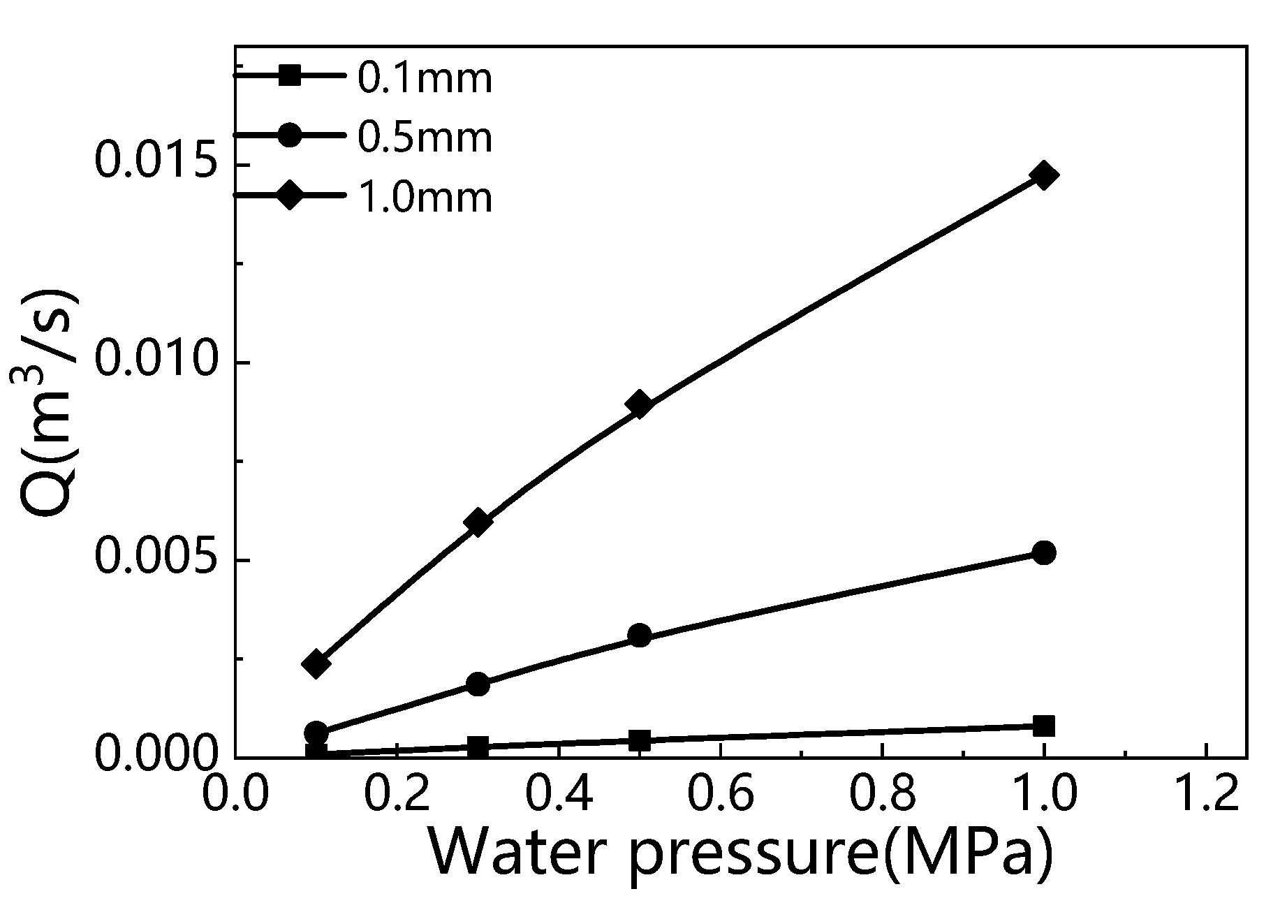
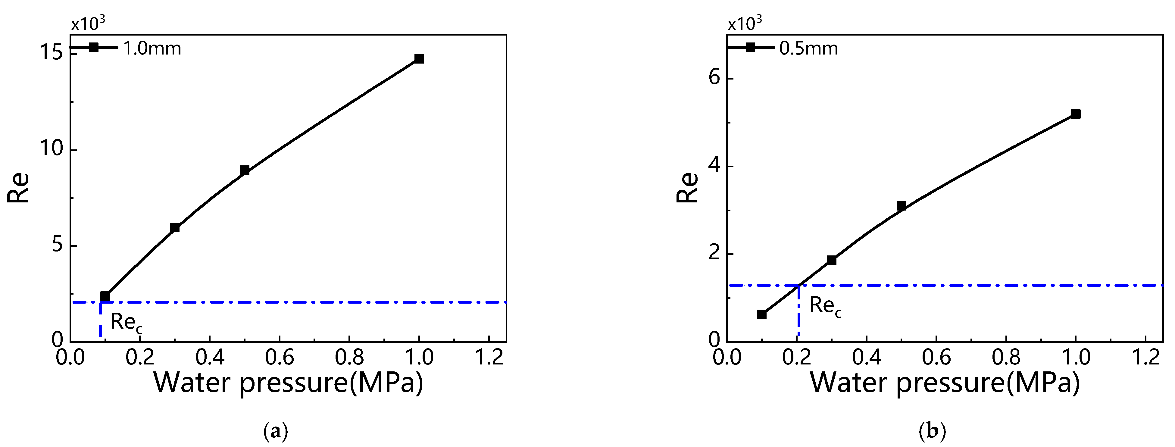
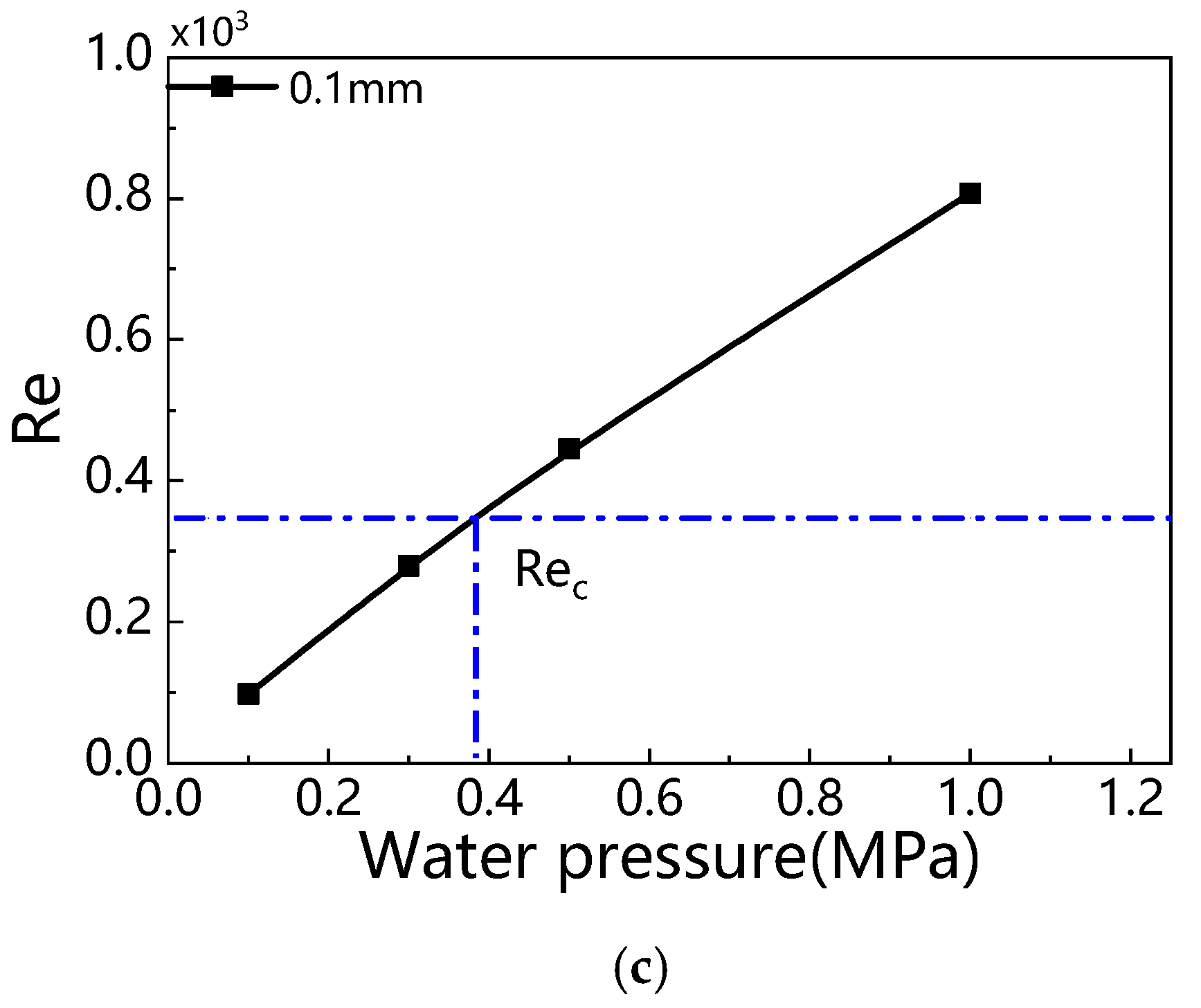
| Fracture Aperture (mm) | Water Pressure (MPa) | Flow (m3/s) | Reynolds Number | Critical Reynolds Number |
|---|---|---|---|---|
| 0.1 | 0.1 | 9.77 × 10⁻⁵ | 98 | 347 |
| 0.3 | 2.79 × 10⁻⁴ | 279 | ||
| 0.5 | 4.46 × 10⁻⁴ | 446 | ||
| 1.0 | 8.07 × 10⁻⁴ | 807 | ||
| 0.5 | 0.1 | 6.26 × 10⁻⁴ | 626 | 1288 |
| 0.3 | 1.86 × 10⁻³ | 1863 | ||
| 0.5 | 3.10 × 10⁻³ | 3100 | ||
| 1.0 | 5.19 × 10⁻³ | 5191 | ||
| 1.0 | 0.1 | 2.39 × 10⁻³ | 2386 | 2072 |
| 0.3 | 5.96 × 10⁻³ | 5960 | ||
| 0.5 | 8.95 × 10⁻³ | 8950 | ||
| 1.0 | 1.47 × 10⁻² | 14,740 |
Publisher’s Note: MDPI stays neutral with regard to jurisdictional claims in published maps and institutional affiliations. |
© 2022 by the authors. Licensee MDPI, Basel, Switzerland. This article is an open access article distributed under the terms and conditions of the Creative Commons Attribution (CC BY) license (https://creativecommons.org/licenses/by/4.0/).
Share and Cite
Sui, Q.; Chen, W.; Wang, L. Investigation of Nonlinear Flow in Discrete Fracture Networks Using an Improved Hydro-Mechanical Coupling Model. Appl. Sci. 2022, 12, 3027. https://doi.org/10.3390/app12063027
Sui Q, Chen W, Wang L. Investigation of Nonlinear Flow in Discrete Fracture Networks Using an Improved Hydro-Mechanical Coupling Model. Applied Sciences. 2022; 12(6):3027. https://doi.org/10.3390/app12063027
Chicago/Turabian StyleSui, Qun, Weizhong Chen, and Luyu Wang. 2022. "Investigation of Nonlinear Flow in Discrete Fracture Networks Using an Improved Hydro-Mechanical Coupling Model" Applied Sciences 12, no. 6: 3027. https://doi.org/10.3390/app12063027