Applying ANN and TM to Build a Prediction Model for the Site Selection of a Convenience Store

Abstract

This article builds a systematic and reliable site selection prediction model for a chain of convenience stores (CVSs) to improve the existing decision method of using experienced managers to select sites. Specifically, this study used an artificial neural network (ANN) technique—back-propagation neural network (BPN)—to build the prediction model. To achieve optimization in executing the BPN, the Taguchi method (TM) was adopted to find the optimal parameters for the BPN. The actual data from a chain of CVSs was employed to validate the model. The results indicated that the prediction accuracy rate and decision quality of the proposed model were higher than those of the existing manager-directed decision method. With intense retail competition, the accurate determination of the location of a new convenience store (CVS) is vital to its success. This study asserts that with systematic and scientific assessment, the site selection decision for new chain CVSs will be less human-biased in nature if the prediction model is used as an auxiliary decision-making tool.

1. Introduction

In general, the selection of the site of a new retail store is markedly different from the selection of a site for manufacturing facilities. The decision over the latter is primarily focused on cost minimization. Retail stores, however, generally seek to maximize revenues.

A review of the limited literature on store site selection revealed that most germane studies use the following methods for site selection: analytic network process (ANP) [1,2], analytic hierarchy process (AHP) [3,4], quantitative methods, such as regression models [5], and weighted scores with the use of checklists [6]. This previous work mainly attempts to identify the influencing factors and obtain the weights of these influencing factors when establishing new stores. In addition, the results of these investigations provide limited assistance vis-à-vis the practical site selection problem. In recent years, use of artificial neural networks (ANNs) for site selection has been shown to be especially effective in various venues, such as the locations of wind farms [7], landfills [8], water waste [9], and CVSs [10]. Currently, the selection of a specific site is comprehensive in practice. The location selection techniques that use ANNs solve the problem for a region but not for a specific site. Therefore, the results obtained from an ANN are not comprehensive, and the reference value they provide is limited.

Our study employed an ANN technique—a back-propagation neural network (BPN)—to generate suitable CVS site selection criteria from various inputs collected from a well-known CVS chain in Taiwan. To establish a set of robust site selection prediction models with the BPN, the Taguchi method (TM) [11] was adopted to identify the optimal parameters for performing the BPN.

2. Literature Review

Site selection is a crucial decision for most businesses, including those in retailing, the service industry, and manufacturing [12]. It has a consequential impact on profitability and is a valuable strategic tool for chain store operations. Site selection involves more than merely selecting a site with good visibility and accessibility [13]; accordingly, it requires a thorough evaluation process.

Competition, demographics (i.e., prospective customers in the area), and market demands must also be considered [14]. For example, a site requires an adequate number of vehicles to pass by each day. Additionally, the availability of convenient parking is often an essential consideration, well as the definition and evaluation of competition near the proposed site. In fact, the number of competitors near a site can be a double-edged sword: competitors may attract crowds to the area yet also offer severe competition [15]. There may also be neighborhood changes, traffic changes, natural barriers, and human-made obstacles at the site [16]. Therefore, a robust and systematic design system for a store’s, site selection is essential, especially because of the dynamism in the store and business environments.

In addition to the above issues, the impact of site location on a firm’s financial metrics is important. Ganesha et al. [17] and Aversa et al. [18] investigated the variance in store performance with respect to customer expenditure, as well as store operating costs, earnings, profits, and legal/fiscal factors. They found that these data significantly reflected the different commercial sectors of retail stores.

Kuo et al. [6] proposed three traditional assessment methods for determining and selecting store location: the checklist method, the simulation method, and multiple regression analysis. These methods can provide systematic steps for screening store locations. However, they fail to consider the relationship among all the influential factors involved in the decision. Recently, analytic solutions through the use of big data have been prevalent in solving business problems, including retail store site selection. Focusing on data-driven decisions—due to the advent of ICT (Information and Communication Technology)—enables decision makers to overcome the traditional challenges of brick-and-mortar retail store site selection. Moreover, data on customer behaviors sourced from social media, customer surveillance data within stores, and customer mobile data through use of retailers’ mobile applications, as well as street varieties, should also be considered in site selection, yet it tends to receive less attention [19,20,21].

Mendes and Themido [22] emphasized that the most important decision a retailer makes is the selection of an appropriate location to ensure retailing success. However, Hernández and Bennison [5] argued that, although techniques for locational analysis have been available for over 50 years, regrettably, most retailers traditionally do not apply these techniques in practice. Instead, they chiefly rely on intuition and judgment guided by experience and “common sense”. Compounding the problem are the fact that the operation of a retail store is heavily affected by site factors and that the quality of decision-making skills in choosing the trade area are related to the extent of their development [23].

The above discussion suggests that the determination of site-selection criteria for CVSs is not definite. Rather, it is dependent on store structure, store environment, business district, choice of inventory, corporate culture, and business model [4,13,24]. As noted above, the conventional approaches in this field include managers’ judgment—based simply on knowledge and experience—the checklist approach, the analog method, regression models, and simulation [16,25,26]. These alternatives only provide a set of systematic steps for problem-solving but do not adequately deal with the relationship among the decision factors. Their weaknesses are described below.

With the checklist approach, managers use several criteria that may influence store performance and/or be determined from business strategies [27]. The focus of the determination of these criteria is on potential sales at the site. Consequently, the values for all criteria are evaluated based on either a company “rule” (e.g., standard operating policy, previous benchmarks, ex ante decision) or subjective judgments by decision makers. A decision might thus be made by assessing the tradeoffs among all the candidate sites or simply using judgment.

The analog method [28] searches for similarities based on a variety of pre-determined properties observed in existing stores and considers the requisite criteria from all these sites. The selected site is the one matching the criteria in extant successful outlets. Although the analog approach follows a systematic guideline to select worthy sites [6], the procedure generally relies on personal experience and instinct [5]. Because there are variations in the circumstances of the sites, identifying similarities, or presumed similarities, for the various locations is infeasible.

Regression models are another alternative for use in site selection. To identify statistically the factors that influence pre-determined business performance, this method provides a sound framework for site selection. However, it has several key limitations: the potential ignorance of multicollinearity among the independent variables, the requirement for sufficient data size, concerns about the validity of the distribution assumption, and an imbalance problem between different data sources, all of which can lead to analytical bias or skewness from unrevealed facts.

The simulation model inputs predefined variables with parameters into a framed system—such as pedestrian behavior—to discover their relationship with store sites and transports for the purpose of finding recurring patterns of customer links to business establishments. The major drawback of simulation is the associated difficulty of framing all the variables in practical cases—in particular, the firm’s customers’ behaviors and environments.

As discussed above, an increasing number of site studies employ multi-criteria decision-making procedures, such as AHP, ANP, and ANN. Recent research has shown that the applications of ANN techniques in the decision-making domain are promising (e.g., [6]). By overcoming the multicollinearity problem, the ANN model achieves good results in evaluating and ranking alternatives. The trainability and applicability of ANN techniques to address the problems of multi-attribute utility have also been confirmed.

Erbıyık et al. [3] defined the location selection criteria of a retail store and used the AHP to establish a selection model. Roig-Tiern et al. [4] developed a methodology for the process of selecting a retail site location that combined geographic information systems (GIS) with the AHP. They found that the success factors for a supermarket were related to its location and competition. Some scholars have focused on ascertaining the weights of the factors influencing site selection by using the AHP [3,4] or ANP [1,2]. These two methods were mainly used to identify factors influencing site selection or determine the weights of these factors. Such methods are relatively subjective, and their reference value is limited.

In the application of an ANN in site location selection, Abujayyab et al. [8] proposed a model of a four-stage geospatial site selection (GSS) theory and architecture and used ANN techniques with two metrics, a confusion matrix and receiver operational characteristics, to verify the model. The findings indicated that the ANN provides reasonable and effective results. An example is given by Fallah et al. [9]. They found that the location of a wastewater treatment plant required the consideration of multiple spatial data. They constructed a multi-level criteria table with reference to various spatial data and then used the AHP to weigh the criteria according to expert opinions. They then applied the ANN for each criterion test. The results showed that a very high correlation coefficient of the neural network was able to identify suitable regions. In selecting the right region for a wind farm, Pokonieczny [7] utilized the ANN by taking into account the criteria related to the profitability of the power plant and the assumption of public interest. Studies have shown that a properly trained neural network can process an automation area classification in terms of placement on wind turbines. Moreover, based on an assessment of the relationship between the environmental attributes of existing retail stores and their financial rankings, Satman and Altunbey [10] combined Google Places API and ANN to resolve the selection of the locations of retail stores within a given radius. They then applied this method to the location selection of a Turkish retail chain. They found that this method was highly applicable in similar situations.

Although the above work, using the location selection method established using ANN technology, is valuable, it discerned the selected location for a region rather than a specific site selection. This selection needs to consider the situation of the trading area, including the site area’s target market income, competition, and people flow, as well as whether the values of these metrics satisfy the expected performance after opening the store. It is notable that the factors considered in site selection entail a comprehensive analysis, but the information obtained in the aforementioned literature fails to provide such comprehensiveness. This situation may well explain why site selection continues to be predicated on experienced mangers’ evaluation efforts.

Current site selection processes thus need enhancement and marked improvement. Therefore, in this paper, we develop an objective site selection prediction model store expansion. The data from a chain of CVSs are used to verify the accuracy rate by using the established prediction model.

3. Methodology

ANNs have been widely applied to build prediction models in various fields [29,30]. The BPN network of an ANN is a typical prediction model application. Therefore, we adopted the BPN network to calculate the results. This required considerable time to set the parameters. Therefore, to obtained the best parameter design; the TM was also applied in combination with BPN to analyze the data.

3.1. BPN Network

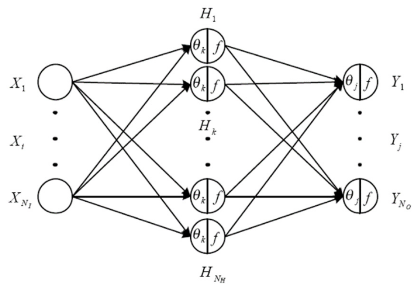
ANNs generally consist of input, output, and procession layers (called hidden layers, as depicted in Figure 1). The basic settings used to construct a BPN are the procession units: the number of hidden layers with the number of nodes at each one.

Figure 1. Illustration of BPN.

Several indicators—usually root-mean-square error (RMSE) and error rate—are used to test the reliability of a network and the validity of its structure. Its learning process is used to adjust network-linking weights by applying the learning algorithm from the input data, as well as the error function, which is adopted to measure the learning effect of the BPN. When the BPN’s leaning process finishes, the minimum error—which represents the maximum predicting accuracy—is expected. Its architecture is shown in Figure 1 [31].

$$Y_j\hspace{0.33em}=\hspace{0.33em}f({\displaystyle {\displaystyle \sum }_i^{}\hspace{0.33em}{W}_{ij}\hspace{0.17em}{X}_i}\hspace{0.17em}-\hspace{0.33em}{\theta }_j)\hspace{0.33em}$$

where:

• Y_j: output data;
• f: transfer function;
• W_ij: weighting of connecting node i to node j;
• X_i: input data;
• θ_j: threshold.

The learning process of a neural network requires the collection of data in advance. Collected samples must be divided into two parts: samples for training and samples for testing. In the network learning phase, learning can be conducted repeatedly until it converges with the network training. In terms of the network test, some indicators may be used as a basis, such as the root-mean-square error (RMSE) and the error rate.

A neural network consists of the above-mentioned input layer, a hidden layer, and an output layer. The learning process is used to adjust the weights of the network links using the learning algorithm from the learning samples. The error function is used to measure the network learning effect. The network learning process is also a process of minimizing the error function, as the smaller the error, the higher the prediction accuracy. Furthermore, the error is generally expected to be minimized as much as possible.

In terms of the BPN, five important parameters must be set: neural network design, learning iterations, learning rate, momentum term, and transfer function. These parameters do not have a clear set of values. Only approximate guidance can be provided, based on the complexity of the issues and the level of noise. The parameters are generally set through trial and error and other data-mining methods. The setting of all parameter values causes a considerable impact on the performance of the network, which is described below.

3.2. TM

The TM, otherwise known as the process robustness study [32] or design of experiment (DOE), in the West, are prevalent in the field of quality engineering and have been shown to be capable of identifying critical factors influencing poor product quality in manufacturing processes. The TM is a low-cost and high-benefit experimental method that provides improvement of product quality through design rather than testing. It allows the design of fewer experimental profiles and conducts experiments using less time and with lower costs to achieve quality optimization. To reduce the number of experiments, an appropriate experiment orthogonal array table based on control factors and the number of levels must be chosen. The objective of the design is to seek optimization and maintain the robustness of the research content by minimizing the effects of the variation of the influencing factors [33].

In particular, the S/N ratio is defined as the ratio of the average value (signal) to the standard deviation (noise). The larger the value, the better the quality. The S/N ratio can be used as a statistical measurement in the Taguchi experiment, and it can also be employed to examine the impact on product quality under different level factors and noise factors. It can be divided into the following three different patterns in terms of different engineering issues: nominal-the-best (NTB), smaller-the-best (STB), and larger-the-best (LTB) [34].

For the NTB, the S/N ratio is $10\times \log \left[\frac{S-V_e}{n\times V_e}\right]$, where $S=\frac{1}{n}\times {\left({\displaystyle \sum }_{i=1}^n{y}_i\right)}^2$, $V_e=\frac{\sum {\left( y_i-\overline{y}\right)}^2}{n-1}$, and $\overline{y}$ is the average for all experiments. The NTB index is applicable to the cases that are expected to obtain certain performance characteristics.

For LTB, the S/N ratio is $-10\times \log \left[\frac{{{\displaystyle \sum }}_{i=1}^n y_i^2}{n}\right]$. The LTB index is for the cases of maximizing the performance characteristics.

For STB, the S/N ratio is $-10\times \log \left[\frac{{{\displaystyle \sum }}_{i=1}^n y_i^2}{n}\right]$. The STB index is suitable for the cases of minimizing the performance characteristics. The STB index is adopted in this study, as the smallest RMSE is the best for the BPN models.

After calculating the S/N ratio for each experiment, each criterion is obtained by taking the average of all the S/Ns within the criterion in accordance with the designed orthogonal array.

The main purpose of the TM is to acquire the best information based on fewer experiments, choose the appropriate orthogonal array table based on the control factors and number of levels, and plan a complete experimental scheme to execute the data from the information obtained. The symbol of an orthogonal array table is generally $L_a\left(b^c\right)$, where L refers to the Latin square; a to the number of experiments; b to the number of levels of control factors; and c to the total number of control factors. The inner product in any two lines in the orthogonal array table is zero, and the average effect between factors reaches an equilibrium state. In the application of the orthogonal array table, experiments were conducted based on the configured profiles in the table; the experiments were performed repeatedly to show objectivity. In the case of uncontrollable interference factors, the combination of two orthogonal array tables was applied to place interference factors in the external table and enhance the accuracy of the experiment. For a more detailed description of TM, please refer to Wu [18].

4. Case Study

In this section, a CVS site selection prediction model is established—based on actual collected data—by applying BPN in accordance with the research architecture and the method described in Section 3. To establish a robust prediction model, the TM is applied to identify the optimal parameters for the execution of the BPN.

4.1. Data Collection

First, the determinate factors for a new chain of convenience stores in this real case included nine input data items: trade area characteristics (A) (A1—residential area and A2—commercial area), competitiveness of other CVSs (B), competitiveness of supermarkets (C), people flow (D), major customer type (E), number of households within a radius of 100 m (F), store location (G), visibility (H), and usable area (I) (as defined in Table 1). We then collected the data of the nine factors from 96 new stores of a well-known CVS chain store in Taiwan (see Table 2).

Table 1. Definitions of site selection assessment indicators.

No	Factor		Definition
A	Customer source	A1	Residential area (dominated by the residential population surrounding the site, with fixed consumption and higher turnover on holidays and non-work-days compared with weekdays)
		A0	Business area (dominated by transient populations surrounding the site engaging in commercial activities in the area, with a higher number of customers on weekdays)
B	Competitiveness of other CVSs		The number of other chain CVSs within a radius of 200 M + self-owned CVSs within a radius of 100 M
C	Competitiveness of supermarkets		The number of supermarkets and other types of retail stores within a radius of 200 M
D	Customer flow		Pedestrian flow through the site + the number of motorcycles passing through the site
E	Major customer type		(1) Workers (2) Students (3) Pedestrian flow (4) Nearby residents
F	The number of households		The number of effective households within a radius of 100M
G	Store location		(1) Intersection of two parkways (between main streets) (2) Intersection of one parkway and byway (between minor streets) (3) Off intersection
H	Visibility		The signboard is visible from 100 m away
I	Usable area		The area of the store (greater than 75 m2 or not)

Table 2. Training network data table.

No	A1	A2	B	C	D	E	F	G	H	I	Predict	No	A1	A2	B	C	D	E	F	G	H	I	Predict
1	1	0	100	60	15.16	100	17.16	80	50	1.1	70,400	49	1	0	100	100	14.58	80	21.32	80	50	1.1	52,790
2	1	0	20	100	14.83	80	30.52	50	100	1.1	60,300	50	1	0	10	20	7.53	100	3.28	80	100	1.1	47,500
3	1	0	65	55	12.83	80	14.44	80	50	1.1	43,040	51	1	0	100	100	13.44	0	5.4	70	100	1.1	60,800
4	1	0	10	100	5.54	100	8.56	80	100	1.1	49,700	52	1	0	20	100	9.13	100	15.48	50	100	1.1	73,200
5	1	0	100	40	0.05	80	2.88	100	100	1.1	65,000	53	1	0	100	100	10.07	100	6.48	80	100	1.1	69,600
6	1	0	100	100	10.30	100	28.92	80	100	1.1	87,200	54	1	0	10	0	11.41	80	13.88	80	100	1.1	33,500
7	0	1	20	100	11.76	80	6.75	80	50	1.1	32,550	55	1	0	65	100	6.30	80	7.96	80	100	1.1	63,000
8	1	0	15	5	12.73	100	3.68	50	100	1.1	34,700	56	1	0	100	50	7.89	80	5.96	50	100	1.1	39,020
9	1	0	100	100	1.54	80	0	100	100	1.1	47,050	57	1	0	20	75	6.84	80	26.88	80	50	1.1	54,600
10	1	0	0	50	5.44	80	4.12	50	0	1.1	32,900	58	1	0	30	100	9.49	100	4.28	50	100	1.1	44,200
11	1	0	100	100	4.06	80	3.12	50	50	1.1	55,000	59	1	0	40	100	12.70	100	7.04	50	50	1.1	39,100
12	1	0	30	100	14.80	80	28.2	80	50	1.1	68,000	60	1	0	60	100	6.69	100	50.08	80	50	1.1	85,200
13	1	0	10	50	6.15	80	32.04	20	50	1.1	33,000	61	1	0	30	75	9.03	100	13.72	50	50	1.1	49,000
14	1	0	100	100	3.21	80	4.16	50	0	1.1	52,600	62	1	0	5	75	5.35	80	19.44	50	100	1.1	43,800
15	1	0	25	100	10.50	100	4.8	50	50	1.1	40,700	63	1	0	10	100	7.10	80	10.8	80	50	1.1	32,520
16	1	0	25	100	24.80	100	27.48	80	100	1.1	49,080	64	1	0	10	100	5.63	80	4.96	80	50	1.1	50,000
17	1	0	10	35	14.48	100	13.44	80	50	1.1	49,000	65	1	0	100	100	6.91	80	20.68	80	50	0.9	46,750
18	1	0	20	60	12.59	100	19.92	80	100	1.1	59,100	66	1	0	10	100	5.48	80	14.28	50	100	1.1	41,500
19	1	0	100	100	11.05	80	17.8	50	50	0.9	50,000	67	1	0	15	100	13.49	100	14.72	100	50	1.1	43,300
20	0	1	10	100	10.08	100	13.25	50	100	1.1	45,000	68	1	0	100	60	10.54	100	6	20	100	1.1	51,100
21	1	0	100	100	6.50	100	13.24	50	100	1.1	61,600	69	1	0	100	100	3.91	100	6.92	80	100	1.1	63,200
22	1	0	10	100	6.06	100	5.24	80	50	1.1	43,800	70	1	0	0	45	6.71	100	10.96	70	50	1.1	38,500
23	1	0	30	75	4.56	0	52.4	80	50	1.1	74,500	71	1	0	20	100	10.17	80	36.96	50	50	1.1	59,100
24	1	0	20	80	2.81	100	2.08	50	100	1.1	42,500	72	1	0	20	100	4.38	100	8.56	80	100	1.1	55,200
25	1	0	10	100	9.20	100	13.48	80	50	1.1	45,100	73	1	0	40	100	4.74	0	15.68	80	50	1.1	45,700
26	1	0	100	100	24.48	100	25.88	80	100	1.1	73,700	74	1	0	20	55	5.51	0	25.76	80	100	1	41,800
27	1	0	30	100	8.80	80	22.56	80	100	1.1	68,400	75	1	0	40	100	8.65	80	23.2	80	50	1.1	63,200
28	1	0	40	55	6.17	80	11	50	100	1.1	44,100	76	1	0	20	100	8.75	80	16.76	50	100	1.1	51,000
29	1	0	20	55	7.43	100	14.32	80	100	1.1	56,100	77	1	0	10	65	9.47	0	42	20	100	1.1	39,500
30	1	0	20	100	2.62	100	10.64	80	100	1.1	51,300	78	1	0	20	100	10.31	80	19.72	80	100	1.1	50,700
31	1	0	100	100	7.24	100	5.44	50	100	1.1	52,100	79	1	0	100	100	6.91	80	22.72	80	0	1.1	64,800
32	1	0	30	100	8.32	80	8.52	50	50	1.1	70,100	80	0	1	25	35	10.27	100	27.95	20	100	1.1	44,500
33	1	0	10	60	3.68	80	3.12	80	50	1.1	40,800	81	1	0	0	100	13.06	80	15.48	50	50	1.1	40,700
34	1	0	10	100	9.82	80	17.64	80	100	1	33,870	82	0	1	20	55	3.35	100	12.4	20	100	1.1	40,000
35	1	0	15	100	20.45	100	1.44	100	100	1.1	64,200	83	1	0	100	100	4.75	0	4.24	80	100	1.1	42,000
36	1	0	15	100	3.86	100	27.8	20	100	1	24,800	84	1	0	15	100	14.95	100	17.16	50	50	1.1	43,600
37	1	0	40	100	4.15	100	7.92	50	100	1.1	44,000	85	1	0	100	100	6.28	80	9.04	50	50	1.1	52,600
38	1	0	100	100	1.21	0	37.08	50	50	1.1	73,600	86	1	0	100	90	13.03	80	15.88	50	100	1.1	45,460
39	1	0	30	100	15.83	80	17.85	80	50	1.1	57,200	87	1	0	15	100	8.33	0	41	80	100	1.1	60,100
40	1	0	40	75	2.52	100	29.6	20	50	1.1	39,100	88	1	0	10	85	6.28	80	1.4	50	100	1.1	34,900
41	1	0	20	100	9.21	100	10	80	100	1.1	43,300	89	1	0	30	100	7.88	100	9.28	100	50	1.1	59,300
42	1	0	100	100	22.02	80	5.84	50	50	1	36,280	90	1	0	40	100	18.76	100	18.72	80	50	1.1	66,300
43	1	0	20	35	12.96	80	4.72	80	50	1.1	48,000	91	1	0	40	50	8.64	80	28.76	80	100	1.1	60,900
44	1	0	10	100	15.92	80	12.72	50	100	1.1	35,600	92	1	0	55	55	8.80	80	17.32	80	50	1.1	62,000
45	1	0	100	100	7.18	80	13.84	50	50	1.1	71,000	93	1	0	30	40	20.87	100	29.6	80	50	1.1	40,100
46	1	0	30	100	9.44	80	16.16	50	100	1.1	46,000	94	1	0	10	100	25.23	80	3.2	80	100	1.1	51,100
47	0	1	20	40	18.97	80	24.12	100	100	1.1	55,000	95	1	0	100	100	7.06	80	39.92	80	100	1.1	96,900
48	1	0	5	10	7.98	100	14.68	80	100	1.1	43,800	96	1	0	100	80	12.81	100	15.88	50	50	1.1	44,320

The existing evaluated model was based on the idea that the initial prediction turnover of a new store is obtained based on the sum of each of the actual data factors of the nine determinants times the given weight of each determinant. Whether a new store is a success is based the actual turnover. If the value of the predicted turnover/average actual turnover per day over an operational period of six months is higher than 90% (0.9), then the new store is defined as a success; otherwise, it is a failure. For instance, the prediction score form of Store 1 is shown in Table 2. The scores for factors B, C, D, E, F, G, and H are 100, 60 × (20 + 35 + 5), 11.7 × (6.6 + 5.1), 100, 17.2, 80 × (30 + 50), and 50 respectively (Table 3), and we can estimate the number of visitors at 914.5—based on the weightings of the residential area (Factor A) (Table 4). Therefore, the predicted turnover/per day is 914.5 × 70 (customer price of residential area) × 1.1 (Factor I: the area of store 1 is greater than 100 square meter) = 70,400. Finally, we can predict the daily turnover of each store and collect the average actual daily turnover for six months from the 96 new stores, as summarized in Table 5.

Table 3. Scores of the factors.

Factors							Base	Score
B: Competitiveness of other CVSs
BQ1	Competitive store category	Major competitive CVS (0)	Minor competitive CVS (20)	Local chain CVS (30)	Self-operated CVS (40)	None (100)	1	100
BQ2	Relative distance	<50 m (0)	50–100 m (5)	100–200 m (10)	>200 m (20)			NA
BQ3	Competitive store proximity	good (0)	acceptable (10)	poor (20)				NA
BQ4	Competition store opening hours	24 h	not 24 h					NA
C: Competitiveness of Supermarkets:
CQ1	Number of stores	≧4 (0)	3 (5)	2 (20)	1 (40)	none (100)		20
CQ2	Relative distance	<50 m (0)	50–100 m (10)	100–200 m (15)	>200 m (35)			35
CQ3	Competition store closed hours	after 22:00 (0)	21:00–22:00 (5)	20:00–21:00 (10)	before 20:00 (15)			5
D: People flow
DQ1	Survey time	07:00–09:00	12:00–14:00	17:00–19:00	21:00–23:00
DQ2	Pedestrian	264					40	264/40 = 6.6
DQ3	Motorcycle	2568					500	2568/500 = 5.1
E: Major customer type
EQ1		Single source (0)	Two sources (80)	>Two sources (100)				100
F: Number of households
FQ2	Number of households	429					25	429/25 = 17.2
G: Store location
GQ1	Store location	Off intersection (0)	Between minor streets (30)	Between main streets (50)				30
GQ2	Width	<6 m (0)	6–10 m (20)	>10 m (50)				50
H: Visibility
HQ1	Visibility	<50 m (0)	50–100 m (50)	>100 m (100)				50
I: Area
IQ1	Usable area	<50 m2 (0.9)	50–100 m2 (1.0)	>100 m2 (1.1)

Table 4. Prediction of the number of visitors.

Factor	Score	Weighting of Residential Area (Factor A)	Sub-Sum
B	100.0	0.29%	288.5
C	60.0	0.06%	34.6
D	11.7	0.67%	79.0
E	100.0	0.08%	76.9
F	17.2	0.58%	99.0
G	80.0	0.38%	307.7
H	50.0	0.06%	28.8
Sum			914.5

Table 5. Difference between predicted daily turnover and actual daily turnover.

Store	Predict.	Actual	Difference	Ratio	Success	Store	Predict	Actual	Difference	Ratio	Success
1	70,400	55,023	15,377	0.78		49	52,790	47,007	5783	0.89
2	60,300	46,923	13,377	0.78		50	47,500	37,819	9681	0.80
3	43,040	39,375	3665	0.91	1	51	60,800	40,152	20,648	0.66
4	49,700	47,214	2486	0.95	1	52	73,200	46,710	26,490	0.64
5	65,000	39,669	25,331	0.61		53	69,600	61,930	7670	0.89
6	87,200	91,004	3804	1.04	1	54	33,500	67,507	34,007	2.02	1
7	32,550	42,914	10,364	1.32	1	55	63,000	64,056	1056	1.02	1
8	34,700	53,743	19,043	1.55	1	56	39,020	36,379	2641	0.93	1
9	47,050	43,513	3537	0.92	1	57	54,600	35,050	19,550	0.64
10	32,900	44,322	11,422	1.35	1	58	44,200	30,780	13,420	0.70
11	55,000	56,081	1081	1.02	1	59	39,100	37,799	1301	0.97	1
12	68,000	48,007	19,993	0.71		60	85,200	46,564	38,636	0.55
13	33,000	35,872	2872	1.09	1	61	49,000	55,184	6184	1.13	1
14	52,600	39,851	12,749	0.76		62	43,800	39,196	4604	0.89
15	40,700	33,121	7579	0.81		63	32,520	70,667	38,147	2.17	1
16	49,080	52,619	3539	1.07	1	64	50,000	42,152	7848	0.84
17	49,000	40,460	8540	0.83		65	46,750	50,033	3283	1.07	1
18	59,100	48,155	10,945	0.81		66	41,500	46,384	4884	1.12	1
19	50,000	53,140	3140	1.06	1	67	43,300	80,205	36,905	1.85	1
20	45,000	53,561	8561	1.19	1	68	51,100	41,517	9583	0.81
21	61,600	33,410	28,190	0.54		69	63,200	40,175	23,025	0.64
22	43,800	44,622	822	1.02	1	70	38,500	43,788	5288	1.14	1
23	74,500	37,861	36,639	0.51		71	59,100	44,298	14,802	0.75
24	42,500	47,955	5455	1.13	1	72	55,200	62,976	7776	1.14	1
25	45,100	43,360	1740	0.96	1	73	45,700	30,051	15,649	0.66
26	73,700	53,278	20,422	0.72		74	41,800	45,711	3911	1.09	1
27	68,400	67,508	892	0.99	1	75	63,200	47,535	15,665	0.75
28	44,100	40,352	3748	0.92	1	76	51,000	36,745	14,255	0.72
29	56,100	42,921	13,179	0.77		77	39,500	48,996	9496	1.24	1
30	51,300	57,308	6008	1.12	1	78	50,700	73,138	22,438	1.44	1
31	52,100	49,883	2217	0.96	1	79	64,800	61,396	3404	0.95	1
32	70,100	50,055	20,045	0.71		80	44,500	20,763	23,737	0.47
33	40,800	51,543	10,743	1.26	1	81	40,700	43,101	2401	1.06	1
34	33,870	52,791	18,921	1.56	1	82	40,000	58,015	18,015	1.45	1
35	64,200	42,554	21,646	0.66		83	42,000	51,495	9495	1.23	1
36	24,800	51,127	26,327	2.06	1	84	43,600	48,268	4668	1.11	1
37	44,000	50,130	6130	1.14	1	85	52,600	56,032	3432	1.07	1
38	73,600	44,734	28,866	0.61		86	45,460	45,805	345	1.01	1
39	57,200	48,733	8467	0.85		87	60,100	52,036	8064	0.87
40	39,100	56,205	17,105	1.44	1	88	34,900	37,717	2817	1.08	1
41	43,300	38,257	5043	0.88		89	59,300	51,201	8099	0.86
42	36,280	45,635	9355	1.26	1	90	66,300	39,763	26,537	0.60
43	48,000	43,643	4357	0.91	1	91	60,900	65,757	4857	1.08	1
44	35,600	22,774	12,826	0.64		92	62,000	45,233	16,767	0.73
45	71,000	47,499	23,501	0.67		93	40,100	44,463	4363	1.11	1
46	46,000	40,230	5770	0.87		94	51,100	55,101	−4001	1.08	1
47	55,000	74,899	19,899	1.36	1	95	96,900	52,973	43,927	0.55
48	43,800	50,339	6539	1.15	1	96	44,320	39,231	5089	0.89
						RMSE		15,791		Success	53
						MAE		12,155		Success rate	55%
						MSE		249,363,237

As shown in Table 5, the average actual daily turnover per month over six months in Store 1 is 55,023, and the ratio of the predicted daily turnover/average actual daily turnover is 0.78. If this value is smaller than 0.9, then the new store is defined as a failure. As depicted, the average difference between the actual daily turnover and the predicted daily turnover was $NTD 12,061/per store and the RMSE reached $NTD 10,188. A total of 53 stores were successful (defined as the predicted turnover/actual turnover is higher than 0.9), and the success rate (or prediction accuracy rate) was 55% (as shown in Table 5). This study used a BPN network to validate whether further reducing the error and improving the prediction accuracy rate for a new store would be possible. The major differences between the predicted and actual turnovers can be attributed to one major set of reasons. Based on one of the managers involved in the site selection decision in this CVS company, the store personnel’s operating stabilities, the store’s management style, and the inventory principles essentially contributed to the turnover of their CVSs. However, at the time of data analysis, such variation was not yet recognized in the data sources for the CVS site selection. This issue is discussed in the last section of this paper.

4.2. Neural Network Parameter Design

BPN networks are nonlinear models. Therefore, algorithm mode was used to approach the best linked weighted value and the bias value by means of performing iterations. In the experiment, a computer program was developed using a Qnet BPN with 10 types of input data: residential area (X₁), commercial area (X₂), competitiveness of CVSs (X₃), competitiveness of supermarkets (X₄), people flow (X₅), major customer type (X₆), number of households within a radius of 100 m (X₇), store location (X₈), visibility (X₉), and usable area (X₁₀). The output data were the actual daily turnover (Y₁). The five most important factors influencing the BPN network design were (A); learning iterations (B); learning rate (C); momentum term (D); and transfer function (E). In terms of the prediction result of the BPN network, the smaller the error, the better the result. Therefore, the smaller-the-better (STB) of the S/N ratio of TM was used. In the TM, an orthogonal array table of ${\mathrm{L}}_{16}\left(4^5\right)$ (as in Table 6) was chosen, and the above five control factors were placed into Table 6 to shorten the time for the experiment.

Table 6. L₁₆(4⁵) Orthogonal Array.

Experiment	A	B	C	D	E
1	1	1	1	1	1
2	1	2	2	2	2
3	1	3	3	3	3
4	1	4	4	4	4
5	2	1	2	3	4
6	2	2	1	4	3
7	2	3	4	1	2
8	2	4	3	2	1
9	3	1	3	4	2
10	3	2	4	3	1
11	3	3	1	2	4
12	3	4	2	1	3
13	4	1	4	2	3
14	4	2	3	1	4
15	4	3	2	4	1
16	4	4	1	3	2

Because there was no defined method for setting the parameters of the neural network, the distribution principles of the levels of factors were as follows:

• Neural network design (number of units in the hidden layer)

Based on the specified principle, the number of first hidden nodes was designed by applying the method of averaging (number of units in the input layer + the number of units in the output layer)/2, the method of summation (the number of units in the input layer + the number of units in the output layer), and the number of second hidden nodes, designed by applying a radical of the number of input layers × the number of output layers.

2.

Learning iterations

Based on general principles, 1000; 3000; 6000; 10,000; and other intervals were set as the average value.

3.

Learning rate and momentum term

The learning rate and the momentum term would affect the correction of the weighted value of the network and cause adverse effects on the convergence effect of the network if they were too big or too small. Based on the experience values, the learning rate was set between 0.1 and 1. Values with equal intervals, such as 0.1, 0.4, 0.7, and 0.9, were adopted in this research.

4.

Transfer function

The transfer function was designed based on the four functions provided in the Qnet97 for Window Software (Version 1.0).

The distribution of the levels of the factors is shown in Table 7.

Table 7. Distribution list of the levels of factors of the neural network.

	Factor	Neural Network Design (A)	Learning Iteration (B)	Learning Rate (C)	Momentum Term (D)	Transfer Function (E)
Level
Level 1		Five nodes, one hidden layer	1000	0.1	0.1	Sigmoid
Level 2		Ten nodes, one hidden layer	3000	0.4	0.4	Gaussian
Level 3		Five nodes in the first hidden layer; three nodes in the second hidden layer	6000	0.7	0.7	Hyperbolic Tangent
Level 4		Ten nodes in the first hidden layer; three nodes in the second hidden layer	10,000	0.9	0.9	Hyperbolic Secant

4.3. TM Analytical Results

In this study, the “bigger-the-best” characteristic was employed, as the MD between the normal and abnormal groups was the “larger-the-better” in order to be significantly distinguished. For each test, followed by the factor setting in the orthogonal array (as in Table 6), an S/N ratio was obtained (listed in Table 8). The factorial effect of each factor was hence calculated and shown in Table 9. A total of three folders were created, and three sets of data were used to calculate the S/N (signal-to-noise ratio) value. The root-mean-square error (RMSE) of the results of each experiment was calculated using the RMSE of the test set; ten-folder cross validation for the ANN was then used repeatedly to calculate the S/N. In total, 16 experiments were conducted, as shown in Table 8, to respectively record the errors of the simulation results for the BPN network. The RMSE of the test data was used to obtain the average value of the error, and the S/N ratio in each experiment was obtained based on the STB characteristic (see Table 8).

Table 8. Experiment error data.

Exp.	Fold 1	Fold 2	Fold 3	Average	St dev	S/N
1	0.122132	0.130395	0.123223	0.12525	0.004489	23.2695
2	0.147806	0.147416	0.148411	0.147878	0.000501	21.8307
3	0.114294	0.130201	0.114288	0.119594	0.009186	23.6575
4	0.114294	0.431601	0.409061	0.318319	0.17705	14.3572
5	0.409061	0.431601	0.409061	0.416574	0.013013	12.8321
6	0.166123	0.206958	0.173732	0.182271	0.021715	19.9735
7	0.186692	0.20525	0.197209	0.196384	0.009306	19.3602
8	0.167459	0.19631	0.166127	0.176632	0.017055	20.2605
9	0.114294	0.130202	0.1142	0.119565	0.009212	23.6565
10	0.147329	0.16983	0.114294	0.143818	0.027934	21.9647
11	0.161272	0.219702	0.159119	0.180031	0.034373	20.0176
12	0.158788	0.178615	0.180458	0.17262	0.012015	20.4729
13	0.114289	0.130207	0.114303	0.1196	0.009186	23.6571
14	0.212842	0.162019	0.12926	0.16804	0.042115	20.5424
15	0.226479	0.172241	0.202408	0.200376	0.027176	19.1389
16	0.231873	0.180894	0.188176	0.200314	0.027572	19.14

Table 9. S/N ratio factor response list.

	Neural Network Design	Learning Iteration	Learning Rate	Momentum Term	Transfer Function
1	20.77873798	20.85457474	20.60016135	20.91125083	21.15840307
2	18.10658004	21.07781527	18.56867528	21.44147353	20.99761299
3	21.52867521	20.54355308	22.0299774	19.39858585	21.94028713
4	20.61961943	18.55766957	19.83479863	19.28230244	16.93730947
Effect	3.422095173	2.520145701	3.461302121	2.159171086	5.002977668
Rank	3	4	2	5	1
Best level	A3	B2	C3	D2	E3

According to Table 8, the highest S/N ratio (23.6575) was observed in the third experiment and involved factors A1, B3, C3, D3, and E3. However, from the S/N ratio factor response list (Table 9), the transfer function was mostly affected by effect and rank factors and levels, followed by the learning rate.

As shown in Table 9, the optimal parameter combination consisted of A3, B2, C3, D2, and E3. According to the combination of A3, B2, C3, D2, and E3, we split the training network data in Table 5 into three sets in the order 1–25, 26–50, 51–75, and carried out the optimal combination of BPN three times. The S/N ratio was 16.2946 and the 95% confidence interval was calculated as 14.253997–18.415372, which was confirmed to be within the confidence interval. The data are shown in Table 10.

Table 10. The results of experience of optimal parameters.

Experiment	Fold 1	Fold 2	Fold 3	S/N	Upper Bond	Lower Bond
Training 1–25	0.259155	0.13692	0.318543	14.2625
Training 26–50	0.125047	0.165635	0.201135	17.7714	18.415372	14.253997
Training 51–75	0.24473	0.143677	0.141125	16.9701
Retesting 76–96	0.15075	0.197292	0.236022	16.2946

Therefore, to verify the combination of the optimal parameters, we utilized the two combinations to obtain the S/N ratio (see Table 11). As shown in Table 11, we found that the combination of A3, B2, C3, D2, and E3 had a larger S/N ratio.

Table 11. S/N ratio of reverification.

Experiment	Fold 1	Fold 2	Fold 3	Average	St. Dev	S/N
Combination of A3:B2:C3:D2:E3	0.15075	0.197292	0.236022	0.194688	0.042696	19.3049
Combination of A1:B3:C3:D3:E3	0.257151	0.242185	0.203655	0.23433	0.027599	17.7922

Therefore, the optimal parameter combination consisted of A3, B2, C3, D2, and E3, respectively, including the neural network design (five nodes in the first hidden layer and three nodes in the second hidden layer), learning iterations (3000), learning rate (0.7), momentum term (0.4), and transfer function (hyperbolic tangent), respectively. Based on the above optimal parameter design result of the BPN, the network architecture was, therefore, designed (see Figure 2).

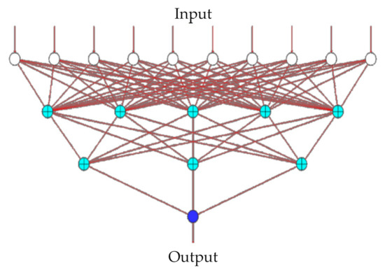
Figure 2. Network design architecture diagram.

4.4. Experimental Results and Validation

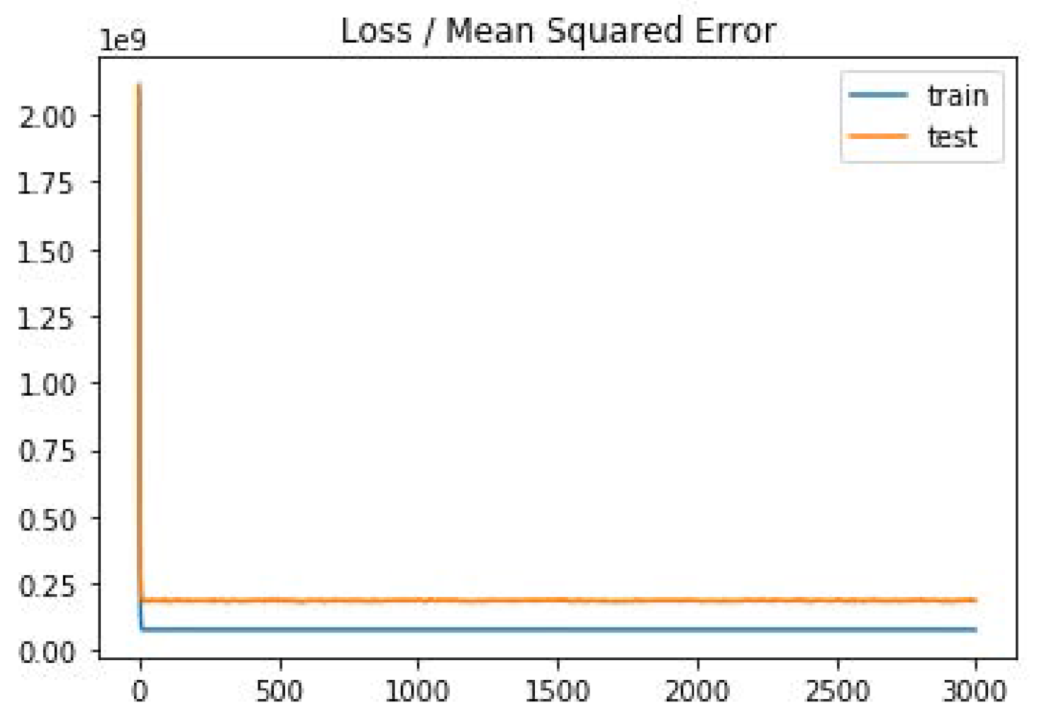
This research obtained the weights and deltas from the BPN Software (Qnet97 for Window, Version 1.0) according to the above-mentioned best parameter conditions and training and imported 96 sets of data for validation. It then deduced the results, as shown in Figure 3 and Table 12. As shown in Figure 3, the MSE became stable with reasonable convergence, so there was no over-fitting problem. As shown in Table 12, the RMSE, MAE, and MSE of the 96 sets of data obtained and validated with optimized weighted values and biases were reduced to 9810, 7750, and 96,229,425, respectively. Compared with the RMSE (15,791), MAE (12,155), and MSE (249,363,237) of the original data, the error rate was reduced by 38% (RMSE), 36% (MAE), and 61% (MSE), respectively. A total of 62 stores was thus successful in the prediction, resulting in an accuracy rate of up to 65%. Compared with the accuracy rate (55%) of the original data, the accuracy rate increased by 18.2%. Therefore, the results indicated that the proposed prediction model had a higher success rate and lower RMES value; the proposed prediction model therefore provides a valuable reference for the industry. In summary, we found that the chances of success in establishing a new store were improved through the analysis of the objective data using the store site selection prediction model established in this research.

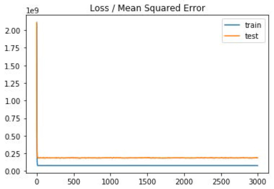
Figure 3. Mean squared error. (Note: le9 = 1 × 10⁹).

Table 12. Actual deduction results.

Store	Target	Prediction	Error Value	Prediction Rate	Accuracy	Store	Target	Prediction	Error Value	Prediction Rate	Accuracy
1	55,023	45,854	9169	1.20	1	49	47,007	49,091	2084	0.96	1
2	46,923	49,244	2321	0.95	1	50	37,819	45,503	7684	0.83
3	39,375	45,845	6470	0.86		51	40,152	45,367	5215	0.89
4	47,214	58,166	10,952	0.81		52	46,710	47,061	351	0.99	1
5	39,669	58,107	18,438	0.68		53	61,930	46,147	15,783	1.34	1
6	91,004	87,454	3550	1.04	1	54	67,507	45,464	22,043	1.48	1
7	42,914	57,043	14,129	0.75		55	64,056	46,985	17,071	1.36	1
8	53,743	46,913	6830	1.15	1	56	36,379	45,538	9159	0.80
9	43,513	58,137	14,624	0.75		57	35,050	43,322	8272	0.81
10	44,322	41,168	3154	1.08	1	58	30,780	45,571	14,791	0.68
11	56,081	52,364	3717	1.07	1	59	37,799	45,458	7659	0.83
12	48,007	45,539	2468	1.05	1	60	46,564	48,266	1702	0.96	1
13	35,872	41,905	6033	0.86		61	55,184	45,607	9577	1.21	1
14	39,851	51,025	11,174	0.78		62	39,196	47,428	8232	0.83
15	33,121	42,860	9739	0.77		63	70,667	46,256	24,411	1.53	1
16	52,619	56,793	4174	0.93	1	64	42,152	45,659	3507	0.92	1
17	40,460	47,130	6670	0.86		65	50,033	50,749	716	0.99	1
18	48,155	55,865	7710	0.86		66	46,384	46,644	260	0.99	1
19	53,140	41,386	11,754	1.28	1	67	80,205	51,606	28,599	1.55	1
20	53,561	57,164	3603	0.94	1	68	41,517	45,511	3994	0.91	1
21	33,410	51,917	18,507	0.64		69	40,175	47,094	6919	0.85
22	44,622	57,347	12,725	0.78		70	43,788	45,564	1776	0.96	1
23	37,861	45,750	7889	0.83		71	44,298	52,693	8395	0.84
24	47,955	46,572	1383	1.03	1	72	62,976	49,760	13,216	1.27	1
25	43,360	54,439	11,079	0.80		73	30,051	45,444	15,393	0.66
26	53,278	48,830	4448	1.09	1	74	45,711	45,511	200	1.00	1
27	67,508	55,690	11,818	1.21	1	75	47,535	65,842	18,307	0.72
28	40,352	41,985	1633	0.96	1	76	36,745	46,789	10,044	0.79
29	42,921	56,473	13,552	0.76		77	48,996	45,413	3583	1.08	1
30	57,308	58,213	905	0.98	1	78	73,138	60,417	12,721	1.21	1
31	49,883	53,856	3973	0.93	1	79	61,396	52,210	9186	1.18	1
32	50,055	42,082	7973	1.19	1	80	20,763	27,751	6988	0.75
33	51,543	53,754	2211	0.96	1	81	43,101	45,484	2383	0.95	1
34	52,791	54,859	2068	0.96	1	82	58,015	46,198	11,817	1.26	1
35	42,554	58,567	16,013	0.73		83	51,495	45,388	6107	1.13	1
36	51,127	41,989	9138	1.22	1	84	48,268	45,612	2656	1.06	1
37	50,130	48,448	1682	1.03	1	85	56,032	45,605	10,427	1.23	1
38	44,734	39,971	4763	1.12	1	86	45,805	45,853	48	1.00	1
39	48,733	45,646	3087	1.07	1	87	52,036	45,553	6483	1.14	1
40	56,205	42,024	14,181	1.34	1	88	37,717	45,467	7750	0.83
41	38,257	57,763	19,506	0.66		89	51,201	50,338	863	1.02	1
42	45,635	41,986	3649	1.09	1	90	39,763	46,545	6782	0.85
43	43,643	44,194	551	0.99	1	91	65,757	65,938	181	1.00	1
44	22,774	37,175	14,401	0.61		92	45,233	47,671	2438	0.95	1
45	47,499	45,448	2051	1.05	1	93	44,463	46,158	1695	0.96	1
46	40,230	43,343	3113	0.93	1	94	55,101	45,378	9723	1.21	1
47	74,899	58,563	16,336	1.28	1	95	52,973	49,800	3173	1.06	1
48	50,339	56,292	5953	0.89		96	39,231	41,638	2407	0.94	1
						RMSE		9810		Success	62
						MAE		7750		Success rate	65%
						MSE		96,229,425

4.5. Robustness Evaluation

To evaluate the robustness of the proposed method, different numbers of training instances were used to assess the performance of the ANN-TM prediction models. The results were evaluated based on four considered numbers of training examples: 16, 32, 48, and 64, respectively. Table 13 summarizes the “success rate” for the prediction data of the ANN-TM method. As shown in the table, when there were more training samples, the success rate increased. However, the increase in the success rate gradually decreased.

Table 13. Robustness evaluation.

Number of Training Instances	Success Rate
16	65%
32	69%
48	72%
64	73%

5. Conclusions

The structure of the parameters of a neural network determines the network’s predictive reliability and validity. This study employed a robust experimental design, the TM, to BPN training to efficiently derive the optimal CVS site-selection decision model for the case company. Site-selection methods developed solely using an ANN methodology require time- and cost-intensive effort. In this study, combined with the TM’s experimental design and the S/N ratios to evaluate performance, the BPN decision model confirmed that valid results can be obtained with fewer experiments. The TM can reduce the number of times required for the determination of the BPN for improved convergence and fewer network errors. We assert that with systematic assessment, site selection for a new chain of CVSs can be performed with reduced human bias. The actual operational data of a well-known chain of CVSs was used here to validate the site selection prediction model built in this paper. The results indicated that the predicted accuracy rate and the decision quality of the proposed prediction model were higher than those obtained from the existing decision method of using experienced managers.

The combined application of ANN and TM to a retail business in this study represented a pilot in both the TM application and site selection literature. This study adopted the TM to identify important criteria for the BPN site selection prediction model. By using data from a well-known Taiwanese CVS chain, we provided a valuable and practical alternative and thus contributed knowledge about chain CVS site-selection decision-making. The deviation of the case company’s actual sales from its sales forecast implied an unsuccessful site selection decision. For chain corporations in Taiwan, site selection criteria are usually employed using similar principles for each criterion—such as types of patron, business area, and location environment. Since the advent of analytical techniques, Taiwanese retailers have tended to apply contemporary advanced data analysis methodologies in their practices; ANNs, for example, are popular. However, with limited knowledge regarding such analytic solutions and a keen desire to achieve efficiency and effectiveness in retail businesses, this study proposed an approach that can enable Taiwanese chain CVSs to appropriately solve site-selection problems.

The managerial implication of applying retail site selection studies is that companies should make efforts to review the feasibility and applicability of the requisite factors for building ANN prediction models. This study demonstrated this in the case company. It is necessary to debrief and re-examine current CVS site location evaluation procedures, including the effective criteria and their scales, based on the predictive accuracy of the ANN procedure. Nonetheless, the definition of successful and unsuccessful CVSs is not unique within the case company. Generally, a successful CVS is defined as one that achieves its revenue and/or other goals. Some unsuccessful CVSs may be considered successes when their actual sales are much higher than the original forecast. Hence, classifying successful and unsuccessful retail stores for BPN analysis is crucial. The approach presented in this study assists in building a systematic design of the BPN predictive model to reduce the cost, time, and personnel involved in the site selection process. The purpose of this study was not to determine the “definite” predictive model for CVS site selection across all CVSs. Other criteria may be more salient in site selection in other business areas or cities.

In addition, as shown in Table 5, there were major differences between the actual turnover and the predictions. This demonstrates the limitation that the source data were collected or encoded by subjective judgements, as the data fields were still treated as important and indicative of store site-location determinants. For future work, this study can be extended by using other prediction tools to build the prediction model to observe the difference. Furthermore, this study was based on one chain CVS in Taiwan; different chain CVSs might have different prediction models. Therefore, this study can be extended by using data from various sources: big data, direct customer behaviors from the Internet of Things (e.g., actual traffic, types of patron, customer travel routes within stores), indirect customer behaviors (e.g., responses on social media, customer mobile behaviors via apps), and store operations (e.g., store personnel working mode, management style, stocking strategy).

References

- Lee, W.I. The Use of Analytical Network Process (ANP) in Selecting the Location of Convenience Stores. Master’s Thesis, National Chin-Yi University of Technology, Taichung, Taiwan, 2011. [Google Scholar]
- Chou, S.P. Analysis of Chinese Restaurant Location in Taipei Urban Area. Master’s Thesis, National Taipei University of Technology, Taipei, Taiwan, 2011. [Google Scholar]
- Erbıyık, H.; Özcan, S.; Karaboğa, K. Retail Store Location Selection Problem with Multiple Analytical Hierarchy Process of Decision Making an Application in Turkey. Procedia-Soc. Behav. Sci. 2012, 58, 1405–1414. [Google Scholar] [CrossRef] [Green Version]
- Roig-Tierno, N.; Baviera-Puig, A.; Buitrago-Vera, J.; Mas-Verdu, F. The retail site location decision process using GIS and the analytical hierarchy process. Appl. Geogr. 2013, 40, 191–198. [Google Scholar] [CrossRef]
- Hernández, T.; Bennison, D. The art and science of retail location decisions. Int. J. Retail Distrib. Manag. 2000, 28, 357–367. [Google Scholar] [CrossRef]
- Kuo, R.J.; Chi, S.C.; Kao, S.S. A decision support system for selecting convenience store location through integration of fuzzy AHP and artificial neural network. Comput. Ind. 2002, 47, 199–214. [Google Scholar] [CrossRef]
- Pokonieczny, K. Using artificial neural networks to determine the location of wind farms: Miedzna district case study. J. Water Land Dev. 2016, 30, 101–111. [Google Scholar] [CrossRef]
- Abujayyab, S.K.M.; Ahamad, M.S.S.; Yahyac, A.S.; Saad, A.M.H.Y. A new framework for geospatial site selection using artificial neural networks as decision rule: A case study on landfill sites. In Proceedings of the Joint International Geoinformation Conference, Kuala Lumpur, Malaysia, 28–30 October 2015; pp. 28–30. [Google Scholar]
- Fallah, M.; Vagharfard, H.; Farajzadeh, M.; Kheslat, N. Assessment of Spatial multi-criteria decision-making with process of the artificial neural networks Method to Site Selection of the Wastewater Treatment Plant (Case study: Qeshm Island). Int. J. Adv. Biol. Biomed. Res. 2014, 2, 2061–2066. [Google Scholar]
- Satman, M.H.; Altunbey, M. Selecting Location of Retail Stores Using Artificial Neural Networks and Google Places API. Int. J. Stat. Probab. 2014, 3, 67–77. [Google Scholar] [CrossRef]
- Khaw, J.F.C.; Lim, B.S.; Lim, L.E.N. Optimal design of neural networks using the Taguchi method. Neurocomputing 1995, 7, 225–245. [Google Scholar] [CrossRef]
- Rajiv, P.D.; Grünhagen, M. International franchising research: Some thoughts on the what, where, when, and how. J. Mark. Channels 2014, 21, 124–132. [Google Scholar]
- Teller, C.; Reutterer, T. The evolving concept of retail attractiveness: What makes retail agglomerations attractive when customers shop at them? J. Retail. Consum. Serv. 2008, 15, 127–143. [Google Scholar] [CrossRef] [Green Version]
- Widaningrum, D.L. A GIS-based approach for Catchment area analysis of convenience store. Procedia Comput. Sci. 2015, 72, 511–518. [Google Scholar] [CrossRef] [Green Version]
- Kaufmann, P.J.; Donthu, N.; Brooks, C.M. Multi-unit retail site selection processes: Incorporating opening delays and unidentified competition. J. Retail. 2000, 76, 113–127. [Google Scholar] [CrossRef]
- Goodchild, M.F. ILACS: A location-allocation model for retail site selection. J. Retail. 1984, 60, 84–100. [Google Scholar]
- Ganesha, H.R.; Aithal, P.S.; Kirubadevi, P. Ideal store locations for Indian retailers—An empirical study. Int. J. Manag. Technol. Soc. Sci. 2002, 5, 215–226. [Google Scholar] [CrossRef]
- Ahedo, V.; Santos, J.I.; Galán, J.M. Knowledge transfer in commercial feature extraction for the retail store location problem. IEEE Access 2021, 9, 132967–132979. [Google Scholar] [CrossRef]
- Aversa, J.; Doherty, S.; Hernandez, T. Big data analytics: The new boundaries of retail location decision making. Appl. Geogr. 2018, 4, 390–408. [Google Scholar] [CrossRef]
- Lin, G.; Chen, X.; Liang, Y. The location of retail stores and street centrality in Guangzhou, China. Appl. Geogr. 2018, 100, 12–20. [Google Scholar] [CrossRef]
- Rohani, A.M.B.M.; Chua, F.-F. Location analytics for optimal business retail site selection. In Proceedings of the Computational Science and Its Applications, ICCSA 2018, Melbourne, VIC, Australia, 2–5 July 2018. [Google Scholar] [CrossRef]
- Mendes, A.B.; Themido, I.H. Multi-outlet retail site location assessment. Int. Trans. Oper. Res. 2004, 11, 1–18. [Google Scholar] [CrossRef] [Green Version]
- Lin, Z.X.; Wang, M.Y.; Wang, Q.B. Retail Management; Wu Nan Publishing Co., Ltd.: Taipei, Taiwan, 2009. [Google Scholar]
- Li, L. Data visualization and retrieval based convenience store location model of fresh products. J. Digit. Inf. Manag. 2017, 15, 125–134. [Google Scholar]
- Achabal, D.D.; Gorr, W.L.; Mahajan, V. MULTILOC: A multiple store location decision model. J. Retail. 1982, 58, 5–25. [Google Scholar]
- Johnston, R.J.; Kissling, C.C. Establishment use patterns within central places. Aust. Geogr. Stud. 1971, 9, 116–132. [Google Scholar] [CrossRef]
- McArthur, E.; Weaven, S.; Dant, R. The evolution of retailing: A meta review of the literature. J. Macromark. 2016, 36, 272–286. [Google Scholar] [CrossRef] [Green Version]
- Applebaum, W. The analog method for estimating potential store sales. In Guild to Store Location Research; Kornblau, Ed.; Addison-Wesley: Boston, MA, USA, 1968. [Google Scholar]
- Chen, K.; Kuang, C.; Wang, L.; Chen, K.; Han, X.; Fan, J. Storm Surge Prediction Based on Long Short-Term Memory Neural Network. Appl. Sci. 2022, 12, 181. [Google Scholar] [CrossRef]
- Yang, X.; Chen, Y.; Teng, S.; Chen, G. Method for Predicting Local Site Amplification Factors Using 1-D Convolutional Neural Networks. Appl. Sci. 2021, 11, 11650. [Google Scholar] [CrossRef]
- Yeh, Y.C. Neural Network Mode Application and Implementation; Scholars Books Co., Ltd.: Taipei, Taiwan, 2009. [Google Scholar]
- Montgomery, D.C. Design and Analysis of Experiments, 6th ed.; John Wiley & Sons, Inc.: Hoboken, NJ, USA, 2005. [Google Scholar]
- Thakur, A.G.; Rao, T.E.; Mukhedkar, M.S.; Nandedkar, V.M. Application of Taguchi Method for Resistance Spot Welding of Galvanized Steel. J. Eng. Appl. Sci. 2010, 5, 22–26. [Google Scholar]
- Taguchi, G.; Chowdhury, S.; Wu, Y. Taguchi’s Quality Engineering Handbook; John Wiley & Sons: Hoboken, NJ, USA, 2005. [Google Scholar]
Publisher’s Note: MDPI stays neutral with regard to jurisdictional claims in published maps and institutional affiliations. |
© 2022 by the authors. Licensee MDPI, Basel, Switzerland. This article is an open access article distributed under the terms and conditions of the Creative Commons Attribution (CC BY) license (https://creativecommons.org/licenses/by/4.0/).