Three-Dimensional Inversion of Semi-Airborne Transient Electromagnetic Data Based on a Particle Swarm Optimization-Gradient Descent Algorithm

Abstract

Semi-airborne transient electromagnetics (SATEM) is a geophysical survey tool known for its ability to perform three-dimensional (3D) observations and collect high-density data in large volumes. However, SATEM data processing is presently restricted to 3D model-driven inversion, which is not conducive to detailed surveys. This paper presents a new 3D model- and data-driven inversion algorithm using the particle swarm optimization (PSO) and gradient descent (GD) algorithms. PSO is used to suppress the multiplicity of solutions associated with inverse problems, and the GD algorithm is employed to accelerate the convergence of the inversion process. For the PSO-GD algorithm, a new model-updating equation is established and a cosine probability function is introduced as a weighting term for PSO and GD algorithms to ensure a smooth transition between the two algorithms in the iterative process. The α-trimmed filter function is used as a regularization constraint to smooth the model. The stability and reliability of the PSO-GD algorithm are verified through numerical simulations. Finally, the new algorithm is applied to the processing of SATEM measurements of the Qinshui coal mine in Jincheng, Shanxi Province, China.

1. Introduction

As an important geophysical survey tool widely applied in many fields (e.g., surveys of geological structures, prospecting of mineral resources, and hydrogeological surveys of coal fields) [1,2,3,4,5,6,7], semi-airborne transient electromagnetics (SATEM) has advantages, such as high efficiency, large data, and high-field adaptability [8,9,10]. Inversion is a key step in geophysical data processing. Currently, SATEM data are mostly inverted using 1D or quasi-2D inversion [2,3,11,12,13,14]. The Earth is constantly suffering from faults, intrusions, and erosive processes that produce a subsurface morphology, which makes the geological structure generally complex. Therefore, it is necessary to perform a 3D inversion interpretation. Three-dimensional inversion of airborne electromagnetic data has attracted more and more attention. A flexible inversion framework was constructed, the lithology and drilling information was added to the inversion, and the multi-parameter inversion was achieved [15,16,17,18]. The above-mentioned inversion is restricted to deterministic algorithms. This paper analyzes the existing algorithms and proposes a hybrid algorithm.

Based on the driving strategy, inversion methods can be approximately categorized into two groups. One group consists of conventional, model-driven inversion methods: the deterministic inversion algorithm, which mainly includes the gradient descent (GD) algorithm [19,20]; the conjugate gradient algorithm [21,22]; and the quasi-Newton method [23,24]. All of these methods use the first- and second-order gradient directions or conjugate direction of the objective function as guidance to correct the model parameters, and these above algorithms have the characteristics of mature theories and high convergence rates. Deterministic inversion algorithms play an important role in 3D geophysical inversion [15,16,17,18]. However, model-driven methods have notable deficiencies in two areas. On the one hand, the inversion result heavily relies on the selection of an initial model [25]. Consequently, these methods are susceptible to falling into certain local optimum solutions near the initial model and face difficulties in converging with global optimum solutions for nonlinear, ill-conditioned geophysical inverse problems [26]. On the other hand, the inversion result lacks an evaluation of the model parameters. These limitations have called into question the accuracy of model-driven inversion methods [27].

The other group is composed of data-driven inversion methods based on statistics or the theory of swarm evolution. Stochastic algorithms include the particle swarm optimization (PSO) algorithm, the simulated annealing algorithm, the genetic algorithm, the bee colony algorithm, neural networks, and the Bayesian algorithm, et cetera [28,29,30,31,32,33,34,35,36,37,38,39]. Using multiple models, stochastic algorithms can not only obtain the better-fitting model, but also estimate the uncertainty of the retrieved solution. Compared to model-driven inversion methods, data-driven inversion methods are more capable of escaping from local optimum solutions, can provide an uncertainty evaluation of the global convergence and inversion result independent of the initial model, and are particularly suitable for solving geophysical inverse problems without a priori information. However, data-driven inversion is often more computationally expansive than model-driven inversion by several orders of magnitude [40]. In recent years, the development of computer science has allowed for an increasing application of data-driven inversion methods for geophysical inverse problems.

PSO is a typical data-driven inversion algorithm inspired by the optimization process involved in the search for food by bird or fish swarms in nature. Compared to other data-driven inversion algorithms, PSO requires fewer models and quickly converges during the optimization process; therefore, it has been extensively applied in many engineering fields. For the first time, Fernández-Álvarez et al. (2006) introduced PSO to the interpretation of geophysical inversion results. They employed this algorithm to interpret the inversion of electrical sounding data [41]. Later, many researchers began to study the application of PSO to geophysical inverse problems. Researchers have introduced PSO to many geophysical fields, such as magnetic techniques, seismology, and gravity, as well as demonstrated its versatility. Researchers have also systematically examined the relationships between the parameters (e.g., the inertia coefficient, as well as the individual and social acceleration coefficients) of the PSO algorithm and improved its convergence rate for geophysical inverse problems, thereby laying a foundation for higher-dimensional inversion [42,43,44,45]. By constraining the objective function with a k-means clustering model, Liu et al. (2018) identified particle swarms from multiple magnetic sources in the presence of complex magnetic anomalies [46]. Pace et al. (2019) successfully inverted two-dimensional magnetotelluric data using a hierarchical PSO algorithm with time-varying acceleration coefficients (HPSO-TVAC) [40]. However, PSO has yet to be applied in 3D electromagnetic (EM) inversion, which is mainly because the high complexity of the 3D models of the EM method restricts the convergence rate of PSO. In particular, the decrease in the modified step size and convergence rate of PSO near an optimum solution renders it susceptible to premature convergence. In addition, the increase in the number of parameters amplifies the problem of over stochasticity associated with PSO and consequently reduces the continuity of the model information in the inversion result, which necessitates the smoothing of the model [26,46].

Through a comprehensive consideration of the advantages and disadvantages of model- and data-driven inversion algorithms, a new 3D inversion algorithm, referred to as the PSO-GD algorithm, was developed for SATEM in this study. In this algorithm, PSO is first used to fit the inversion to ensure global convergence, and then the GD algorithm is employed to accelerate the process of fitting the inversion. A cosine probability function is used as a weighting function for the model-updating equation in the new algorithm to ensure a smooth transition from global to accelerated convergence. The α-trimmed filter function is selected as a regularization constraint for the new algorithm. The model is smoothed to suppress the problem of over stochasticity associated with the 3D PSO-based inversion process. The rest of this paper is organized as follows: First, the basic principle and implementation of the PSO-GD algorithm are presented. Then, the stability and reliability of this algorithm are evaluated based on numerically simulated data. Finally, the PSO-GD algorithm is applied to the 3D inversion of real-world measurements, and conclusions and suggestions on further improving the algorithm are given.

2. Theory and Method

2.1. Forward Simulation Theory

In the inversion process, forward simulation is a crucial factor affecting computational efficiency. In particular, 3D forward simulation of a complex model is generally extremely time consuming and requires high computational power. Therefore, through comprehensive consideration of two aspects of 3D forward simulation, namely, its adaptability in modeling complexity and computational efficiency, 3D forward simulation is performed in this study using the staggered mimetic finite volume approach [47,48].

We begin with Maxwell’s equations of time-varying electromagnetic fields. In forward simulation theory, Maxwell’s equations can be written as follows:

$$\nabla \times E+\mu \frac{\partial H}{\partial t}=0$$

(1)

$$\nabla \times H-\sigma E-\epsilon \frac{\partial E}{\partial t}=S\left(r,t\right)$$

(2)

where E and H are the intensities of magnetitic and electric fields, respectively, $S\left(r,t\right)$ is the emitter term, $\sigma$ is the electrical conductivity, $\epsilon$ is the permittivity, and $\mu$ is the magnetic conductivity ($\mu ={\mu }_0$).

An electromagnetic field consists of primary and secondary fields:

$$E=E_p+E_s$$

(3)

$$H=H_p+H_s$$

(4)

where $E_p$ and $H_p$ are the intensities of primary electrical and magnetic fields, respectively, and $E_s$ and $H_s$ are the secondary electrical and magnetic fields, respectively. Neglecting the displacement current allows for the transformation of Equations (1)–(5).

$$\nabla \times \nabla \times E_s+\mu \sigma \frac{\partial E_s}{\partial t}=-\mu \left(\sigma -{\sigma }_p\right)\frac{\partial E_p}{\partial t}$$

(5)

where ${\sigma }_p$ is the electrical conductivity of the half space.

Transforming the volume integral to a surface integral based on Gauss’s law gives the following discrete state-space equation:

$${\displaystyle \underset{V}{\iiint }\mu \sigma \frac{\partial E_s}{\partial t}}dV+{\displaystyle \underset{\partial V}{\iint }n\times \left(\nabla \times E_s\right)}dS=-{\displaystyle \underset{V}{\iiint }\mu \left(\sigma -{\sigma }_p\right)\frac{\partial E_p}{\partial t}}dV$$

(6)

where n is the unit normal vector of $\partial V$.

Finally, Yee’s method is employed to temporally discretize the equation. Specifically, H and E are discretized on the edges and surface, respectively.

The following equations give the initial and boundary conditions for temporal discretization:

$$E_p\left(r,0\right)=0$$

(7)

$$E_s\left(r,0\right)=0$$

(8)

$$H_p\left(r,0\right)=H_0$$

(9)

where H₀ is the initial static value of the magnetic field.

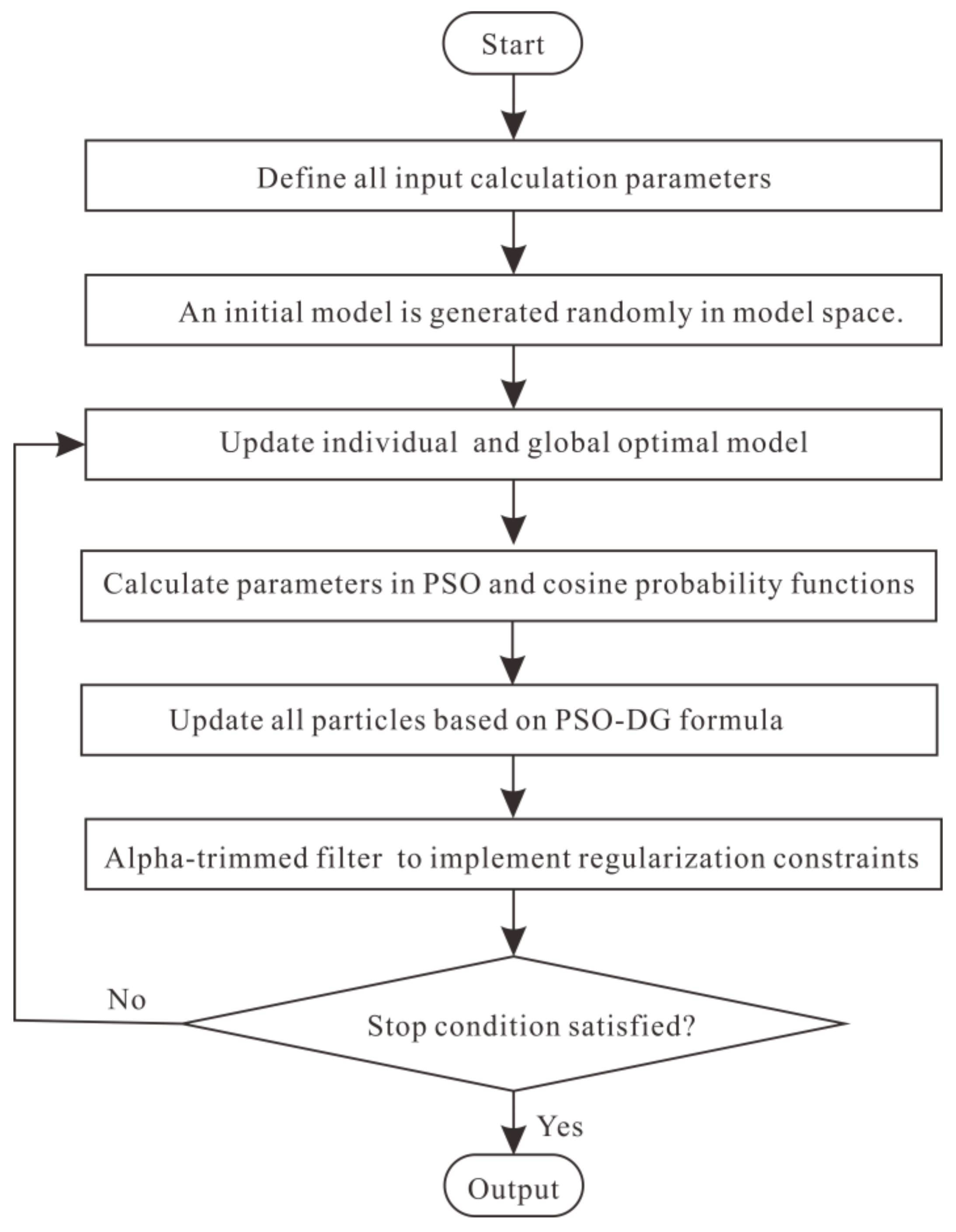
2.2. Theory of the PSO-GD Algorithm

In this section, the original PSO code developed by Miranda (2017) in Python is improved and turned into an HPSO-TVAC [40]. Then, a new model-updating equation is developed based on the correction terms in the PSO and GA models. The PSO and GA algorithms are integrated through a cosine probability function. In addition, the α-trimmed filter is selected as a regularization constraint to smooth the model.

Inspired by the search behavior of bird and fish swarms in nature, Kennedy and Eberhart proposed the PSO algorithm in 1995 [43]. The basic PSO algorithm calculates velocity and location using Equations (10) and (11), respectively.

$$v_i^{t+1}=v_i^t+{\alpha }_1{\gamma }_1\left(P_i-x_i^t\right)+{\alpha }_2{\gamma }_2\left(G-x_i^t\right)$$

(10)

$$x_i^{t+1}=x_i^t+v_i^{t+1}$$

(11)

where ${\gamma }_1$ and ${\gamma }_2$ are random numbers in the range of (0, 1) ${\alpha }_1$ and ${\alpha }_2$ are the individual and social acceleration coefficients, respectively, i is the particle number, k is the current number of iterations, and $P_i$ are the individual optimum solutions, and $G$ is the global optimum solution.

Each particle of the particle swarm may be a possible solution (i.e., an electrical resistivity model) to a short-offset transient electromagnetic (SOTEM) inverse problem. The ability of PSO to escape from local optimum solutions is ascribed to the use of a swarm information sharing system and an individual fitness evaluation system as guidance to correct the model. A continuous search for a better-fitting model for the observation data in the solution space ultimately allows the particles to converge on the optimum solution, which is independent of the selected initial model [45]. When used to solve a 3D inverse problem, the convergence of the PSO algorithm requires many particles and multiple iterations. Therefore, the standard PSO version must be revised. Several variants of the PSO algorithm have been developed to improve the convergence rate [49,50,51,52,53]. The HPSO-TVAC algorithm considerably outperforms the standard PSO algorithm in terms of convergence and stability. The equation of the HPSO-TVAC algorithm is shown as follows:

$$v_i^{k+1}=\omega v_i^k+{\alpha }_1^k{\gamma }_1\left(P_i-x_i^k\right)+{\alpha }_2^k{\gamma }_2\left(G-x_i^k\right)$$

(12)

$$x_i^{k+1}=x_i^k+v_i^{k+1}$$

(13)

In the HPSO-TVAC algorithm, the initial value of α₁ is greater than that of α₂. As the iterative process proceeds, α₁ and α₂ are linearly inverted. The high value of α₁ at the initial stage ensures a global optimization capability, while the high value of α₂ at the final stage ensures the convergence of the swarm towards the optimum solution. α₁ and α₂ are expressed using the following equations:

$${\alpha }_1^k={\alpha }_1^{\max }-\left({\alpha }_1^{\max }-{\alpha }_1^{\min }\right)\left(\frac{k-1}{\max \left(k\right)-1}\right)$$

(14)

$${\alpha }_2^k={\alpha }_2^{\min }+\left({\alpha }_2^{\max }-{\alpha }_2^{\min }\right)\left(\frac{k-1}{\max \left(k\right)-1}\right)$$

(15)

where ${\alpha }^k$ is the acceleration in the current (i.e., kth) iteration, ${\alpha }_1^{\min }$ and ${\alpha }_2^{\min }$ are the minimum values of the individual and social acceleration parameters, respectively, ${\alpha }_1^{\max }$ and ${\alpha }_2^{\max }$ are the maximum values of the individual and social acceleration parameters, respectively, and $\max \left(k\right)$ is the maximum value in the current iteration.

In addition, the following conditions should be considered during the selection of accelerations to ensure stability [40]:

$${\alpha }_1+{\alpha }_2<4$$

(16)

$$\frac{{\alpha }_1+{\alpha }_2}{2}-1<\omega <1$$

(17)

By performing a first-order Taylor series expansion of the linear approximation equation, we obtain the following conventional GD inversion:

$$d_{obs}-e_{obs}\cong G\delta m_{true}+g\left(m_{ref}\right)$$

(18)

where $d_{obs}$ is the observed data, $e_{obs}$ is the observation error, $g$ is considered the response value of parameter $m_{ref}$ in the data-space model, $\delta m_{true}=m_{true}-m_{ref}$, $m_{true}$ is the true geoelectric model, and $m_{ref}$ is an arbitrarily selected electrical resistance model.

Simplification of Equation (18) gives

$$G\delta m_{true}=\delta d_{obs}-e_{obs}$$

(19)

where $\delta d_{obs}=d_{obs}-g(m_{ref})$.

Then, the model correction term is

$$\delta m={\left(G^{T}G\right)}^{-1}{G}^T\delta d$$

(20)

Introducing the model-correction term in the GD algorithm to PSO yields the following equation:

$$v_i^{k+1}=\omega v_i^k+{\alpha }_1^k{\gamma }_1\left(P_i-x_i^k\right)+{\alpha }_2^k{\gamma }_2\left(G-x_i^k\right)+{\alpha }_3^k{\gamma }_3\delta m$$

(21)

$${\alpha }_3^k={\alpha }_3^{\min }+\left({\alpha }_3^{\max }-{\alpha }_3^{\min }\right)\left(\frac{k}{\max \left(k\right)-1}\right)$$

(22)

where ${\alpha }_3^{\min }$ and ${\alpha }_3^{\max }$ are the minimum and maximum values of the gradient descent acceleration parameter, respectively.

To ensure that the global PSO and GD algorithms take precedence at the early and late stages, respectively, a weight-based improvement strategy is further introduced:

$$v_i^{k+1}=\left(1-w^k\right)\left[\omega v_i^k+{\alpha }_1^k{\gamma }_1\left(P_i-x_i^k\right)+{\alpha }_2^k{\gamma }_2\left(G-x_i^k\right)\right]+w^k\left[{\alpha }_3^k{\gamma }_3\delta m\right]$$

(23)

A cosine probability function, $w^k$, which dynamically decays from 1 to 0 as the number of iterations increases, is used as a weighting term to realize a dynamic transition from the GD algorithm to the PSO algorithm. The calculation equation for $w^k$ is given below:

$$w^k=\cos (\frac{\pi }{2}·\frac{k}{\max \left(k\right)})$$

(24)

where $k$ and $\max \left(k\right)$ are the current and maximum numbers of iterations, respectively.

In the PSO-GD algorithm, the GD algorithm guarantees the convergence speed in the early stage, and the global convergence of the PSO algorithm prevents it from falling into a local minimum.

2.2.1. α-Trimmed Filter Constraint

The missing a priori information in an inverse problem and the problem of over stochasticity associated with PSO result in abrupt changes in the information for the model parameters in the inversion result in the 3D space. To address this problem, a regularization constraint term is added to the objective function in a conventional deterministic inversion algorithm, with the goal of stabilizing the inversion process and producing a smooth and reasonable result. The equation of the objective function is as follows:

$$F\left(m\right)=\frac{{\varphi }_0-{\varphi }_c}{{\sigma }_{\varphi }}+\lambda ‖{\log }_{10}\left(\partial m\right)‖$$

(25)

where ${\varphi }_0$ is the observed signal, ${\varphi }_c$ is the calculated response, and λ is referred to as the Lagrangian multiplier or smoothing parameter. The right-hand side of Equation (25) consists of two terms: the first term evaluates the difference between the observed data and the response calculated by the forward simulation model, and the second term realizes the regularization constraint through the minimization of the roughness of the model.

In contrast with conventional model-driven algorithms, a mean filter is generally used to smooth the model during the inversion process of the PSO algorithm equipped with a regularization term [26]. In this study, the α-trimmed filter is used as a regularization constraint strategy for the PSO-GD algorithm. Prior to the start of each iteration, the individual optimum solutions $P_i$ in the particle swarm are successively filtered. First, a fixed window width n is selected based on the scale of the constraint. Then, 3D data centered at the location of the constraint are successively read with a sliding window. The data selected along the x-, y-, and z-axes are sorted in ascending order. Subsequently, a trimming parameter α is selected to trim off the same number of points from the front- and back-end segments of the sequence, with the goal of eliminating the interference from extreme values. Finally, the mean of the remaining points is used as a substitute for the value at the center of the window [54]. The whole process is shown in Figure 1. The 3D filtering equation is as follows:

$$m(n_x,n_y,n_z)=\frac{1}{3\left(n-2\alpha n\right)}\left({\displaystyle \sum _{j=\alpha n+1+n_x}^{n-\alpha n+n_x}\left(m\left(j,n_y,n_z\right)\right)}+{\displaystyle \sum _{j=\alpha n+1+n_y}^{n-\alpha n+n_y}\left(m\left(n_x,j,n_z\right)\right)}+{\displaystyle \sum _{j=\alpha n+1+n_z}^{n-\alpha n+n_z}\left(m\left(n_x,n_y,j\right)\right)}\right)$$

(26)

While smoothing the model, the trim filter can also remove the impact of extreme values, thereby sharpening the boundary information and allowing the anomalies to converge.

To sum up, Figure 2 shows the flowchart of the PSO-GD algorithm developed in this study.

2.2.2. Experimental Function Testing

To evaluate the PSO-GD algorithm, the convergence of a potential function U on the x–y plane is first tested. The equation for U is as follows:

$$U={\displaystyle \sum _{i=1}^n{\left(-2\pi {\sigma }_{1i}{\sigma }_{2i}\sqrt{1-{\rho }_i^2}\right)}^{-1}}\exp \left[\frac{-1}{2\left(1-{\rho }_i^2\right)}\left(\frac{{\left(x-{\mu }_{1i}\right)}^2}{{\sigma }_{1i}^2}+\frac{2\rho \left(x-{\mu }_{1i}\right)\left(y-{\mu }_{2i}\right)}{{\sigma }_{1i}{\sigma }_{2i}}+\frac{{\left(y-{\mu }_{2i}\right)}^2}{{\sigma }_{2i}^2}\right)\right]$$

(27)

Table 1. Parameters of the potential function.

n	${\mathit{\mu }}_1$	${\mathit{\mu }}_2$	${\mathit{\sigma }}_1$	${\mathit{\sigma }}_2$	$\mathit{\rho }$
1	50	25	15	10	0.2
2	60	20	10	20	0
3	75	75	10	12	0.5
4	10	50	60	70	0.1
5	25	66	15	12	−0.2

summarizes the parametric information for U. Figure 3 shows the distribution pattern of the fields, which is characterized by two local minima in the upper half and a global minimum in the lower right corner. The GD, PSO, and PSO-GD algorithms are respectively employed to locate the optimum solution. The optimization capacity of each algorithm is subsequently evaluated based on its optimization result and path. Observation of the optimization results in Figure 3 reveals the following behavior: The PSO and PSO-GD algorithms converge on the global minimum, while the GD algorithm falls into a local minimum. Because the GD algorithm is designed to solve convex optimization problems, its optimization result for a nonconvex optimization problem primarily depends on the selected initial model. The GD algorithm is susceptible to converging on a local minimum near the initial model. In terms of the optimization path, the PSO algorithm searches for an optimum solution in a larger area, which involves a more complex path. When the PSO algorithm eventually converges on the global minimum, its search efficiency considerably decreases as the model approaches the optimum solution. For the PSO-GD algorithm, the addition of the GD information to the model-correction term, to some extent, improves its convergence efficiency near the optimum solution. Therefore, the new algorithm is more effective at executing a global search in the parametric space.

3. Numerical Simulations

The noise immunity and convergence of the PSO-GD algorithm are examined based on two inversion models and are subsequently compared with those of the conventional GD and PSO algorithms.

3.1. Noise Immunity Testing

Figure 4 shows the form of the forward simulation model and transceiver. The height of the sampling point is 50 m. The background electrical resistance in the forward simulation model is 50 Ω·m, while the electrical resistance in the high-resistance anomaly model is 250 Ω·m. The anomaly model has a dimension of 600 m × 600 m × 350 m, with its top surface located at a depth of 250 m. The fundamental frequency and length of the emitter are 12.5 Hz and 2 km, respectively. Samples are collected between 10⁻³ and 20 ms. In addition, Gaussian random noise at 5%, 10%, 20%, and 30% levels is respectively added to the forward simulation data. Analysis of the inversion results in Figure 5 and the fitting error curves in Figure 6 reveals that gradually increasing the noise level increases the number of false anomalies in the inversion result and the fitting error. At a 5% noise level, the inversion result basically matches the true model. At a 10% or 20% noise level, the inversion result can still distinctly show the location and shape of the anomaly. However, this capability is no longer demonstrated at a 30% noise level. Therefore, in practice, reducing the noise level of the input signal as much as possible can help to obtain more information for the geological structure in the inversion result. The overall data noise level should not exceed 20%.

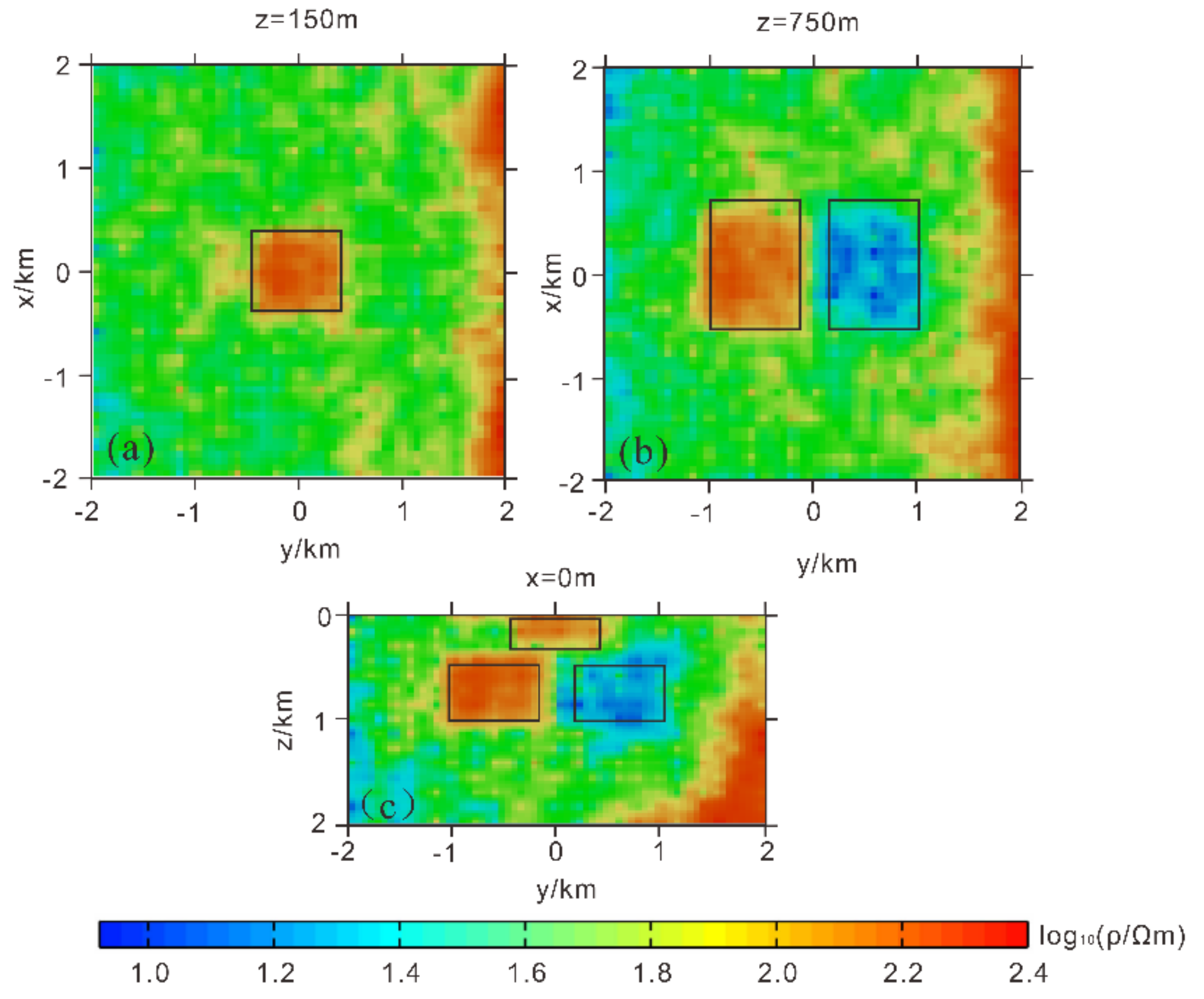
3.2. Complex Model Testing

In this section, the convergence of the PSO-GD algorithm is further examined based on a relatively complex model (see Figure 7), which has a background electrical resistance of 50 Ω·m and contains three anomalies: one shallow high-resistance (250 Ω·m) anomaly, one deep high-resistance (250 Ω·m) anomaly, and one deep low-resistance (10 Ω·m) anomaly. The shallow anomaly has a dimension of 600 m × 600 m × 250 m, with its top surface located at a depth of 20 m. Each of the two deep anomalies has a dimension of 1200 m × 800 m × 500 m, with its top surface located at a depth of 500 m. Gaussian random noise is added at a 20% level to the forward simulation data to generate an inversion-fitting objective. On this basis, the GD, PSO, and PSO-GD algorithms are respectively used to invert the data. A uniform half space with a resistance of 60 Ω·m is used as the initial model for the GD algorithm. Parameter α in the PSO and PSO-GD algorithms is set to 0.2–0.9. The HPSO-TVAC algorithm is used to update the PSO model.

The inversion result yielded by the GD algorithm in Figure 8 can be used to satisfactorily reconstruct the shallow high-resistance structure, but fails to reflect the deep high- and low-resistance anomalies. The inversion result produced by the PSO algorithm in Figure 9 accurately shows the location of each deep anomaly. However, the boundary information for the anomalies requires further correction, and the model is not adequately smooth. In comparison, the inversion result given by the PSO-GD algorithm is smoother and closer to the original model (Figure 10). In addition, note that due to the addition of noise and the relativity of global convergence, some false anomalous points appear in the deep area or at the edges where the constraint on the data decreases in the three inversion results. Figure 11 shows the fitting error curves and uncertainty analysis corresponding to the three algorithms. Compared to the conventional PSO algorithm, the PSO-GD algorithm has a markedly faster convergence rate at the late stage and ultimately yields a smaller fitting error. In an uncertainty analysis, the new algorithm has a higher capacity for model recovery and a more stable effect. This numerical test demonstrates the reliability of the new algorithm in the inversion of SATEM data and lays a foundation for its real-world exploration applications.

4. Case Study

Finally, the 3D PSO-GD inversion technique is employed to process and interpret SATEM measurements of the Qinshui coal mine in Jincheng, Shanxi Province, China. The primary objective of this survey was to investigate the goafs in the No. 3 coal seam of the Permian Shanxi Formation within the survey area to provide a reference for subsequent mining. Water-bearing goafs are a major safety hazard during coal-seam mining. During mining in this survey area of interest, we discovered that water-bearing karst collapse columns pose a threat to the mining project and the safety of the mine.

Based on the available geological and drilling data, as well as the distribution of the formations, a total of 12 SOTEM survey lines, each with a length of 2000 m and an offset from 100–600 m, were designed for the survey area. The emitter had a length of 1700 m and emitted a current with an intensity of 40 A at a fundamental frequency of 12.5 Hz. The flight altitude and speed were set to 50 m and 8 m/s, respectively. The vertical-induced electromotive force dBz/dt was measured. Figure 12 shows the arrangement of the survey lines.

The PSO-GD algorithm was used to perform a 3D inversion. Figure 13 shows the inversion result, which satisfactorily reflects the spatial location of the goafs. The location of the abnormal body is clearly delineated. A vertical profile of the measured line S300 is shown in Figure 14. The known coal seam line is at an approximate height of 400 m, as shown in Figure 14. The results of the inversion made it possible to successfully delimit two abnormal zones of low resistivity and infer the location of the goaf, which will be verified by drilling in the future. Figure 15 shows the data fitting of 1400 points on the measured line S300 and a misfit curve of the 3D data.

5. Conclusions

A new algorithm is presented in this paper based on PSO and GD algorithms and used in 3D inversion of SATEM data. In the new PSO-GD algorithm, PSO ensures stable global convergence at the early stage of inversion, thereby suppressing the multiplicity of solutions associated with inverse problems, while the GD algorithm successfully improves the convergence rate at the late stage of inversion. The new algorithm capably balances the speed and accuracy of the inversion. The PSO and GD algorithms are effectively integrated through a cosine probability function, and the α-trimmed filter used in the PSO-GD algorithm successfully achieves model smoothing. Test results obtained based on simulation and field data show that the new algorithm is a feasible option for 3D inversion and interpretation of SATEM data.

References

1. Smith, R.S.; Annan, A.P.; Mcgowan, P.D. A comparison of data from airborne, semi-airborne, and ground electromagnetic systems. Geophysics 2001, 66, 1379–1385. [Google Scholar] [CrossRef]
2. Mogi, T.; Kusunoki, K.I.; Kaieda, H.; Ito, H.; Jomori, A.; Jomori, N.; Yuuki, Y. Grounded electrical-source airborne transient electromagnetic (GREATEM) survey of Mount Bandai, north-eastern Japan. Explor. Geophys. 2009, 40, 1–7. [Google Scholar] [CrossRef]
3. Ito, H.; Kaieda, H.; Suzuki, K.; Kiho, K.; Mogi, T.; Yuuki, Y.; Jomori, A. A semi-airborne TEM (GREATEM) survey and its applicability to geo-hazards. In Proceedings of the 10th Asian Regional Conference of IAEG (2015), Kyoto, Japan, 26–29 September 2015. [Google Scholar]
4. Ji, Y.; Yang, G.; Guan, S.; Zhang, X.; Tian, P. Interpretation research on electrical source of time domain ground-airborne electromagnetic data. In Proceedings of the World Automation Congress 2012, Puerto Vallarta, Mexico, 4 October 2011. [Google Scholar]
5. Nittinger, C.; Cherevatova, M.; Becken, M.; Martin, T.; Günther, T. A Novel Semi-airborne EM System for Mineral Exploration—First Results from Combined Fluxgate and Induction Coil Data. In Proceedings of the Second European Airborne Electromagnetics Conference, Malmö, Sweden, 3 September 2017. [Google Scholar]
6. Guoqiang, X.; Weiying, C.; Shu, Y. Research study on the short offset time-domain electromagnetic method for deep exploration. J. Appl. Geophys. 2018, 155, 131–137. [Google Scholar] [CrossRef]
7. Wu, X.; Xue, G.; He, Y. The Progress of the Helicopter-Borne Transient Electromagnetic Method and Technology in China. IEEE Access 2020, 8, 32757–32766. [Google Scholar] [CrossRef]
8. Di, Q.Y.; Zhu, R.X.; Xue, G.Q.; Yin, C.C.; Li, X. New development of the Electromagnetic (EM) methods for deep exploration. Chin. J. Geophys. 2019, 62, 2128–2138. [Google Scholar]
9. He, J.S.; Xue, G.Q. Review of the key techniques on short-offset electromagnetic detection. Chin. J. Geophys. 2018, 61, 1–8. [Google Scholar]
10. Wu, X.; Xue, G.Q.; Fang, G.Y.; Li, X.; Ji, Y.J. The Development and Applications of the Semi-Airborne Electromagnetic System in China. IEEE Access 2019, 7, 104956–104966. [Google Scholar] [CrossRef]
11. Li, D.; Tian, Z.; Ma, Y.; Gu, J.; Ji, Y.; Li, S. Application of Grounded Electrical Source Airborne Transient Electromagnetic (GREATEM) System in Goaf Water Detection. J. Environ. Eng. Geophys. 2019, 24, 387–397. [Google Scholar] [CrossRef]
12. Lu, S.; Liang, B.; Wang, J.; Han, F.; Liu, Q.H. 1-D Inversion of GREATEM Data by Supervised Descent Learning. IEEE Geosci. Remote Sens. Lett. 2021, 99, 1–5. [Google Scholar] [CrossRef]
13. Auken, E.; Christiansen, A.V. Layered and laterally constrained 2D inversion of resistivity data. Geophysics 2004, 69, 752–761. [Google Scholar] [CrossRef]
14. Auken, E.; Christiansen, A.V.; Jacobsen, L.; Sørensen, K.I. Laterally Constrained 1D-Inversion of 3D TEM Data. In Symposium on the Application of Geophysics to Engineering and Environmental Problems; Society of Exploration Geophysicists: Tulsa, OK, USA, 2005; pp. 514–518. [Google Scholar]
15. Ley-Cooper, A.Y.; Viezzoli, A.; Guillemoteau, J.; Vignoli, G.; Macnae, J.; Cox, L.; Munday, T. Airborne electromagnetic modelling options and their consequences in target definition. Explor. Geophys. 2014, 46, 74–84. [Google Scholar] [CrossRef]
16. Zhdanov, M.S.; Alfouzan, F.A.; Cox, L.; Alotaibi, A.; Alyousif, M.; Sunwall, D.; Endo, M. Large-scale 3D modeling and inversion of multiphysics airborne geophysical data: A case study from the Arabian Shield, Saudi Arabia. Minerals 2018, 8, 271. [Google Scholar] [CrossRef] [Green Version]
17. McMillan, M.; Haber, E.; Marchant, D. Large scale 3D airborne electromagnetic inversion–recent technical improvements. ASEG Ext. Abstr. 2018, 1, 1–6. [Google Scholar] [CrossRef] [Green Version]
18. Steuer, A.; Smirnova, M.; Becken, M.; Schiffler, M.; Günther, T.; Rochlitz, R.; Yogeshwar, P.; Moerbe, W.; Siemon, B.; Costabel, S.; et al. Comparison of novel semi-airborne electromagnetic data with multi-scale geophysical, petrophysical and geological data from Schleiz, Germany. J. Appl. Geophys. 2020, 182, 104172. [Google Scholar] [CrossRef]
19. Wang, Y. Seismic impedance inversion using I1-norm regularization and gradient descent methods. J. Inverse Ill Posed Probl. 2010, 18, 823–838. [Google Scholar] [CrossRef]
20. Guo, R.; Li, M.; Xiang, C.; Yang, F.; Abubakar, A. 2D Magnetotelluric Inversion using Supervised Descent Method. In Proceedings of the International Applied Computational Electromagnetics Society Symposium—China (ACES), Beijing, China, 29 July–1 August 2018. [Google Scholar]
21. Scales, J.A. Tomographic inversion via the Conjugate Gradient method. Geophysics 1987, 52, 179–185. [Google Scholar] [CrossRef]
22. Hamoda, M.; Mamat, M.; Rivaie, M.; Salleh, Z. A Conjugate Gradient Method with Strong Wolfe-Powell Line Search for Unconstrained Optimization. Appl. Math. Sci. 2016, 10, 721–734. [Google Scholar] [CrossRef]
23. Loke, M.H.; Dahlin, T. A comparison of the Gauss-Newton and quasi-Newton methods in resistivity imaging inversion. J. Appl. Geophys. 2002, 49, 149–162. [Google Scholar] [CrossRef] [Green Version]
24. Dai, M.X.; Chen, J.B.; Cao, J. 1-Regularized full-waveform inversion with prior model information based on orthant-wise limited memory quasi-Newton method. J. Appl. Geophys. 2017, 142, 49–57. [Google Scholar] [CrossRef]
25. Parsopoulos, K.E.; Vrahatis, M.N. Applications in Bioinformatics and Medical Informatics. In Particle Swarm Optimization and Intelligence (Advances and Applications); IGI global: Hershey, PA, USA, 2010; Volume 9, pp. 204–221. [Google Scholar] [CrossRef]
26. Sen, M.K.; Stoffa, P.L. Global Optimization Methods in Geophysical Inversion; Cambridge University Press: Cambridge, UK, 2013. [Google Scholar] [CrossRef]
27. Rosas-Carbajal, M.; Linde, N.; Kalscheuer, T.; Vrugt, J.A. Two-dimensional probabilistic inversion of plane-wave electromagnetic data: Methodology, model constraints and joint inversion with electrical resistivity data. Geophys. J. Int. 2014, 196, 1508–1524. [Google Scholar] [CrossRef] [Green Version]
28. Hauser, J.; Gunning, J.; Annetts, D. Probabilistic inversion of airborne electromagnetic data under spatial constraints. Geophysics 2015, 80, E135–E146. [Google Scholar] [CrossRef]
29. Hansen, T.M.; Minsley, B.J. Inversion of airborne EM data with an explicit choice of prior model. Geophys. J. Int. 2019, 218, 1348–1366. [Google Scholar] [CrossRef]
30. Bai, P.; Vignoli, G.; Viezzoli, A.; Nevalainen, J.; Vacca, G. (Quasi-) Real-Time Inversion of Airborne Time-Domain Electromagnetic Data via Artificial Neural Network. Remote Sens. 2020, 12, 3440. [Google Scholar] [CrossRef]
31. Feng, B.; Zhang, J.F.; Li, D.; Bai, Y. Resistivity-depth imaging with the airborne transient electromagnetic method based on an artificial neural network. J. Environ. Eng. Geophys. 2020, 25, 355–368. [Google Scholar] [CrossRef]
32. Noh, K.; Yoon, D.; Byun, J. Imaging subsurface resistivity structure from airborne electromagnetic induction data using deep neural network. Explor. Geophys. 2020, 51, 214–220. [Google Scholar] [CrossRef]
33. Puzyrev, V.; Swidinsky, A. Inversion of 1D frequency-and time-domain electromagnetic data with convolutional neural networks. Comput. Geosci. 2021, 149, 104681. [Google Scholar] [CrossRef]
34. Minsley, B.J.; Foks, N.L.; Bedrosian, P.A. Quantifying model structural uncertainty using airborne electromagnetic data. Geophys. J. Int. 2021, 224, 590–607. [Google Scholar] [CrossRef]
35. Cheng, J.L.; Li, M.X.; Xiao, Y.L.; Sun, X.Y.; Chen, D. Study on particle swarm optimization inversion of mine transient electromagnetic method in whole-space. Chin. J. Geophys. 2014, 57, 3478–3484. [Google Scholar]
36. Li, H.; Xue, G.; He, Y. Decoupling induced polarization effect from time domain electromagnetic data in Bayesian framework. Geophysics 2019, 84, A59–A63. [Google Scholar] [CrossRef]
37. Yang, L.; Sun, B.; Sun, X. Inversion of Thermal Conductivity in Two-Dimensional Unsteady-State Heat Transfer System Based on Finite Difference Method and Artificial Bee Colony. Appl. Sci. 2019, 9, 4824. [Google Scholar] [CrossRef] [Green Version]
38. Song, T.; Hu, X.; Du, W.; Cheng, L.; Xiao, T.; Li, Q. Lp-Norm Inversion of Gravity Data Using Adaptive Differential Evolution. Appl. Sci. 2021, 11, 6485. [Google Scholar] [CrossRef]
39. Pace, F.; Santilano, A.; Godio, A. A Review of Geophysical Modeling Based on Particle Swarm Optimization. Surv. Geophys. 2021, 42, 505–549. [Google Scholar] [CrossRef] [PubMed]
40. Pace, F.; Santilano, A.; Godio, A. Particle swarm optimization of 2D magnetotelluric data. Geophysics 2019, 84, E125–E141. [Google Scholar] [CrossRef]
41. Fernández-Álvarez, J.P.; Fernández-Martínez, J.L.; García-Gonzalo, E.; Menéndez-Pérez, C.O. Application of the particle swarm optimization algorithm to the solution and appraisal of the Vertical Electrical Sounding inverse problem. In Proceedings of the 11th Annual Conference of the International Association of Mathematical Geology (IAMG’06), Liège, Belgium, 12–14 June 2006. [Google Scholar]
42. Shaw, R.; Srivastava, S. Particle swarm optimization: A new tool to invert geophysical data. Geophysics 2007, 72, 781–786. [Google Scholar] [CrossRef]
43. Martínez, J.; Gonzalo, E.; Álvarez, J.; Kuzma, H. PSO: A powerful algorithm to solve geophysical inverse problems: Application to a 1D-DC resistivity case. J. Appl. Geophys 2010, 71, 13–25. [Google Scholar] [CrossRef]
44. Cheng, J.; Li, F.; Peng, S.; Sun, X.; Zheng, J.; Jia, J. Joint inversion of TEM and DC in roadway advanced detection based on particle swarm optimization. J. Appl. Geophys. 2015, 123, 30–35. [Google Scholar] [CrossRef]
45. Olalekan, F.; Di, Q. Particle Swarm Optimization Method for Stochastic Inversion of MTEM Data. IEEE Geosci. Remote Sens. Lett. 2018, 15, 1832–1836. [Google Scholar] [CrossRef]
46. Liu, S.; Liang, M.; Hu, X. Particle swarm optimization inversion of magnetic data: Field examples from iron ore deposits in ChinaParticle swarm optimization inversion. Geophysics 2018, 83, J43–J59. [Google Scholar] [CrossRef]
47. Hyman, J.M.; Shashkov, M. Mimetic Discretizations for Maxwell’s Equations. J. Comput. Phys. 1999, 151, 881–909. [Google Scholar] [CrossRef] [Green Version]
48. Cockett, R.; Kang, S.; Heagy, L.J.; Pidlisecky, A.; Oldenburg, D.W. SimPEG: An open source framework for simulation and gradient based parameter estimation in geophysical applications. Comput. Geosci. 2015, 85, 142–154. [Google Scholar] [CrossRef] [Green Version]
49. Miranda, L.J. PySwarms: A research toolkit for Particle Swarm Optimization in Python. J. Open Source Softw. 2018, 3, 433. [Google Scholar] [CrossRef] [Green Version]
50. Kennedy, J.; Eberhart, R. Particle swarm optimization. In Proceedings of the International Conference on Neural Networks IV, Perth, WA, Australia, 27 November–1 December 1995. [Google Scholar]
51. Ratnaweera, A.; Halgamuge, S.K.; Watson, H.C. Self-Organizing Hierarchical Particle Swarm Optimizer with Time-Varying Acceleration Coefficients. IEEE Trans. Evol. Comput. 2004, 8, 240–255. [Google Scholar] [CrossRef]
52. Zhan, Z.H.; Zhang, J. Adaptive Particle Swarm Optimization. In Proceedings of the International Conference on Ant Colony Optimization and Swarm Intelligence, Brussels, Belgium, 22–24 September 2008. [Google Scholar]
53. Pallero, J.L.G.; Fernández-Martínez, J.L.; Bonvalot, S.; Fudym, O. 3D gravity inversion and uncertainty assessment of basement relief via Particle Swarm Optimization. J. Appl. Geophys. 2017, 139, 338–350. [Google Scholar] [CrossRef]
54. Bednar, J.; Watt, T. Alpha-trimmed means and their relationship to median filters. IEEE Trans. Acoust. Speech Signal Processing 1984, 32, 145–153. [Google Scholar] [CrossRef]
Figure 1. Schematic diagram of the α-trimmed constraint (n = 5, α = 0.25).
Applsci 12 03042 g001
Figure 2. Flowchart of the PSO-GD algorithm.
Applsci 12 03042 g002
Figure 3. Optimization paths of the (a) GD, (b) PSO, and (c) PSO-GD algorithms.
Applsci 12 03042 g003
Figure 4. Schematic diagrams of the transceiver and the position of the anomaly.
Applsci 12 03042 g004
Figure 5. Horizontal sectional views of the inversion results at different noise levels (z = 500 m).
Applsci 12 03042 g005
Figure 6. Convergence of the residual errors of the fits at different noise levels.
Applsci 12 03042 g006
Figure 7. Schematic diagrams of the transceiver and the locations of the anomalies.
Applsci 12 03042 g007
Figure 8. Inversion result yielded by the GD algorithm. (a) Horizontal sectional view at z = 150 m. (b) Horizontal sectional view at z = 750 m. (c) Vertical sectional view at x = 0 m.
Applsci 12 03042 g008
Figure 9. Inversion result yielded by the PSO algorithm. (a) Horizontal sectional view at z = 150 m. (b) Horizontal sectional view at z = 750 m. (c) Vertical sectional view at x = 0 m.
Applsci 12 03042 g009
Figure 10. Inversion result yielded by the PSO-GD algorithm. (a) Horizontal sectional view at z = 150 m. (b) Horizontal sectional view at z = 750 m. (c) Vertical sectional view at x = 0 m.
Applsci 12 03042 g010
Figure 11. Fitting error curves and uncertainty analysis. (a) Fitting error curves. (b) uncertainty analysis.
Applsci 12 03042 g011
Figure 12. Map of the survey area.
Applsci 12 03042 g012
Figure 13. 3D inversion result produced by the PSO-GD algorithm.
Applsci 12 03042 g013
Figure 14. Vertical sectional view of the 3D inversion of the measurement taken on the S300 survey line.
Applsci 12 03042 g014
Figure 15. Field data fitting. (a) Data fitting. (b) Fitting error curve.
Applsci 12 03042 g015