Article

A Data Processing Framework for Polar Performance Diagrams

by
Valentin Dannenberg
*,†,
Robert Schüler
*,† and
Achill Schürmann
*,†
Institute of Mathematics, University of Rostock, 18051 Rostock, Germany
*
Authors to whom correspondence should be addressed.
These authors contributed equally to this work.
Appl. Sci. 2022, 12(6), 3085; https://doi.org/10.3390/app12063085
Submission received: 9 December 2021 / Revised: 3 March 2022 / Accepted: 14 March 2022 / Published: 17 March 2022
(This article belongs to the Special Issue Robotic Sailing and Support Technologies)

Abstract

:
Polar performance diagrams are commonly used to predict the performance of a sailing vessel under given wind conditions. They are, in particular, an essential part of robotic sailing vessels and a basis for weather routing algorithms. In this paper we introduce a new framework for scientific work with such diagrams, which we make available as an open source Python package. It contains a model for the creation of polar performance diagrams from measurement data and supports different representations of polar performance diagrams for different tasks. The framework also includes several methods for the visualisation of polar performance diagrams, for example for scientific publications. Additionally, the presented framework solves basic tasks for the future development of weather-routing algorithms in a far more general manner than other methods did previously: it provides the calculation of costs of a sailing trip using custom cost functions, suggestions of optimal steering using convex hull calculations and a more flexible calculation of isochrone points, using custom weather models. Altogether, the presented framework allows future researchers to more easily handle polar performance diagrams. The corresponding Python package is compatible with various established file formats.

1. Introduction

A natural occurring task when steering a sailing vessel is to predict the speed over ground (SOG) in a given direction and in a given situation. This prediction is a difficult physical problem ([1,2]) and depends on various factors, including wind, current, waves and the shape of the vessel, but also the competence of the crew, among others.
For simplification, one can assume idealised conditions for some of these factors (e.g., that there is no current and no waves) and finitely many possibilities for others (e.g., the used set of sails or the shape of the hull). In this way, the complicated physical dependencies can be simplified to finitely many different functions depending only on a few parameters. Traditionally, this method is used to describe the performance of a boat in dependency of strength and direction of the wind, yielding a polar (performance) diagram.
These polar diagrams are also a fundamental part of computer-assisted and robotic sailing (see for instance [3,4]) and a basic tool used in routing software for sailing vessels [5,6].
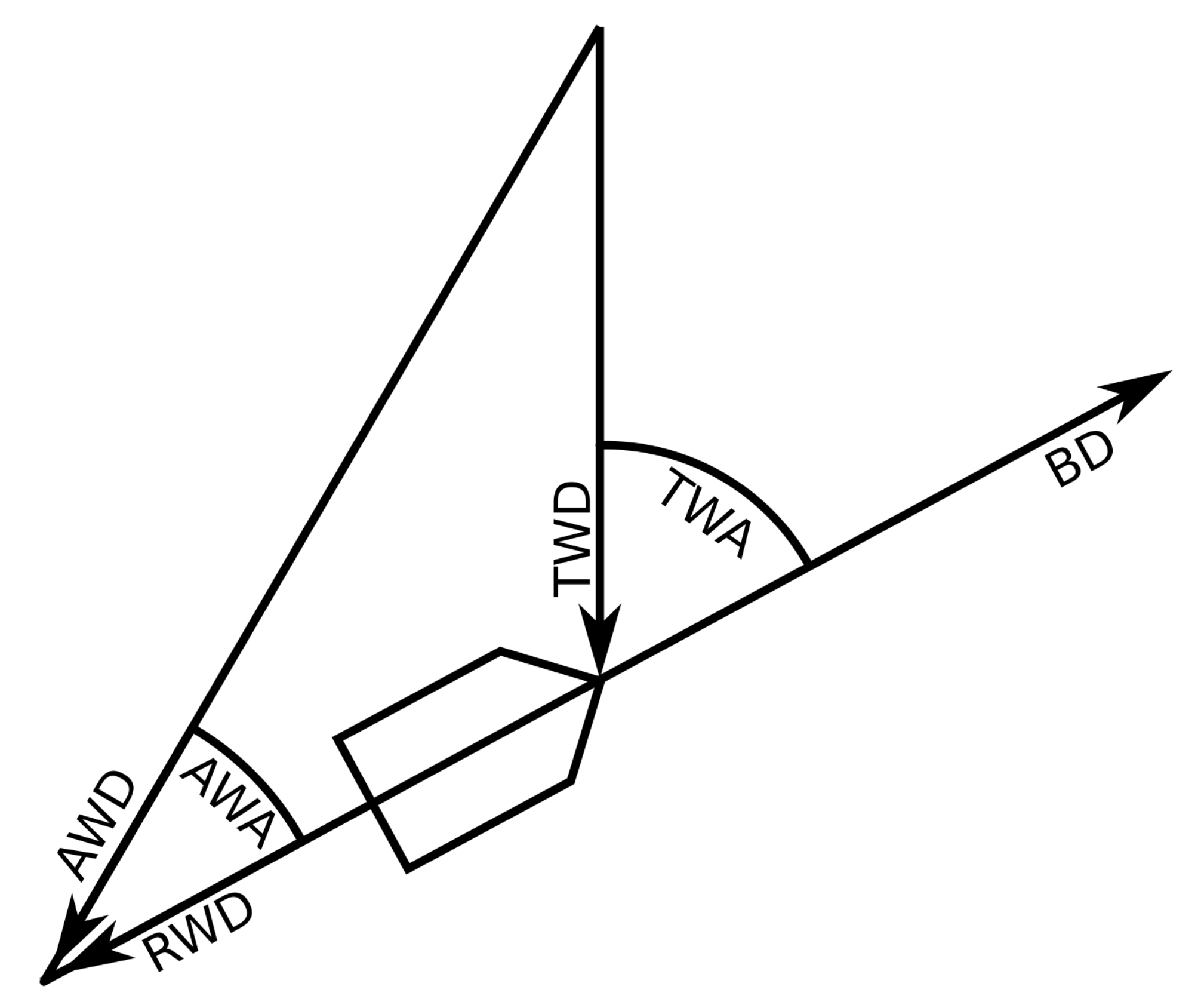
They predict the performance (boat speed/speed through water/BSP) of a sailing vessel under fixed circumstances (usually using a fixed set of sails) and under idealised conditions (usually no current and wave effects are captured, in this case BSP ≈ SOG). In their most common form, they predict BSP for a given true wind angle and true wind speed (TWA/TWS). Often, a polar diagram is visualised as a table or as a polar plot of BSP in dependency of TWA, with different curves indicating specific values of TWS (see Figure 1 or Figure 5 in  [7]). Sometimes, apparent wind is used instead of true wind (for example in [8]), but for the purpose of this paper, a polar diagram always uses true wind. For a better understanding of the different terms, see Figure 2 or [1,2].
Polar diagrams given by manufacturers or by official sailing organisations such as the Offshore Sailing Congress (ORC) are mostly obtained by Velocity Prediction Programs (VPPs) that use computer simulations to predict the boat performance under idealised theoretical conditions [9]. For an overview of naval architecture, VPPs and alternatives refer to [10,11] or [12]. However, it is not always reasonable to use a VPP, since real conditions can differ a lot from the assumed idealized conditions (e.g., the condition of the boat, the sails etc.). Thus, the real performance of the vessel might differ notably from the prediction. An obvious alternative approach is to measure wind and performance under real conditions and estimate a polar diagram from this information [13]. Polar diagrams obtained in this way can provide a more realistic picture of the performance under usual conditions. However, additional statistical and practical obstacles have to be considered.
In this paper we introduce a new framework, which simplifies the scientific work with polar diagrams. We also present a corresponding Python package, hrosailing. The novelty of the framework is that it supports a scientific approach to polar diagrams. In contrast to established user-focused tools, the hrosailing framework provides a lot more transparency and customisability. In particular the framework contains:
  • different representations of polar diagrams for different purposes;
  • a pipeline model for the modular creation of polar diagrams from real-world data;
  • different methods of visualisation, for example for scientific publications;
  • suggestions for optimal steering using convex hull computations;
  • computation of travelling cost (with custom cost functions) considering the weather conditions at each point;
  • computation of isochrone points, considering the weather conditions at each point;
  • a modular design for easy extensions and customisations;
  • lastly, our Python package is compatible with several established data formats and Python libraries.
Our paper is organised as follows: In Section 2 we formulate the problems and give some theoretical background. Then, we introduce the hrosailing framework in Section 3 and discuss how the problems of the previous section are addressed. In Section 4 we give a description of the corresponding Python implementation, namely the hrosailing package, followed by a brief description of a real case study in Section 5. We end this paper in Section 6 with conclusions and with a brief discussion of possible future work.

2. Problem Formulations and Theoretical Backgrounds

In its purest mathematical form, polar diagrams are (partial) functions mapping ( TWA , TWS ) pairs to BSP values. We sometimes use the notation BSP ( TWA , TWS ) to refer to this function. Since functions with two-dimensional input are harder to handle, the TWS value often will be fixed, reducing the polar diagram to a function of TWA to BSP. Such a reduced function is called a slice of the polar diagram at a certain constant TWS. A slice is traditionally visualised by a polar plot.
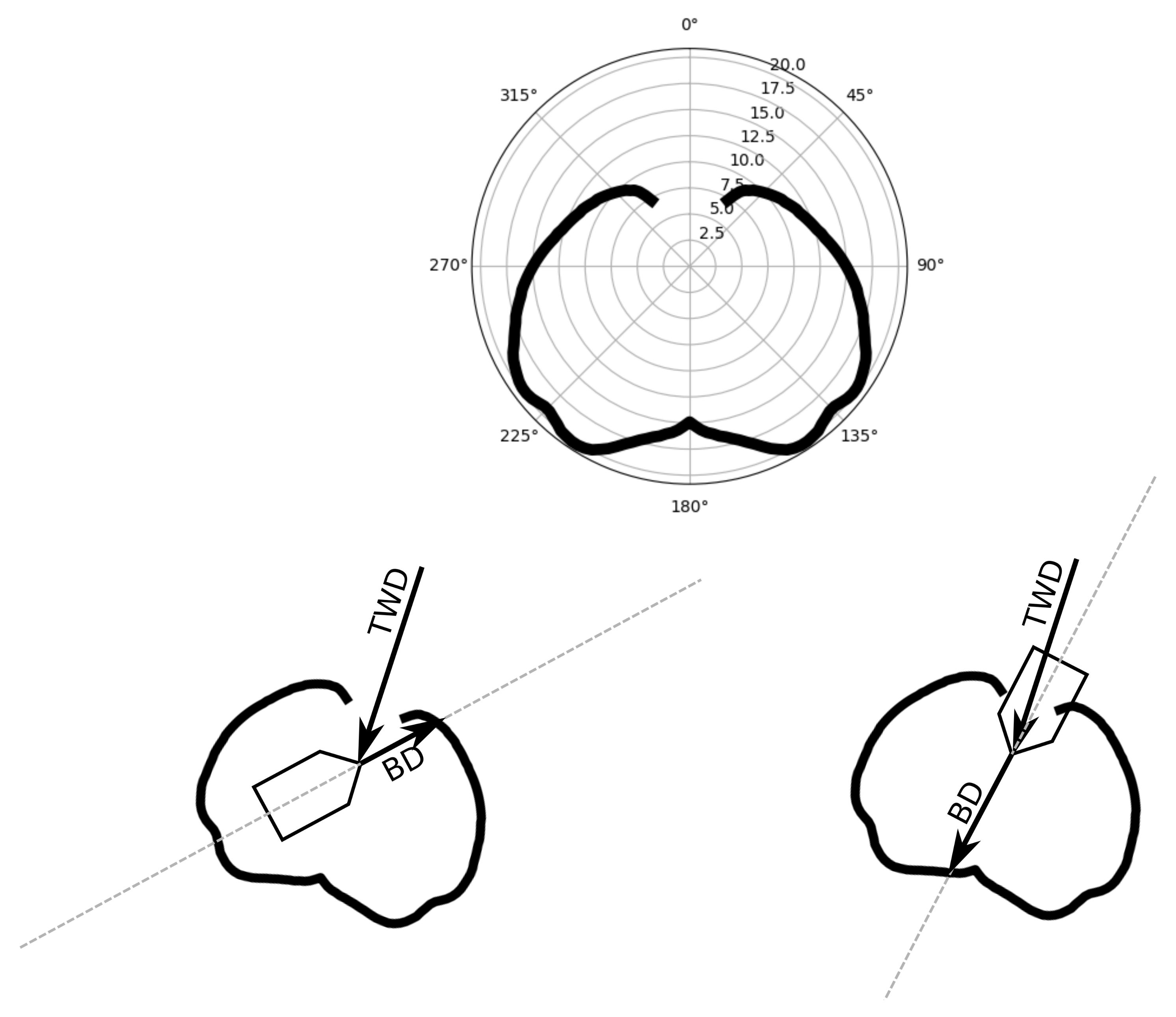
In addition to the natural interpretation, we can also use the following interpretation of a polar diagram slice: we imagine the TWS and the wind direction to be fixed (from top to bottom in the polar diagram); then, the polar plot gives us the exact boat direction vectors (BD) for each possible direction the vessel could take (see Figure 3).

2.1. Representations for Different Purposes

In reality, it is impossible to find the real polar diagram as a function since there can only be a finite amount of measurements. It is still possible to use methods from data science (see also Section 2.3) for an approximation. Nevertheless, specific representations might be favourable in specific situations. In many applications and even on sailing vessels themselves, it is common to use a table to describe a polar diagram, with rows corresponding to specific values of TWA, columns corresponding to specific values of TWS and entries corresponding to BSP. For compatibility reasons, it may be preferable to have your polar diagram in such a format. On the other hand, a data scientist might end up with other types of data when using different data science tools, such as interpolation or regression.
Therefore, it is natural to use different representations of polar diagrams to serve different requirements. To the best of our knowledge, common tools only support the table option.

2.2. Evaluation and Visualisation

Given any representation of a polar diagram, we should be able to evaluate the predicted BSP for a given TWA and TWS.
Furthermore, the human brain processes abstract information better when it is visualised properly. We aim to include a multitude of different visualisations in the presented framework, including new ones that are not commonly used so far.

2.3. From Real World Data to Polar Diagrams

As mentioned before, one way to obtain polar diagrams which reflect the real-world conditions of a given sailing vessel is to make extensive measurements and use techniques from data science to construct a polar diagram from them. When measuring real-world sailing data, there are effects from factors that have been assumed to be idealised (such as currents and waves) and measurement errors. Furthermore, the polar diagram should only contain information of the maximum boat speeds, where in reality there are phases of acceleration and the top speed is only obtained after a certain amount of time. Thus, the data obtained from real-world measurements inevitably contains errors and inaccuracies and needs to be handled carefully.
Furthermore, different types of sailing vessels produce different kinds of polar diagrams. Therefore, a relevant problem is to find a flexible, customisable data-processing model, specialised for the creation of polar diagrams. To the best of our knowledge, such a data-processing model has not yet been discussed in the literature.

2.4. Optimal Manoeuvres

It is well known to every sailor that tacks and jibes can be used to reach your destination faster than by sailing to your destination on a straight course. This is especially true when sailing “with” or “against” the wind.
This naturally yields the following problem: For fixed wind conditions, which manoeuvres should we plan in order to minimise the time needed?
Often a ship has different sets of sails with different properties to use. Then the question is extended to: which manoeuvres and sail changes should we plan in order to minimise the time needed?

2.5. Weather Routing—An Application of Polar Diagrams

The task of weather routing comes naturally when steering a sailing vessel for a longer period of time. We assume that wind (and other factors such as geographical information, current, waves, etc.) are dependent on time and position, and the velocity of our vessel can be predicted at any given time and position. Of course, in reality a weather forecast relies on statistics and interpolation and is never 100% reliable. A simple question is: what is the best course to take from one position to another? The term “best course”, in its simplest form, refers to the fastest path. However, more convoluted cost functions, considering more factors (such as safety), can also be used (see [6,14]).
We continue to discuss two standard approaches to solve a weather-routing problem and some related problems. For a more detailed overview we refer to [15,16].

2.5.1. Graph Based Algorithms

The main idea of graph-based algorithms is to use a predefined set of positions (often a grid representation of a flat map) as graph nodes and a set of rules declaring between which nodes the vessel can travel to generate the edges(see Figure 4 or Figure 2 in  [14] for an example).
After assigning weights to the edges which correspond to a cost function, this results in a weighted graph. On this graph, standard shortest path algorithms, such as Dijkstra or A* can be applied to find an optimal path.
The question how to assign weights to the edges occurs naturally. Most of the established tools assume one can travel from A to B with constant weather conditions given at the start of the tour and calculate the costs under this assumption. We aim to include the calculations of edge weights for general cost functions in our framework considering the weather conditions at each point.

2.5.2. Isochrone Methods

The main idea of approaches subsumed under the label isochrone methods is to iteratively find samples of positions which can be reached in a predefined amount of time from already-explored positions (see [17]). To reduce complexity, positions which do not seem profitable are dismissed on the way. If the final destination is covered by the isochrones, an optimal path can be traced back. An illustration of the isochrone approach is given by Figure 5 (see also [18]).
An important task when running such an algorithm is to find positions which can be reached in a predefined time in a given direction. To be precise, for a given starting position A, a direction w and a predefined total time c, we aim to find the distance s we need to travel from A in direction w, such that t ( s ) = c . Here, t ( s ) is defined as before. The established way is to calculate isochrone points by assuming the weather conditions given at the starting point. We aim to include an algorithm in our framework which can compute isochrone points while considering the changing weather conditions along the way.

3. The hrosailing Framework

In this section we discuss the hrosailing framework and how it solves the problems introduced in Section 2. Detailed discussions of different aspects of the framework are explained in the following subsections. For a visual overview of the framework, we refer to Figure 6.

3.1. Representation for Different Purposes

The established approach to represent polar diagrams is via a table of boat speeds where the rows and columns are indexed by certain wind speeds and wind angles. These kinds of polar diagrams are compatible with a range of other tools and software, but are hard to adjust to real-world data. For example, if we obtained very good measurement data for some wind speeds and angles and very poor data for others, this information would possibly be lost in a table.
Another possibility is just to save triplets of ( TWA , TWS , BSP ) data points that are supposed to be of good quality (for example generated by filtering and interpolating). This representation reflects the quality of the underlying data very well.
As a result of a regression analysis, or to ensure certain theoretical behaviours of your polar diagram, it may be favourable to represent your polar diagram as a function BSP ( TWA , TWS ) of a given type (approximating the real underlying function).
The three kinds of representations discussed above are included in the hrosailing framework as PolarDiagramTable, PolarDiagramPointCloud and PolarDiagramCurve, respectively.
Each of these formats has some advantages and disadvantages. We can compare these by the following criteria:
  • Can a human (trained in sailing), with a printed version of the raw data, easily use the polar diagram to suggest optimal steering of the corresponding vessel?
  • Can a human (not trained in programming) at least read and understand a printed version of the data?
  • Can the data be used in conjunction with other software such as OpenCPN [19]?
  • Is the computation of a BSP value for given (TWA, TWS) values independent of interpolation methods?
  • Can the polar diagram easily be adapted when new information is given?
  • Are the respective polar plots smooth and therefore (possibly) more realistic?
  • Is there nearly complete information for a collection of slices?
  • Theoretically, is the polar diagram capable to adapt to (probably incomplete) real world measurement data?
A complete comparison with respect to these criteria is given in Table 1. By changing the sails, the polar diagram of a vessel also changes drastically. Many vessels can switch between different sets of sails for different weather conditions. In order to understand the overall behaviour of a vessel, a collection of polar diagrams for each sets of sails is desirable. This is also included in the hrosailing framework as PolarDiagramMultisails.

3.2. Evaluation and Visualisation

As mentioned in Section 2.2, the hrosailing framework contains multiple methods of evaluation and visualisation. The evaluation of polar diagrams is simple if we have a PolarDiagramCurve, since it is equivalent to the evaluation of the respective function. In the cases of PolarDiagramTable or PolarDiagramPointCloud, there are many pairs (TWA, TWS) without a corresponding BSP value. In these cases, we evaluate the polar diagram PD with the use of an interpolation method I, say
BSP ( TWS , TWA ) I ( PD , TWS , TWA ) .
There are several well-established interpolation methods [20], but since this framework is designed for academic purposes, we prefer not to choose a specific one.
The established visualisation of polar diagrams is as polar plots of one or more slices. In some cases, other forms of visualisation might be preferable. If a data scientist is trying to choose a good model function in order to perform a regression analysis, a regular plot of one or more slices would be more helpful. In Section 3.4 we will discuss that the convex hull of slices has an important role for optimal steering. For a better understanding of the optimal steering, a plot of one or more convex hulls of slices is preferable. To obtain a good understanding of the polar diagram as a function in two arguments, a three-dimensional plot is useful (at least on a computer where we can rotate the plot). For a more pleasing visualisation of the complete polar diagram that can be printed, we suggest the use of a colour gradient plot, with axes TWS and TWA and the colour corresponding to BSP.
The hrosailing framework contains these five types of visualisations. With these tools, researchers are in a good position to analyse and present their polar diagrams. Note that in this paper, most visualisations have been obtained using the hrosailing package.

3.3. From Real World Measurements to Polar Diagrams

As a part of the hrosailing framework we introduce our pipeline model, a modular model designed for easy and flexible data processing. Data processing often involves similar steps, and not every researcher should be required to start this process from zero. Especially in the case of polar diagram generation, there are some additional heuristics which can be used. The main idea is to carefully choose defaults that will produce, in most cases, acceptable results. In order to improve the results, a researcher can only modularly modify some steps (such as exchanging the pipes of a pipeline) while the other steps remain at their default functionality.
In the following, we explain our pipeline model in some detail (see also Figure 7). Real-world sailing data can come in different forms, for example as NMEA sentences (see [21]), other file formats or arrays. Thus, the data needs to be transformed into a standard format (by a DataHandler) for further processing. The format used by the hrosailing framework is a measurement table where each row corresponds to a point in time and each column corresponds to a measured quality.
In some cases, we have a good (or sufficient) understanding of how to calculate some values from the data. As an example: assume you have recorded some data including the current and want to eliminate the respective effect by a simple vector subtraction on the boat direction. Such computations (done by an InfluenceModel) are the next step of the data-handling pipeline.
The following two steps together deal with data that, due to real world effects, probably contain errors. First of all, a method (Weigher) is used to evaluate the quality of every measurement and assigns a corresponding weight to it. The Weigher thereby produces data points with only 4 entries, namely TWS, TWA, BSP and the weight of the data point. The generated weights can then be used for the rest of the processing.
In the next step (Filter), data which probably does not contain useful information is deleted (preferably according to the weights assigned before). After this step, you also can create artificial data points modelling the expected behaviour of a polar diagram obtained, for example, from theory. By default, additional data points with weight 1 which indicate that you can not sail directly against the wind are added.
After these first steps, the pipeline has produced three-dimensional data points that are preprocessed, weighted and filtered. To obtain a polar diagram from this, the process needs to be extended further, depending on the representation of polar diagram you wish to obtain. In order to do this, the hrosailing framework provides the notion of a PipelineExtension which takes weighted points and produces a polar diagram (see also rows 2–4 in Figure 7). While the framework predefines an extension for every supported kind of representation, a researcher may append their own extension to the pipeline. The hrosailing framework contains three predefined extensions, one for each supported polar diagram representation. A TableExtension produces a PolarDiagramTable from given wind speed and wind angle resolution by applying an interpolation method on a neighbourhood of the data points. In other words, for resolutions [ TWS 1 , , TWS n ] , [ TWA 1 , , TWA m ] the corresponding boat speeds are calculated with an interpolation method I and a neighbourhood N : R 2 2 R 2  as
BSP i , j = I ( TWS i , TWA j , S i , j )
where
S i , j = { ( TWS , TWA , weight ) WPTS : ( TWS , TWA ) N ( TWS i , TWA j ) } .
The PointCloudExtension basically works in the same way, except that the (TWS, TWA) pairs, which have to be interpolated, are generated first by a sampling method. You can also apply the CurveExtension which generates a PolarDiagramCurve from weighted points via regression.
While the framework can always be extended by customised methods, the following basic tools are included:
  • DataHandler for csv-files, arrays and files containing NMEA sentences;
  • CylindricMeanWeigher which produces higher weights for points whose BSP is roughly the mean of the BSP points in a given cylindric neighbourhood and
    CylindricMemberWeigher which produces higher weights for points with more neighbours in a cylindric neighbourhood;
  • FluctuationWeigher which assigns low weights for data which strongly fluctuates in time (locally) and high weights for data which is nearly constant in time (also locally);
  • BoundFilter which only keeps points whoose weights surpass a given threshold and QuantileFilter which keeps a given percentage of the weighed points;
  • classical interpolators, such as the inverse distance interpolator for nongridded data and the improved inverse distance interpolator [20];
  • a more general interpolator, namely the ArithmeticMeanInterpolator, i.e., I calculates the weighted mean with weights e α w | ( TWS , TWA ) ( s , a ) | for each point ( s , a , w ) WPTS ;
  • least square regression methods (Section 2.2.1 of  [22]) and orthogonal distance methods [23];
  • sampling methods such as Fibonacci samples (inspired by [24]) and Archimedean samples (inspired by [25]), these produce sample points in the convex hull of available (TWS, TWA) data points with equidistantly distributed angles on the spiral
    β ( cos ( β ) , sin ( β ) ) and equidistantly distributed points on the spiral β ( cos ( β ) , sin ( β ) ) respectively;
  • neighbourhoods such as Ball, Ellipsoid, Cuboid or Polytope;
  • multiple model functions representing common types of polar diagrams.
To conclude, the introduced pipeline model contains a range of flexible tools for handling different types of issues that might occur when processing the sailing data. To the best of our knowledge, established tools only provide ways to generate polar diagrams by a “black box” function.

3.4. How to Use the Convex Hull of a Polar Diagram Slice for Optimal Manoeuvres

The use of the convex hull for optimal manoeuvres is a well-known fact in the sailing community, but has never been formulated as part of a data-handling framework.
In its simplest form, a polar diagram gives us information about the possible boat speed for given values of TWA and TWS under some further assumptions, without planning tacks or jibes. If we allow tacks and jibes (or changing of sails), the sailing vessel can outperform these speeds in some directions.
For given TWS, a diagram representing the top performance in a direction allowing manoeuvres can be constructed as follows: first, take the convex hull of the polar plot of the respective slice, that is the smallest convex set containing the polar plot; then, for each direction, choose the point in the convex hull which is farthest away from the origin. The resulting diagram is the one giving the top performance aimed for. It can be read in a similar way to the usual polar plot of a slice (see Figure 8).
It is also possible to get an exact description of the manoeuvre necessary to obtain the respective top performance. To do this, first note that in our situation any point p on the boundary of the convex hull is either a point of the initial set or can be expressed as p = λ v + ( 1 λ ) w = w + λ ( v w ) , where v and w are points of the boundary of the initial set and 0 λ 1 . In other words, the point p is on a segment between two boundary points v and w of the initial set and λ = | p w | | v w | determines the exact position on the segment. If p is on the boundary of the initial polar diagram, it is sufficient to simply steer in the respective direction. Otherwise, an optimal course would be to steer at a ratio of λ of the time in the direction of v and a ratio of ( 1 λ ) of the time in the direction of w.
Often a ship has different sails which can be used. In these cases, we need a polar diagram for each possible setting of sails. Then, we can use the same argumentation as above applied to the convex hull of the union of the respective polar plots of slices. The corresponding strategy then may involve a change of sails (see Figure 9).
For this construction to be precise, we have to make some idealised assumptions. First of all, we assume that the polar diagram precisely describes the capabilities of the boat. Since we are using the best available polar diagram, this assumption is reasonable. Secondly, we assume that the wind conditions are constant in time and position. This assumption is only reasonable if the weather is suitably stable. Lastly, we assume that a direction change can be done without loss of velocity. This assumption can be motivated in particular for longer periods of travel (and with as few direction changes as possible), since then these effects become neglectable.
To summarise, these kinds of calculations work well if the wind conditions are relatively stable and we keep directions for a reasonable amount of time. In other situations, it may be favourable to use weather routing instead.

3.5. Weather Model

In many applications, such as weather routing, it is necessary to use predictions of the weather conditions. The hrosailing framework contains a WeatherModel which can be described as follows: for each (suitable) point in time and latitude–longitude coordinate, the weather model computes a variety of weather conditions. Which weather conditions should be computed depends on the InfluenceModel that we want to utilise for the computation of TWS and TWA and the available data of the weather forecast. The hrosailing framework contains a WeatherModel to interpolate numeric weather data via iterative affine interpolation from gridded data points; however, other custom WeatherModels might be added as well. Note that a WeatherModel, a polar diagram and an InfluenceModel can be used in conjunction to predict BSP from a given time, place and heading of your sailing vessel. Given the (predicted) time and place of your vessel, the WeatherModel predicts the weather conditions your vessel faces. The InfluenceModel and the heading of your vessel then are used to calculate TWS and TWA from these weather conditions. Lastly, the polar diagram is used to obtain BSP.

3.6. Computing Costs of Travel

We include the following approach in the hrosailing framework, which includes cost functions used in the literature, but is much more versatile and considers weather conditions along the way in contrast to only considering the weather conditions at the starting point. Note that this approach is more general than the typically used algorithms. We support two kinds of costs:
  • absolute costs cost a b s , depending on the conditions at the start point, the conditions of the end point, the total travel time and the total travel duration;
  • relative costs cost r e l , which is a density function depending on position and time.
The absolute cost can be used to model costs which do not depend on the weather conditions of each point, while relative costs can be used to model costs that do. Altogether, we then need to calculate the integral
cost ( A , B ) = cost a b s ( A , B , t t o t a l ) + 0 | B A | cost r e l ( s , t ( s ) ) d s .
Here, t t o t a l is the total travel time, s is the absolute distance travelled on the segment from A to B (assuming a flat map after a suitable mercator projection), and t ( s ) is the time travelled in dependency of s. Note that t is the solution of the ordinary differential equation
d t d s = 1 v ( s , t ) , t ( 0 ) = 0
where v is the velocity depending on s and t (obtained from the used WeatherModel and polar diagram). Such equations tend to be hard to solve analytically but can be solved numerically using standard tools (see [26]). Then, numerical integration methods can be applied to the solution for t ( s ) to calculate the costs.
For clarification, consider the following example. You aim to find a fast route, but you want to avoid bad weather. For simplification, we assume we have a reasonable way to distinguish good from bad weather. You could choose the cost functions cost a b s ( A , B , t t o t a l ) = t t o t a l , cost r e l ( s , t ( s ) ) is 1 if the weather at the position A + s ( B A ) and at the time t ( s ) (computed by the WeatherModel) is bad. Otherwise, we set cost r e l ( s , t ( s ) ) to zero. Thus, the total cost of the travel from A to B is basically the total travel time plus the distance we had to travel in bad weather.

3.7. Computation of Isochrones

While established isochrone algorithms only consider the weather conditions in the starting point, we include an algorithm to the hrosailing framework which also considers the changing weather conditions along the way. In order to compute isochrone points (in mercator projection) we need to find the distance s we need to travel from our starting position in direction w such that the total time taken equals a given constant c, i.e., t ( s ) = c . Then the isochrone point is B = A + s w . Note that t ( s ) and t ( s ) = d t d s ( s ) can be computed as described in Section 3.6 by solving (1). The computation of the isochrone point can be done approximately by Algorithm 1 using stepwise affine approximations:
Algorithm 1 Compute Isochrones
Require: A , w , c as described above
     m a lower bound on the number of sample points used
Ensure:B such that t ( | B A | ) c and B is in direction w from A
        t , s t e p s 0 , 0
        s t e p s i z e 5 c m                    ▹ heuristic for an initial value
while   s t e p s < m do
     s s + s t e p s i z e
     t t + s t e p s i z e · t ( s )
     s t e p s s t e p s + 1
    if  t > = c  then             ▹ reset values and restart with smaller step size
         s t e p s i z e s t e p s i z e · s t e p s / m
         s , t , s t e p s 0 , 0 , 0
    end if
end while
s s t c t ( s )                    ▹ Small correction of the last step
B A + s · w

4. The hrosailing Package

We introduce the Python package hrosailing, which is an implementation of the hrosailing framework described in Section 3.
In contrast to professional software such as Expedition (see [27]) or ADRENA (see [28]), the hrosailing package is an open-access project, published under the Apache 2.0 License [29].
It is written-object oriented in a modular manner, so many components can be customised if needed. All suitable computations are logged automatically to check the quality of certain operations or possible error sources later on.

4.1. How to Install

The recommended way to install hrosailing is with pip:
pip install hrosailing
Users can also clone or fork the corresponding github repository [30]. In this repository users can also find a comprehensive documentation including several examples.
If you notice any bugs or unwanted behaviour, please do not hesitate to submit an issue on our github page or contact us directly. Also contact us if you want to suggest further extensions or participate in the future development of the framework and/or package.

4.2. Dependencies and Compatibility

The hrosailing package has the following dependencies:
  • Python 3.7, 3.8 or 3.9 has to be installed;
  • Python package NumPy compatible with version 1.21.2;
  • Python package SciPy compatible with version 1.7.1;
  • Python package Matplotlib compatible with version 3.4.3;
  • Python package pynmea2 compatible with version 1.18.0 (only when working with NMEAFileHandler).
Earlier or later versions possibly also work, but have not been tested.
The package contains methods for compatibility with
  • files containing NMEA sentences;
  • csv files of polar diagrams in formats used by the ORC and OpenCPN respectively, as well as other established formats;
  • NumPy arrays.
All plotting methods can be configured using various Matplotlib keywords and methods.

4.3. Example of Use

4.3.1. PolarPipeline

A first polar diagram can be obtained from real-world data with little effort. From that, refinements and customisations can be used to improve the quality of the result.
For example, we can use a file which contains artificial NMEA sentences, such as:
     $GPVHW,,T,,,11.11,,,,∗39
     $GPMWV,163.80,T,19.04,N,A,∗33
     $GPVHW,,T,,,4.14,,,,∗0A
     $GPMWV,113.57,T,4.21,N,A,∗33
The following example code can then be used to generate a PolarDiagramTable, assuming the NMEA sentences are stored in the file “example.nmea”:
fromhrosailing.pipelineimport PolarPipeline, TableExtension
from hrosailing.pipelinecomponents import NMEAFileHandler                                                                                                                                                                       
handler = NMEAFileHandler(
    sentences=[″VHW″, ″MWV″],
    attributes=[″Wind speed″, ″Wind angle″, ″Water speed knots″]
)
pipeline = PolarPipeline(
    handler=handler,
    extension=TableExtension()
)
pd = pipeline(″example.nmea″)
In a similiar manner, using the PointcloudExtension or the CurveExtension we can generate a polar diagram as PolarDiagramPointcloud or PolarDiagramCurve. See Figure 10 for a visualisation of the intermediate steps of the polar diagram generation process.

4.3.2. Visualisation

If we use the following code on the polar diagram pd, the results obtained are shown in Figure 11.
importmatplotlib.pyplotasplt
ax1 = plt.subplot(121, projection=″polar″)
ax2 = plt.subplot(122, projection=″polar″)
for ax in [ax1, ax2]:
                #remove labels from axis
                ax.set_xticklabels([])
                ax.set_yticklabels([])
pd.plot_polar(
                ws=10,
                color="blue",
                marker="H",
                ax=ax1
)
pd.plot_polar(
                ws=10,
                ls="-",
                ms=2,
                ax=ax2
)
plt.show()

4.3.3. Further Calculations with Polar Diagrams

The following code can be used to compute optimal manoeuvres with constant TWS of 15 knots aiming for a direction with TWA of 5 degrees:
fromhrosailing.cruisingimport convex_direction
for dirin convex_direction(pd, ws=14, direction=5):
    print(dir)
    results in
Sail with an angle of 40.0 to the wind for 53.33 percent of the time
Sail with an angle of 325.0 to the wind for 46.67 percent of the time
If we had used PolarDiagramMultisails, additional information for which sail setting to use would also be given.
In the following we initialise a WeatherModel from random gridded weather data. A random-weather model describing wind speeds and wind angles can be initialised, for example by:
importNumPyasnp 
from hrosailing.cruising import WeatherModel
from datetime import timedelta
from datetime import datetime as dt
n, m, k, l = 500, 50, 40, 2
data = 20 ∗ (np.random.random((n, m, k, l)) - 0.5)
wm = WeatherModel(
    data=data,
    times=[dt.now() + i  timedelta(hours=1) for i in range(n)],
    lats=np.linspace(40, 50, m),
    lons=np.linspace(40, 50, k),
    attrs=[″UGRID″, ″VGRID″]
)
Such a weather model can then be used to calculate the cost of a travel from A to B under the respective weather conditions using the Mercator projection. For example, if you want to travel from 42 latitude, 43 longitude to 42 . 5 latitude, 43 longitude starting right now, you can use the following code (pd and wm are defined as before):
fromdatetimeimport datetime as dt
from hrosailing.cruising import cost_cruise
cc = cost_cruise(
    pd=pd,
    start=(42, 43),
    end=(42.5, 43),
    start_time=dt.now(),
    wm=wm
)
This results in roughly 3.48 h. The default cost function is the duration of the travel in hours. Different cost functions can also be defined by the optional parameters cost_fun_dens and cost_fun_abs.
Another supported method of the hrosailing package can be used to compute isochrone points. For example, if you want to travel again from coordinates ( 42 , 43 ) in an angle of 45 with respect to north for 20 min ( 1 / 3 h), you can calculate your expected position and the expected length of the way travelled by using the following code (pd and wm defined as before):
fromhrosailing.cruisingimport isochrone
from datetime import datetime as dt
ic = isochrone(
    pd=pd,
    start=(42,43),
    start_time = dt.now(),
    direction=45,
    wm=wm,
    total_time=1/3
)
    This results in
((42.03, 44.44), 3.40)
where the first entry describes the coordinates of the destination and the second entry is the travelled distance in nautical miles. By iterating over several directions, you can generate a collection of isochrone points (see Figure 12).

5. Real-World Study Case

In this section we provide a small real-world study case using the hrosailing package, in particular our pipeline model, with real-world data.
We have collected speed and wind data on a private sailing vessel of the “Hiddensee” type, during a journey in August 2021 from Rostock to Bornholm (Denmark) and back via Sweden.This type of vessel was construced in 1982 by different clubs and private initiatives during communist times in the former GDR. Although the basic hull of these 27-foot yachts is the same for all, every particular model has been turned into a unique personalised version. There exists no ORC classification or similar for these vessels. As far as we know, no polar diagram has been previously obtained for our particular vessel, which is named “Vela”. For data collection, we used a Raspberry PI with an Openplotter sytem (see [31]), connected to a wireless wind system.
Overall, we collected thousands of data points, of which we chose about 185,000 data points for further processing. We only chose data with moderate weather conditions when a specific set of sails were used (full sails). Additionally, we chose 16,000 data points using only the foresail. This data then has been processed via the PolarPipeline using the FluctuationWeigher, CurveExtension and default parameter otherwise. The result is displayed in Figure 13.
In our experience, the old yacht behaved asymmetrically with wind from starboard and wind from port. The obtained diagram reflects this behaviour very well!

6. Conclusions and Possible Future Extensions

The hrosailing framework provides a solid foundation for the scientific work with polar performance diagrams. Other available frameworks and tools (such as OpenCPN) are focused on the needs of sailors and do not provide the same level of control and transparency.
Our main goal achieved by the formulation of the hrosailing framework is a research-focused work environment for polar diagrams, which provides a solid basis and many optional choices for experiments and special usecases.
The established representation of polar diagrams is via a table. The hrosailing framework provides more kinds of representation suitable for different purposes. Furthermore, the hrosailing framework provides several methods of visualisation. In the implementation, these can be fully customised with the capabilities of the Matplotlib package. Other tools known to us only provide polar plots with very limited visualisation options.
While the established tools only use “black box” algorithms for polar diagram creation, the hrosailing framework provides a modular data-processing model, specialised in the creation of polar diagrams. Using our pipeline model, researchers can experiment with different weighing methods, etc., to fit their specific usecase.
While the use of the convex hull to calculate optimal manoeuvres is known in the community, it was, to the best of our knowledge, never precisely formulated as part of a bigger framework.
The abstract nature of the WeatherModel allows us to experiment with different approximations of weather forecast data, or even try different artificial weather scenarios.
The hrosailing framework also contains flexible algorithms to compute the cost of a trip with different cost functions and isochrone points while considering changing weather conditions along the way. The framework has been implemented as an open-source Python package [30], which utilises the functionalities of established Python packages and is compatible with many established data formats.
We aim to further extend the hrosailing framework and the hrosailing package. In the future, some possible extensions are the following:
  • basic weather-routing algorithms;
  • handling of weather forecast data in grib format;
  • use of spherical geometry for coordinates;
  • machine learning algorithm to choose the right model function for PolarDiagramCurve;
  • graphical interfaces;
  • more specific predefined pipeline components and model functions;
  • methods for online adjustments of a given polar diagram;
  • support for handling vessel information.
Furthermore, we intend to showcase the capabilities of the hrosailing framework in more real-world study cases using different sailing vessels.

Author Contributions

Conceptualization, R.S. and A.S.; software, V.D. and R.S.; validation, V.D. and R.S.; resources, A.S.; writing—original draft preparation, R.S.; writing—review and editing V.D., R.S. and A.S.; visualization, R.S.; supervision, A.S.; project administration, A.S.; funding acquisition, A.S. All authors have read and agreed to the published version of the manuscript.

Funding

We acknowledge financial support by Deutsche Forschungsgemeinschaft and Universität Rostock within the funding programme Open Access Publishing.

Data Availability Statement

Publicly available datasets were analyzed in this study. This data can be found here: https://github.com/hrosailing/vela-trip-2021, accessed on 8 December 2021.

Acknowledgments

We would like to thank Martin Kautz for his brilliant support with obtaining real-world data from sailing vessels on the Baltic sea. We would also like to thank Pieter Adriaans and Stefan Simon for their very helpful communications and in particular for providing access to their great work. Moreover, we would like to thank the three anonymous referees for their valuable feedback.

Conflicts of Interest

The authors declare no conflict of interest.

Abbreviations

The following abbreviations are used in this manuscript:
AWAapparent wind angle
AWDapparent wind direction
BDboat direction
BSPboat speed
NMEANational Marine Electronics Association
ORCOffshore Sailing Congress
PDpolar diagram
RWDrelative wind direction
SOGspeed over ground
TWAtrue wind angle
TWDtrue wind direction
TWStrue wind speed
VPPvelocity prediction program

References

  1. Garett, R. The Symmetry of Sailing: The Physics of Sailing for Yachtsman; Sheridan House Inc.: Davie, FL, USA, 1996. [Google Scholar]
  2. Püschl, W. Physik des Segelns: Wie Segeln Wirklich Funktioniert; John Wiley & Sons: Hoboken, NJ, USA, 2012. [Google Scholar]
  3. Aartrijk, M.L.V.; Tagliola, C.P.; Adriaans, P.W. AI on the Ocean: The RoboSail project. In Proceedings of the 15th Eureopean Conference on Artificial Intelligence, ECAI’2002, Lyon, France, 21–26 July 2002. [Google Scholar]
  4. Stelzer, R.; Pröll, T. Autonomous sailboat navigation for short course racing. Robot. Auton. Syst. 2008, 56, 604–614. [Google Scholar] [CrossRef]
  5. Philpott, A.; Mason, A. Optimising yacht routes under uncertainty. In Proceedings of the SNAME 15th Chesapeake Sailing Yacht Symposium, Annapolis, ML, USA, 26–27 January 2001. [Google Scholar]
  6. Życzkowski, M. Method of routing ships sailing in dedicated environment. Annu. Navig. 2017, 24, 147–160. [Google Scholar] [CrossRef] [Green Version]
  7. Kerhascoet, H.; Laurent, J.; Cerqueus, A.; Sevaux, M.; Senn, E.; Hauville, F.; Coneau, R. Methodology for optimal wind vane design. In Proceedings of the OCEANS 2016—Shanghai, Shanghai, China, 10–13 April 2016; pp. 1–7. [Google Scholar]
  8. ORC Speed Guide. Available online: http://data.orc.org/public/samples/Speed_Guide_Sample.pdf (accessed on 10 August 2021).
  9. ORC VPP Documentation 2016. Available online: https://www.orc.org/rules/ORC%20VPP%20Documentation%202016.pdf (accessed on 11 August 2021).
  10. Wilson, P. Basic Naval Architecture: Ship Stability; Springer: Berlin/Heidelberg, Germany, 2018. [Google Scholar]
  11. Claughton, A.; Wellicome, J.; Shenoi, R. Sailing Yacht Design: Theory, University of Southampton; Computing Service: Southampton, UK, 2006. [Google Scholar]
  12. Lee, H.; Park, M.; Park, S.; Rhee, S. Prediction of velocity and attitude of a yacht sailing upwind by computational fluid dynamics. Int. J. Nav. Archit. Ocean. Eng. 2016, 8, 1–12. [Google Scholar] [CrossRef] [Green Version]
  13. Simon, S. Generating Custom-Fit Polar Diagrams From Performance Measurements On Sailing Yachts. Master’s Thesis, Graz University of Technology, Graz, Austria, 2017. [Google Scholar]
  14. Życzkowski, M.; Szłapczyński, R. Multi-Objective Weather Routing of Sailing Vessels. Pol. Marit. Res. 2017, 24, 10–17. [Google Scholar] [CrossRef] [Green Version]
  15. Wang, H.; Mao, W.; Eriksson, L. Benchmark study of five optimization algorithms for weather routing. In Proceedings of the ASME 2017 36th International Conference on Ocean, Offshore and Arctic Engineering, Trondheim, Norway, 25–30 June 2017; p. V07BT06A023. [Google Scholar]
  16. Jing, W.; Liu, C.; Li, T.; Rahman, A.; Xian, L.; Wang, X.; Wang, Y.; Guo, Z.; Brenda, G.; Tendai, K. Path Planning and Navigation of Oceanic Autonomous Sailboats and Vessels: A Survey. J. Ocean. Univ. China 2020, 19, 609–621. [Google Scholar] [CrossRef]
  17. Weather Routing. Available online: https://routing.luckgrib.com/ (accessed on 18 August 2021).
  18. iso-third-sparse.jpeg. Available online: https://routing.luckgrib.com/intro/isochrones/img/iso-third-sparse.jpeg/ (accessed on 18 August 2021).
  19. OpenCPN. Available online: https://opencpn.org/ (accessed on 16 August 2021).
  20. Shepard, D. A two-dimensional interpolation function for irregularly-spaced data. In Proceedings of the 1968 23rd ACM National Conference, New York, NY, USA, 27–29 August 1968; Association for Computing Machinery: New York, NY, USA, 1968; pp. 517–524. [Google Scholar]
  21. NMEA 0183 Interface Standard. Available online: https://www.nmea.org/content/STANDARDS/NMEA_0183_Standard (accessed on 6 October 2021).
  22. Bickel, P.; Doksum, K. Mathematical Statistics—Basic Ideas and Selected Topics; CRC Press: Boca Raton, FL, USA, 2015; Volume 1. [Google Scholar]
  23. Boggs, P.; Rogers, J. Orthogonal distance regression. Contemp. Math. 1990, 112, 183–194. [Google Scholar]
  24. González, Á. Measurement of areas on a sphere using Fibonacci and latitude-longitude lattices. Math. Geosci. 2010, 42, 49–64. [Google Scholar] [CrossRef] [Green Version]
  25. Hüttig, C.; Stemmer, K. The spiral grid: A new approach to discretize the sphere and its application to mantle convection. Geochem. Geophys. Geosyst. 2008, 9. [Google Scholar] [CrossRef]
  26. Butcher, J. Numerical Methods for Ordinary Differential Equations; John Wiley & Sons, Ltd.: Chichester, UK, 2016. [Google Scholar]
  27. Expedition—Navigation and Sailing Software. Available online: https://www.expeditionmarine.com/ (accessed on 6 October 2021).
  28. ADRENA—Navigation Software to Serve Your Performance. Available online: https://www.adrena-software.com/ (accessed on 6 October 2021).
  29. Apache License, Version 2.0. Available online: https://www.apache.org/licenses/LICENSE-2.0 (accessed on 23 September 2021).
  30. Dannenberg, V.; Schüler, R. Hrosailing Version 0.9.6.2. Available online: https://github.com/hrosailing/hrosailing (accessed on 8 December 2021).
  31. OpenPlotter. Available online: https://openplotter.readthedocs.io/en/2.x.x/ (accessed on 8 December 2021).
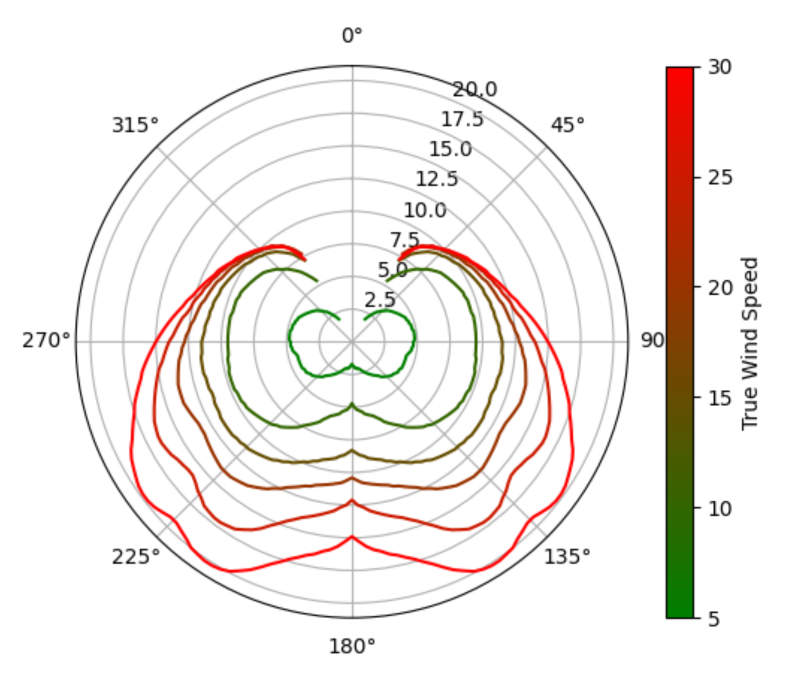
Figure 1. Example of a polar diagram as polar plot.
Applsci 12 03085 g001
Figure 2. Vector diagram showing the relations between boat direction (BD), true wind direction (TWD), true wind angle (TWA), apparent wind angle (AWA) apparent wind direction (AWD), apparent wind angle (AWA) and relative wind direction (RWD). See also page 16 in [2].
Applsci 12 03085 g002
Figure 3. How to use a polar diagram slice to obtain the boat direction (BD).
Applsci 12 03085 g003
Figure 4. An example of a rule declaring how to connect nodes by edges.
Applsci 12 03085 g004
Figure 5. An example of isochrone points with edges to trace back the optimal path.
Applsci 12 03085 g005
Figure 6. A visual representation of the hrosailing framework. Red boxes with rounded corners indicate data, yellow boxes indicate framework components. Solid arrows from multiple objects to a single indicate the possibility to compute the object at the end by using the objects at the starting points. Dashed arrows indicate the “part of” relation.
Applsci 12 03085 g006
Figure 7. Pipeline model to obtain polar diagrams (PDs) from real-world measurements.
Applsci 12 03085 g007
Figure 8. Diagram showing how to use the convex hull (gray) to obtain an overall better performance by tacks and jibes.
Applsci 12 03085 g008
Figure 9. A polar plot of the combined convex hull (dashed lines) of polar diagram slices of multiple sails (solid lines). Dashed lines corresponding to a single sail (same color) indicate manoeuvres without sail changes. Grey dashed lines indicate manoeuvres with sail changes.
Applsci 12 03085 g009
Figure 10. A visualisation of the interim results of the pipeline. Points with smaller weights are displayed with more shade (if weights are assigned).
Applsci 12 03085 g010
Figure 11. The result of the example code of Section 4.3.2.
Applsci 12 03085 g011
Figure 12. All points that can be reached from ( 42 . 5 , 43 . 5 ) in 20 min in different directions.
Applsci 12 03085 g012
Figure 13. Collected data (left) and resulting PolarDiagramCurve (right) for full sails (first row) or for foresail only (second row).
Applsci 12 03085 g013
Table 1. Table of advantages and disadvantages of different representations of polar diagrams. We use () to indicate that the corresponding feature is present to some degree.
RepresentationTablePointCloudCurve
Human usable
Human readable
Compatible with other software
Independent of interpolation()
Adaptability()
Smooth polar plot()
complete slices
adapts to real data
Publisher’s Note: MDPI stays neutral with regard to jurisdictional claims in published maps and institutional affiliations.