1. Introduction
The maturity of most giant oil fields motivates the utilization of unconventional recovery methods to increase oil production [
1]. After the primary and secondary recovery stages, enhanced oil recovery (EOR) has the potential to enable the recovery of a significant amount of oil that remains in the reservoir. EOR involves the injection of a fluid or fluids into the reservoir to supply the energy required for oil displacement. Furthermore, the injected fluids interact with the reservoir rock and formation fluid, which results in altering the physical properties of the rock and creating advantageous conditions for oil recovery [
2,
3,
4]. One of the main EOR methods applied worldwide is thermal EOR. This method supported more than 40% of total EOR production in 2015 [
5]. The mechanism of the thermal EOR method is based on reducing oil viscosity at an increased reservoir temperature. This implies that the target oil is a high-density and high-viscosity oil. Heavy oils are such an example for the target oil, and several reports on thermal EOR implementations showed that almost all of the reservoirs are heavy oil reservoirs [
6,
7,
8].
Steam huff and puff injection, also known as cyclic steam stimulation, is the method comprising cyclical steam injection into a well. After injection, the well is shut in to allow the steam to “soak” into the reservoir. The high temperature of the steam should reduce oil viscosity near the steam–oil interface. This period is called the soaking period. The well is opened again after the soaking period, producing oil at a higher rate. During the soaking period, most of the steam is condensed so the well produces both hot oil and hot water. This increase in well production performance happens because of the reduction in oil viscosity and the increase in reservoir pressure near the wellbore. After some time, the heat dissipates and oil viscosity increases. After the production declines to the pre-defined level, steam is reinjected into the well, starting a new injection/production cycle. This whole process of injection, soaking, and production is called the huff and puff method. Steam huff and puff injection is one of the most used thermal EOR methods due to its economical attractiveness and effectiveness. Furthermore, it is often used as a precursor before conducting a full field-scale steam injection. Successes in previous developed experience of this method were reported in Cold Lake Field, Canada [
9,
10], Midway Sunset Field, California [
11], Duri Field, Indonesia [
12,
13,
14] and Tia Juana Field, Venezuela [
15,
16]. In Cold Lake Field, a 100,000 cp bitumen was found and 20% of the reserves was recovered by implementing this method. In Midway Sunset Field, more than 19,000 steam cycles were performed in 1500 wells over a period of 23 years. In Duri Field, the oil production rate was increased by almost five-fold and steam huff and puff injection became a precursor to a steamflood pilot, which led to the largest steamflood implementation in the world. In Tia Juana Field, the method was applied to 145 wells and produced 30.7 million barrels of oil in 7 years.
Reservoir simulation is a crucial tool in reservoir engineering. It allows the simulation of the behavior of a dynamic reservoir model in response to the disturbance caused by the production operation. Moreover, it has become a standard in evaluating the performance of a reservoir and designing an optimized production scheme. However, despite the progress in computational hardware, the whole process of reservoir simulation remains time-consuming and expensive due to the high non-linearity of a reservoir system and the difficulty of building a reliable full reservoir model.
The cost and time inefficiency problem of reservoir simulation persists in designing a production scheme for steam huff and puff injection. Building predictive proxy models is a suitable solution to deal with this issue. A proxy model is a mathematically or statistically defined function that represents a real system or its simulation [
17]. It can provide results instantly, compared to the whole process of reservoir simulation, which incorporates screening, modeling, history matching, field development planning, and running the simulation. In reservoir engineering, proxy modeling has mainly been used for sensitivity analysis, risk analysis, history matching, production forecasting, and production optimization [
17,
18,
19,
20,
21]. Prediction of reservoir performance is considered one of the main proxy model applications. Numerous proxy models for different reservoirs under different production methods have been developed and reported in the literature. For instance, Queipo et al. [
22] developed a proxy model to optimize cumulative oil production for the steam-assisted gravity drainage method. Mohaghegh [
23] built a proxy model using a fuzzy pattern algorithm to mimic a giant oil field simulation, where the proxy model outcomes are oil and water production over time. Artificial neural network (ANN) proxy models were developed by Artun et al. [
24] for the CO
2 and N
2 cyclic injection method to predict oil production; by Sumardi and Irawan [
25] to predict coalbed methane production; by Ayala et al. [
26] to predict fluid production in gas condensate reservoir; by Sun and Ertekin [
27] in a polymer flooding process; and by Bansal et al. [
28] to forecast well production in a tight oil reservoir. Dahaghi and Mohaghegh [
29] constructed a proxy model to predict cumulative production from a fractured shale gas reservoir. Al-Mudhafar and Rao [
30] built a proxy model to predict optimum oil recovery for an immiscible gas-assisted gravity drainage method. Polizel et al. [
31] generated proxy models based on response surface methodology to predict fluid production, Net Present Value (NPV), and the recovery factor of oil. Panja et al. [
32] applied the same algorithm, comparing it to the least square support vector machine algorithm to predict hydrocarbon production from shales. Box–Behnken design was used to develop a statistical proxy model by Jaber et al. [
33] to estimate incremental oil recovery under a CO
2-water alternating gas (WAG) scheme and Ahmadi et al. [
34] to predict oil recovery in miscible CO
2 injection.
Proxy models that predict reservoir performance for steam huff and puff injection are rarely found. Attempts to develop universal proxy models for the specified case were instigated by Arpaci [
35], Sun and Ertekin [
36], and Ersahin and Ertekin [
37]. The models were presented as general models and some are the continuation and improvements from previous works over the years. Arpaci [
35] developed an expert system consisting of ANN proxy models for steam huff and puff injection with horizontal wells in a naturally fractured reservoir. The inputs of the model are reservoir rock and fluid properties, operation design parameters, and fracture design parameters. The forward models predict outputs such as the number of cycles, cycle duration, oil flowrate, and cumulative oil production. Inverse models were developed to predict operation parameters and fracture design parameters, using performance indicators such as oil production and production period as additional inputs. Most of the reservoir parameters were assumed constant, such as oil density, relative permeability, anisotropy, and capillary pressures. It was reported that the majority of testing cases had a difference in the number of cycles by two cycles, but the production prediction still falls within the acceptable error margin. Sun and Ertekin [
36] developed ANN proxy models for steam huff and puff injection. The study had the same workflow where forward and inverse models were generated as an expert system. In addition, two case studies describing examples of potential practical applications were presented. The first case study compared the performance of proxy models to the reservoir simulation result using the same inputs. The production data results showed a good agreement between the results obtained using a reservoir simulator and an artificial network model. Ersahin and Ertekin [
37] improved the Sun and Ertekin model by optimizing the generation of input data with the results focused more on the heat exchange effect around the wellbore, represented by the developed viscosity contour model.
This study aims to develop predictive models that provide reservoir performance outputs estimation for the steam huff and puff injection method. The developed predictive models are data-driven proxy models based on reservoir simulation results. These models provide improvements from the previously developed data-driven general models, where the range and distribution of the input parameters are based on the screening data of reported steam huff and puff injection field implementations. Furthermore, the provided range is comparatively wider than the previous models. As the proxy model only works within the predetermined range of input parameter values, a wider range results in higher applicability of the model to reservoir conditions that are suitable for the injection method. To the authors’ knowledge, such an investigation of implementing the screening survey data to the development of the proxy model has not been instigated. In addition, this study approaches prediction of the performance of output parameters one injection cycle at a time to achieve faster convergence when developing the model. The implemented machine learning algorithms are polynomial regression and artificial neural network, as both algorithms showed promising results in petroleum industry applications [
38,
39,
40,
41,
42]. Cumulative oil production, maximum oil rate and oil rate at the end of injection cycle are the output parameters to be modeled. These outputs address the typical production profile of huff and puff, where the production rate peaks the moment that the well is opened, then declines over a certain production period before the huff and puff cycle is repeated. Lastly, reservoir conditions that may change in one injection cycle such as pressure and water saturation are modeled to prepare the input parameters for the next cycle. The performance of multiple cycle scenarios can be determined by reinputting unchanging parameters from the previous cycle and the changing parameters that are modeled. As the models provide a quick estimation of the reservoir performance and can also be used as a sensitivity analysis and optimization tool, it is believed that the models can be of significance to engineers working in reservoir engineering and simulation.
2. Methodology
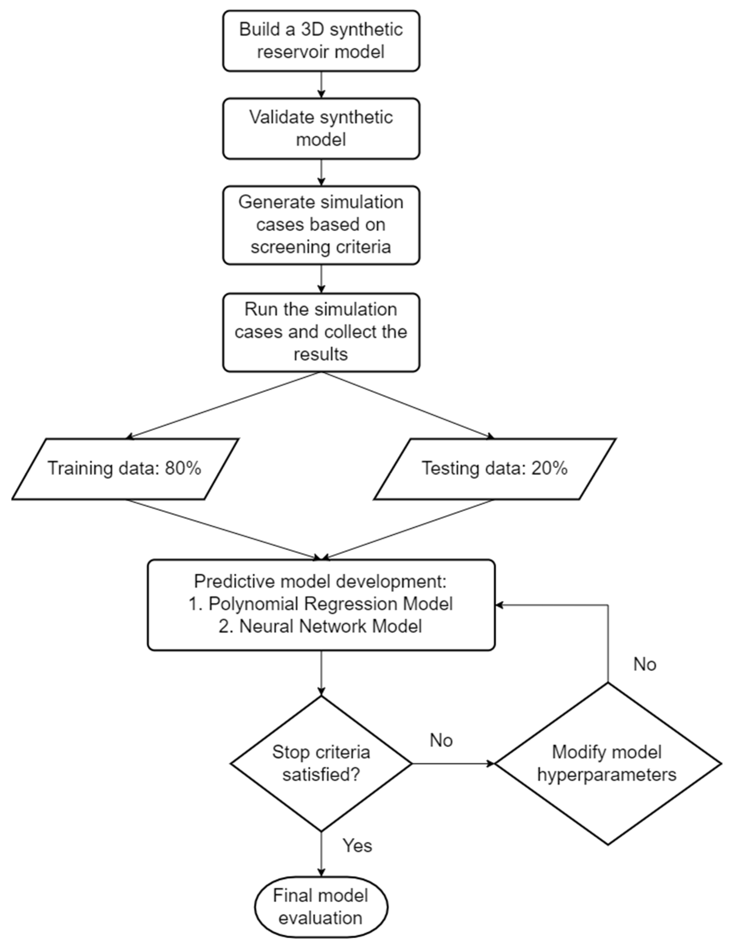
The predictive model for the steam huff and puff injection method is developed based on reservoir simulation results data using the commercial software Computer Modelling Group (CMG)
TM. The design steps are creating a synthetic reservoir model, generating simulation experimental data, and developing the predictive model. The applied methodology in this study is illustrated in
Figure 1.
2.1. Synthetic Reservoir Model
The reservoir model was developed based on the SPE 4th comparative study [
43], as illustrated in
Figure 2. It is a cylindrical grid model with 20 radial grids, 1 angular grid, and 4 vertical grids. As the huff and puff method incorporates injection, soaking and production in one well, a cylindrical geometry is preferred due to its advantage in representing the radially dominated flow around a single wellbore. The radial grid around a near-well area is refined to capture the thermal mechanism and fluid flow around the wellbore better. It has 1 well positioned at the center, which serves as both an injector and producer. All grids of the well are perforated, and reservoir properties are homogeneous for every grid.
Oil viscosity is considered as an input parameter for this model. The oil viscosity vs. temperature table was generated using Andrade’s correlation as shown in Equation (1) [
44]. Relative permeability functions were built using Corey’s equation, presented via Equation (2) to Equation (5) [
45]. The oil–water system was covered by Equations (2) and (3) and the gas–liquid system was covered by Equations (4) and (5). The variation in Corey exponents (
) covered both sandstone and carbonate rock types.
In Equation (1), is the oil viscosity, and are the Andrade viscosity constants, and is the temperature in °F. For the oil–water relative permeability system in Equations (2) and (3), is the oil relative permeability and is the water relative permeability. is the oil relative permeability at connate water saturation ; is the water relative permeability at irreducible oil saturation . is the Corey exponent for and is the Corey exponent for . For the gas–liquid relative permeability system in Equations (4) and (5), is the liquid relative permeability and is the gas relative permeability. is the liquid relative permeability at connate gas saturation and is the gas relative permeability at connate liquid saturation . is the Corey exponent for and is the Corey exponent for .
The operating parameters are steam injection rate, steam quality, steam temperature, soaking period, injection period, and production period. The initial condition of the reservoir is adjusted to be within the range of reservoir conditions of the screening criteria for steam huff and puff. Steam, with varying quality and temperature, is the injected fluid. The model simulates an injection scheme for one cycle, consisting of injection, soaking, and production periods. This thermal reservoir model is simulated using the commercial simulator CMG STARSTM.
The 3D model was then validated by comparing the results of oil production history from this model with actual field data, where the field parameters and results used are from the Midway Sunset field [
46].
Figure 3 shows the history matching of oil production rate from this simulation model to the field data, which expressed good agreement. Furthermore, the cumulative oil production result from this model is 878 m
3, in comparison to field data, which is 888 m
3. This suggests that they are in good agreement with each other. It can be inferred that the synthetic model is valid and applicable for further simulation studies.
2.2. Generation of Simulation Experimental Data
Simulation experiment cases were generated by varying the values of 28 input parameters within a provided range. They were designed using the Latin Hypercube Method, where this method has an advantage over classic experimental design in orthogonality and space-filling, resulting in a unique input parameter value for each simulation case [
47]. The range of each parameter is determined from the screening criteria of steam huff and puff applications obtained from the literature study. A study from Hama et al. [
48] provided the screening criteria in which a data cleaning process had been conducted to remove outliers and duplicates from the database. Furthermore, the distribution of each screening parameter was determined and used in this study to generate the experimental cases. The range of input parameter values of Corey’s equations was selected to satisfy practical fluid flow conditions and accommodate the different pore size distributions of sandstone rock. Combining these with the former screening criteria by Ali [
49] and Taber et al. [
50], the list of input parameters with their range for this study was determined and is presented in
Table 1.
A sampling control was conducted before running the simulation to avoid unrealistic experiment cases, which result in reservoir models that physically do not exist. Combinations of input parameters needed to be controlled, such as oil density, reservoir pressure and temperature, porosity–permeability, rock–fluid properties, and drainage area. After sampling control, 6304 simulation experiment cases were ready to be simulated using a reservoir simulator. The reservoir performance of steam huff and puff injection was represented in cumulative oil production, maximum oil rate per cycle, and the oil rate at the end of the cycle. Multiple cycle injection performance can be estimated by re-inputting parameters into the proxy model, as well as the input parameter that may have changed after conducting the previous huff and puff cycle. The input parameters that may have changed and were modeled in this study are reservoir pressure, reservoir temperature, and water saturation in the reservoir. All of the outputs from each simulation result are captured as a response variable to build the predictive model.
2.3. Predictive Model Development
The CMG CMOSTTM module was utilized to develop the predictive model. This module was employed to run the generated simulation cases, record the output target results and alter the hyperparameters to build the predictive model. From 6304 simulation data, 80% of the result was treated as training data and the remaining 20% was treated as testing data. In this study, polynomial regression and artificial neural network models were developed.
The polynomial regression (PR) method is a form of analysis to determine the relationship between input variables and response variables as a polynomial equation. The general quadratic polynomial regression is presented in Equation (6) below:
where
are the coefficients of linear (
) terms,
is the coefficient of quadratic (
) terms, and
is the coefficient of the interaction (
) terms. All coefficients are determined by using the least-squares method.
It is common that some of the terms in the model are not statistically significant. The model can be improved by removing statistically insignificant terms, which can be determined by evaluating the significance probability. As the insignificant variables are reduced, the modified model is often named a reduced polynomial regression model. In this study, the reservoir performance outputs are represented as a reduced quadratic function of the 28 input parameters.
Artificial neural network (ANN) is a model that emulates the biological neural system. It consists of nodes that are similar to neurons in the human brain. A node receives signals from adjacent nodes and processes them to produce an output. The ANN model structure is presented in
Figure 4. It consists of an input layer, an output layer, and one or multiple hidden layers in between. Each neuron from a layer is connected to the neurons from other nearby layers with a connection called weight, which represents an influence of corresponding input on the connected neuron. Then, to transfer the contained information, an activation (or transfer) function is used. This is also known as forward propagation and it is conducted for every connection in the network. After defining the model, the back propagation algorithm is used to readjust the weight and minimize the error between the output and the database. In this study, a multilayer neural network structure was implemented, where the input layer consisted of 28 neurons as input parameters (listed in
Table 1), the output layer consisted of 1 neuron as output parameter, and there were multiple hidden layers in between, with each hidden layer consisting of a number of neurons. The activation function for all layers is the hyperbolic tangent function (tanh) presented in Equation (7). This activation function is used as it shows good performance when employed to build a multilayer neural network.
Three evaluation metrics were employed to assess the performance of the developed models, which were the coefficient of determination (R-square), the mean absolute error (
MAE) and root mean square error (
RMSE). The R-square is a statistical metric used to measure the regression prediction compared with the actual data point, where 1 indicates a perfect fit. The adjusted R-square is a modification of the R-square calculation, where it takes into account the number of input parameters
. Its value is always lower than the R-square. Both are presented in Equations (8) and (9), respectively, where
is the predicted value,
is the simulation data, and
is the number of experimental cases. In this study, the adjusted R-square will be used as the evaluation metric for the fitting coefficient, as it has the potential to be more accurate for a high number of input parameters. A scatter plot of simulated and predicted data is presented to visualize the performance of the model. In a good, representative model, both training and testing data points should be located close to the 45-degree baseline
, as the baseline represents a perfect fit (
). Additionally, the
MAE and
RMSE are calculated for the training and testing results of each model.
MAE is the average difference of the predicted and actual data, which indicates the relative deviation between them.
RMSE is the square root of the mean of the square of all of the errors. It gives a relatively high weight to large errors and grows as the frequency of large errors increases. Both metrics can range from 0 to infinity and lower values are preferred. The
MAE and
RMSE are given in Equations (10) and (11), respectively.
Lastly, Sobol analysis [
51], a variance-based sensitivity analysis, was conducted for each developed proxy model to determine the significance of input parameters toward each model. This method aims to quantify the amount of variance that each input parameter contributes to the variance of output. It identifies the total effect of an input parameter, which can be separated into main effect and interaction effect [
52]. The main effect is the contribution to model output variance based on the variation of the input parameter itself and the interaction effect is the contribution of particular combinations of model input. The sum of both main and interaction effects is called the total effect. This analysis is conducted for the model that has the better performance after evaluating the fitting metrics between the polynomial regression and the neural network model.
3. Results and Discussion
Each of the proxy models is represented as a function of 28 input parameters and evaluated based on the R-square value. The predicted and simulated data points should be scattered close to the baseline, as it represents the best fit for the model. In the polynomial model, as shown in Equation (6), the least-square fitting algorithm was carried out to determine the coefficients of all terms. The form of the equation is an output parameter as a function of input parameters. In the neural network model, the number of layers and neurons in each layer are pre-assigned before training the model. The end result is a table that contains weight values for all node connections. Through trial-and-error, the hyperparameters of all the developed models were optimized to achieve a high prediction performance.
3.1. Proxy Models for Predicting Reservoir Performance
The reservoir performance outputs are represented by cumulative oil production, maximum oil rate per cycle, and oil rate at the end of the cycle. As mentioned above, these outputs address the typical production profile of huff and puff. Predicted and simulated data points for each output are presented in
Figure 5,
Figure 6,
Figure 7,
Figure 8,
Figure 9 and
Figure 10, respectively. Overall, the neural network model provides a better fit for training and testing data when compared to the polynomial regression model.
The cumulative oil production () values range from 0.1 to 100 MSTB. The polynomial model is the equation of the output as a function of all input parameters. The neural network model of is a deep neural network with multiple hidden layers, which has an architecture of the following: 1 input layer with 28 input neurons, 1 output layer with 1 output neuron, and five hidden layers with an 8–8–6–4–4 neuron configuration. The input and output layer configurations are the same for all neural network models mentioned in this study. For training data, the R-square for the polynomial regression model and the neural network model are 0.755 and 0.981, while the R-square for the testing data is 0.735 and 0.959. The MAE of the training and testing data for the polynomial regression model is 7.53 Mbbl and 8.28 Mbbl, and for the neural network model, this is 1.39 Mbbl and 1.76 Mbbl. The RMSE of the training and testing data for the polynomial regression model is 10.39 Mbbl and 11.65 Mbbl and, for the neural network model, 2.31 Mbbl and 3.36 Mbbl. The neural network model presents a better result than the polynomial regression model. The prediction for the training data is mainly good where points are around the baseline. The prediction in testing data is well below the 20 Mbbl and starts to scatter further from the best fit curve. The simulation results showed around 90% of the cumulative production data are below 20 Mbbl, thus making the prediction better inside that interval. It can also be observed that the polynomial regression model predicts negative values while the neural network model does not, which shows the advantage of the neural network model over the polynomial model as negative production values do not exist in reality.
The maximum oil rate (
) values range from 0 to 2000 stb/d. The polynomial model is the equation of the
output as a function of all input parameters. The neural network model of
has an architecture of five hidden layers with an 8–8–6–4–4 neuron configuration. For the training data, the R-square for the polynomial regression model and the neural network model are 0.706 and 0.957, while the R-square for the testing data is 0.675 and 0.931. The MAE of the training and testing data for the polynomial regression model is 221.6 bbl/d and 239.9 bbl/d and, for the neural network model, 63.4 bbl/d and 74.3 bbl/d. The RMSE of the training and testing data for the polynomial regression model is 281.5 bbl/d and 303.6 bbl/d and, for the neural network model, 97.6 bbl/d and 126.4 bbl/d. It can be seen from
Figure 7 and
Figure 8 that the neural network model far outperforms the polynomial regression model. The training and testing data in the neural network are generally clustered around the best fit curve, with the prediction for both being well below 250 bbl/d.
The oil rate values at the end of the cycle (
) range from 0 to 400 stb/d. The polynomial model is the equation of the
output as a function of all input parameters. The neural network model of
has an architecture of five hidden layers with an 8–8–6–4–4 neuron configuration. For training data, the R-square values for the polynomial regression model and the neural network model are 0.561 and 0.953, while the R-square for the testing data is 0.524 and 0.847. The MAE of the training and testing data for the polynomial regression model is 29.1 bbl/d and 31.1 bbl/d and, for the neural network model, 8.6 bbl/d and 11.8 bbl/d. The RMSE of the training and testing data for the polynomial regression model is 43.0 bbl/d and 45.9 bbl/d and, for the neural network model, 14.1 bbl/d and 21.7 bbl/d. The polynomial regression model performs poorly in comparison to the neural network model in this output model, as shown in
Figure 9 and
Figure 10. Though the deviation is noticeable, overall, the data points for training and testing data have a good correlation to the best fit curve. The prediction for both the training and testing data is below the 20 bbl/d and started to drift further from the best fit curve. The data results show that around 80% of the data points are below 20 bbl/d, making the prediction better inside that interval.
Sobol analysis is implemented for the neural network models to observe the significance of input parameters.
Table 2 presents 10 input parameters that provide the highest contribution towards predicting the output for the set of base input parameters described in
Table 1. In general, reservoir water saturation, represented by Sw, and oil viscosity, represented by Andrade’s viscosity constant ViscB, are the two parameters with the highest impact on the reservoir production performance models of steam huff and puff injection. The contributions of Sw and ViscB to the
model are 16.5% and 11.0%; for the
model, 53.1% and 25.5%; and for the
model, 10.7% and 12.0%.
Reservoir water saturation is directly related to the volume of oil inside the reservoir, hence the change in its value impacts the amount of oil production. The oil viscosity is a determining factor of oil production performance, as the objective of steam huff and puff injection is to lower the oil viscosity, allowing easier flow of the oil and increasing production. A higher initial oil viscosity will result in less efficient production for a fixed amount of steam injection due to the higher need for heat energy to decrease the viscosity. It is worth mentioning that porosity is not on the list for and proxy models, and appears only in the lower part of the list of the model, despite its significance as a reservoir rock property that also directly links to the volume of oil reserve. This can be explained by observing the distribution of porosity input values from the screening data from the field implementation report, where a large number of porosity values might be clustered on a small range due to a skewed distribution. In addition, the presence of other volume-related parameters with possibly wider distribution input values further increases the dominance of the contribution towards the proxy model outputs, such as water saturation and drainage area, which are observed in the list.
The other affecting parameters for each proxy model can be seen in the table, though their contributions are significantly lower compared to the first two parameters. For the model, reservoir pressure and the bulk volume of the reservoir are the next contributors to the model. For the model, these are reservoir pressure and permeability; and for the model, the production period of the steam huff and puff cycle, reservoir pressure, and the drainage area of the well.
3.2. Proxy Models for Predicting Reservoir Conditions after an Injection Cycle
The reservoir condition outputs after one cycle are represented by reservoir pressure, reservoir temperature, and reservoir water saturation. These outputs address the reservoir parameters that are most likely to change in one injection cycle. The parameters are defined as the average parameter value in the reservoir model, assuming that the effect of steam injection has mostly diminished and a new injection cycle can be started in the reservoir. Predicted and simulated data points for each output are presented in
Figure 11,
Figure 12,
Figure 13,
Figure 14,
Figure 15 and
Figure 16.
The reservoir pressure values at the end of the injection cycle (
) from the results dataset range from 0 to 1200 psi. The polynomial model is the equation of the
output as a function of all input parameters. The neural network model of
has an architecture of three hidden layers with a 10–8–6 neuron configuration. For the training data, the R-square for the polynomial regression model and the neural network model is 0.878 and 0.991, while the R-square for the testing data is 0.877 and 0.989. The MAE of the training and testing data for the polynomial regression model is 64.8 psi and 66 psi and, for the neural network model, 14.9 psi and 16.1 psi. The RMSE of the training and testing data for the polynomial regression model is 85.8 psi and 87.6 psi and, for the neural network model, 22.3 psi and 25.5 psi. It can be seen in
Figure 11 and
Figure 12 that the neural network model performs better than the polynomial regression model. The training and testing data in the neural network are generally clustered around the best fit curve. It is also worth highlighting that the neural network model predicted no negative values, in comparison to the polynomial regression model that yields some negative data points.
The reservoir temperature values at the end of the injection cycle () from the results dataset range from 50 to 194 °F. The polynomial model is the equation of the output as a function of all input parameters. The neural network model of has an architecture of three hidden layers with an 8–6–4 neuron configuration. For training data, the R-square for the polynomial regression model and the neural network model is 0.962 and 0.995, while the R-square for the testing data is 0.954 and 0.978. The MAE of the training and testing data for the polynomial regression model is 2.5 °F and 2.6 °F and, for the neural network model, is 0.9 °F and 1.3 °F. The RMSE of the training and testing data for the polynomial regression model is 3.8 °F and 4.2 °F and, for the neural network model, is 1.4 °F and 2.9 °F. The performance between the two models does not differ much, though it can be seen that some training data points drift away in the prediction–simulation plot of the polynomial regression model. Overall, the training and testing data in the neural network fit well around the best fit curve.
The reservoir water saturation values at the end of the injection cycle () from the results dataset range from 0 to 0.88. The polynomial model is the equation of the output as a function of all input parameters. The neural network model of has an architecture of three hidden layers with a 4–4–2 neuron configuration. For training data, the R-square values for the polynomial regression model and the neural network model are 0.939 and 0.982, while the R-square values for the testing data are 0.935 and 0.980. The MAE of the training and testing data for the polynomial regression model is 0.0259 and 0.0264 and, for the neural network model, is 0.0152 and 0.0156. The RMSE of the training and testing data for the polynomial regression model is 0.0331 and 0.0338 and, for the neural network model, is 0.0208 and 0.0218. Similar to the reservoir temperature model, polynomial regression and the neural network model are observed fit well. For the polynomial model, a slight distortion is detected above the 0.6 water saturation value.
After conducting Sobol analysis for these models, it is observed that the parameter that dominates the contribution to each output model is the initial value of the parameters themselves, before implementing the steam huff and puff injection cycle.
Table 3 shows the top five highest contributing parameters, as the other parameters contribute significantly less than the first five parameters. The most important parameter for the reservoir pressure model at the end of the cycle is the initial pressure with 32.7%. For the reservoir temperature, the most important parameter is the initial temperature with 50.9% significance and for reservoir water saturation is the initial water saturation with 78.5% significance. This explains the high fitting value of both the polynomial regression model and the neural network model, where the model is highly linear due to the dominance of one input parameter. This proposes the idea that at the end of the cycle, the traces and effects of steam injection have diminished, leaving the reservoir condition to be nearly similar to the initial condition of the reservoir that demanded the steam injection treatment. However, for the reservoir pressure model, water saturation and viscosity are other parameters that provide a significant contribution. This result can be justified considering that reservoir pressure changes as the volume of the fluid filling the pore spaces changes. Production activity, which displaces the fluid out from the reservoir, depletes the reservoir pressure. This process is the underlying mechanism that determines the reservoir production performance. Hence, the two most important parameters from the developed production predictive models above—water saturation and oil viscosity—may possibly take part in impacting the reservoir pressure model.
3.3. Evaluation of Model Fitting and Performance Metrics
A summary of evaluation metrics for each proxy model is presented in
Table 4 and
Table 5. It can be seen that, in general, the performance of the neural network models is optimum compared to the polynomial regression models. This is due to the nature of both models, where the high nonlinearity presented in this modeling problem is well captured by the neural network model compared to the polynomial regression model. For training and testing data of the neural network model, almost all of the R-square values are above 0.9, which shows a good fit. Additionally, the MAE and RMSE values are notably lower than the polynomial models. A good agreement between the fitting indicator of training and testing data indicates that the model is not overfitting. Overfitting in a model is undesirable, as that implies that the model only remembers the training data and may perform poorly when exposed to unseen test data. This is considered when designing the experiment cases, where the combination of input parameter values is unique for each case.
The observations from the prediction and simulated plot demonstrate that deviations in testing data points are seen past a certain threshold for each neural network model—for instance, above 20 Mbbl values in the testing data for the model. As mentioned previously, any deviation past this value may occur as a result of the imbalanced proportion of data points along the output interval. After running the simulation, the cumulative oil production data below 20 Mbbl are around 90% of the results. This leads to fewer data being provided into the model above that threshold, affecting the model’s accuracy. The same can be expressed for the model, where the testing data points drift significantly past the 20 bbl/day threshold, resulting in a relatively lower R-square value in comparison to the other neural network models. Inversely, it can be inferred that the prediction performance for results below that threshold is excellent. For this specific model, possible improvement can be applied through creating separate proxy models for low and high values of based on that threshold, which will include re-evaluating input values and their distributions that result in low and high predictions.
The neural network models presented in this study can be applied for accurately determining reservoir performance in steam huff and puff injection. These predictive models save a large amount of time and costs and are believed to be helpful in assisting users for designing simulation scenarios. It is worth noting the limitation of the proxy model that it is only applicable as long as the input parameter values are within the parameter intervals of the model. The workflow used in this study can be applied for developing proxy models of other reservoir configurations or injection method variations; for example, in a fractured reservoir or a chemical-assisted steam huff and puff injection.


