1. Introduction
Energy and environment are the focal points attracting the attention of the international community due to the depletion of fossil fuels and the increasing emissions of carbon dioxide [
1,
2]. Hydrogen (H
2) is considered to be a promising energy carrier of sustainable clean energy in the 21st century. The proton exchange membrane fuel cells (PEMFC) system can transform the chemical energy of H
2 into electricity directly, and the by-products during the electrochemical process are heat and water [
3,
4]. It is a promising power conversion device because of its satisfactory characteristics except for the high cost and limited lifetime. Predicting the lifetime of the PEMFC system can help the users to take action in advance to extend its working life.
Model-based and data-driven methods are two typical classifications of existing lifetime prediction methods [
5,
6]. Data-driven methods, which are mainly based on machine learning (ML) theory, construct the nonlinear degradation relations [
7,
8]. One of the patterns of ML, the recurrent neural network (RNN), has shown great power in nonlinear time series prediction. Nevertheless, the RNN has some weaknesses such as slow convergence rate and the existence of bifurcation. To overcome the weaknesses of RNN, the echo state network (ESN) was proposed by Prof. Jaeger et al. in [
9]. There are two characteristics of ESN: one is a large, randomly generated reservoir that is used to replace the hidden layers of RNN; the other is the weight matrices (input and internal) that are generated randomly. The ESN has a faster convergence rate and lower computational training cost than the traditional RNN. Nevertheless, the hyperparameters of ESN (leaking rate, spectral radius, regularization coefficient, reservoir neuron number, reservoir connectivity, etc.) need to be carefully tuned from human expertise [
10].
For the PEMFC system’s lifetime prediction application, the ESN has first been applied in [
11] to estimate the steady-state cell voltage by the single-step ahead prediction pattern. Four kinds of reservoirs are compared in [
12], and the delay line reservoir (DLR) and the simple cycle reservoir (SCR) have the best precision values. A cycle reservoir with a jump (CRJ) model has been proposed in [
13], and this structure is validated on the steady-state datasets. The CRJ model can speed up the linear fitting process and improve prediction accuracy. In ref. [
14], the steady-state cell voltages are divided into the approximation part and detail part by wavelet transform, and then double ESNs with different dynamic characteristics are utilized to deal with the voltage signal separately. This double ESN structure could improve prediction accuracy. The hyperparameters of ESN in [
11,
12,
13,
14] are set by the trial-and-error method. Inspired by the separation concept in [
14], the wavelet transform and multiple ESNs are proposed in [
15] to deal with the multi-timescale degradation features under the dynamic operating conditions in the long-term prediction horizon. In ref. [
15], the hyperparameters of the spectral radius and leaking rate are optimized by the grid-search method, and the prediction accuracy has been improved. To improve the prediction efficiency, the original degradation data prediction is replaced by the shortened coefficients in the discrete wavelet transform process [
16]. The prediction data points can be shortened by a factor of 8, and the hyperparameters of ESN (spectral radius, leaking rate, and regularization coefficient) are optimized by the genetic algorithms (GA) method. In ref. [
17], the analysis of variance (ANOVA) method is applied to analyze the four hyperparameters of the reservoir neuron number, reservoir connectivity, spectral radius, and leaking rate under the steady-state dataset. Results show that the spectral radius has the biggest effects on the prediction performance. Additionally, based on the ANOVA method, the effects of three hyperparameters (i.e., leaking rate, spectral radius, and regularization coefficient) have been analyzed under the dynamic operating conditions [
18]. Results show that the interaction of the spectral radius and regularization parameter has the biggest effect, and the effects of the spectral radius rank second.
Based on the ANOVA analysis results of [
17], a multi-reservoir ESN structure is proposed in [
19], and each reservoir has a different spectral radius. This multi-reservoir ESN can avoid the optimization of the spectral radius, and its effectiveness is validated under the steady-state cell voltage prediction condition. As an extension of the work in [
19], the ESN and Markov chains are combined to predict the cell voltage under the dynamic micro-combined heat and power (
μ-CHP) load profile [
20]. The RUL prediction by the combined structure can be realized with a mean relative accuracy below 17%. An ensemble ESN network has recently been proposed to avoid hyperparameter optimization and improve the adaptiveness of lifetime prediction [
21]. A dynamic health indicator of “virtual steady-state voltage (VSV)” is proposed based on linear parameter varying (LPV) models. Then, a number of ESNs with different combinations of hyperparameters (leaking rate and spectral radius) are used for the VSV prediction. Finally, the long-term RUL prediction and a confidence interval of 95% confidence level are given in detail. In the past two years, the multi-input ESN structure is proposed to improve the prediction accuracy of the RUL [
18,
22,
23,
24]. The effects of the operating parameters (i.e., current, temperature, and pressure) are fully analyzed under the steady-state and dynamic operating conditions in [
18,
22] separately. The multi-input ESN structure could improve the prediction accuracy regarding the health indicator and the scheduled current as the double inputs are more meaningful in practice. In ref. [
23], the ambient temperature and stack voltage are used as the double inputs of ESN to improve the RUL prediction accuracy. The normalized root mean square error is equal to 0.098 with a prediction over 2000 h. In ref. [
24], the input parameters of ESN are evaluated and selected by the least absolute shrinkage and selection operator (LASSO), and then the degradation-related parameters are used for the RUL prediction. Results show that the ESN with eight input parameters is the optimal choice. Both [
23] and [
24] are validated by the steady-state datasets.
In the current state-of-art, the developments of ESN for the PEMFC system’s lifetime prediction are focused on the ESN structure (reservoir forms, ensemble ESN, multi-input ESN, etc.) and hyperparameter optimization. In the practical implementation process of ESN, the input and internal weight matrices (
Win and
W) remain unchanged after they have been drawn from a random distribution. Nevertheless, the effects of the distribution shape of
Win and
W on the lifetime prediction accuracy have not been reported yet. There is abundant evidence that the ensemble structure can improve the prediction robustness and stability such as the ensemble neural network model [
25], particle filtering [
26], and extreme learning machine [
27]. The ensemble ESN is proposed in [
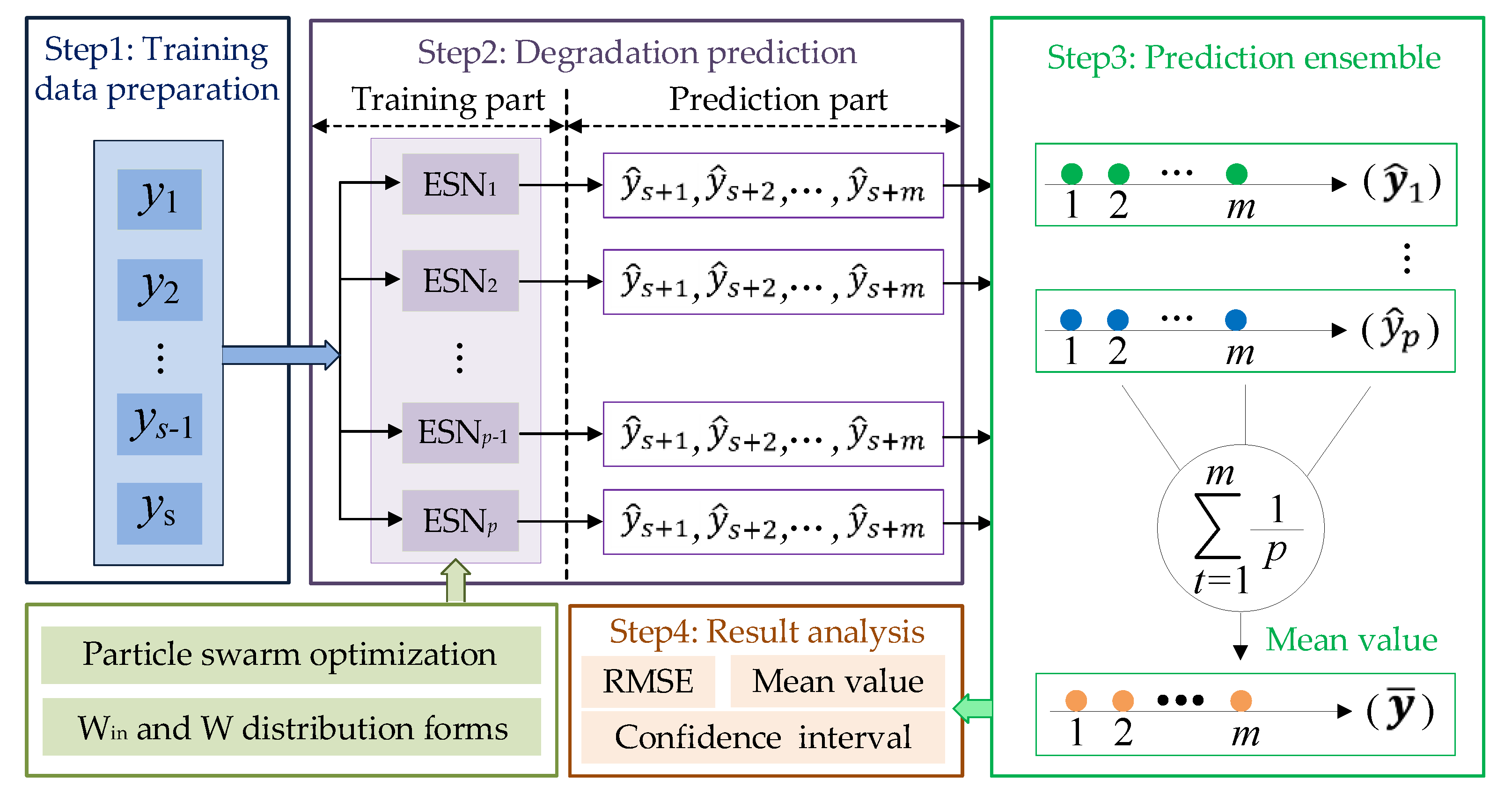
21], and the effects of the leaking rate and spectral radius have been fully analyzed. Nevertheless, the statistical property of the ESN, e.g., the uncertainty caused by the random matrices, has not been analyzed yet. Based on these two motivations, the contributions of this paper are summarized as follows:
The effects of two distribution shapes (uniform and Gaussian distribution) of Win and W on the prediction accuracy are explored;
The metaheuristic technique of particle swarm optimization (PSO) is utilized to optimize the hyperparameters of the leaking rate, spectral radius, and regularization coefficient;
The uncertainty of the ensemble ESN caused by the random matrices is statistically analyzed under three different operating conditions.
3. Experimental Results
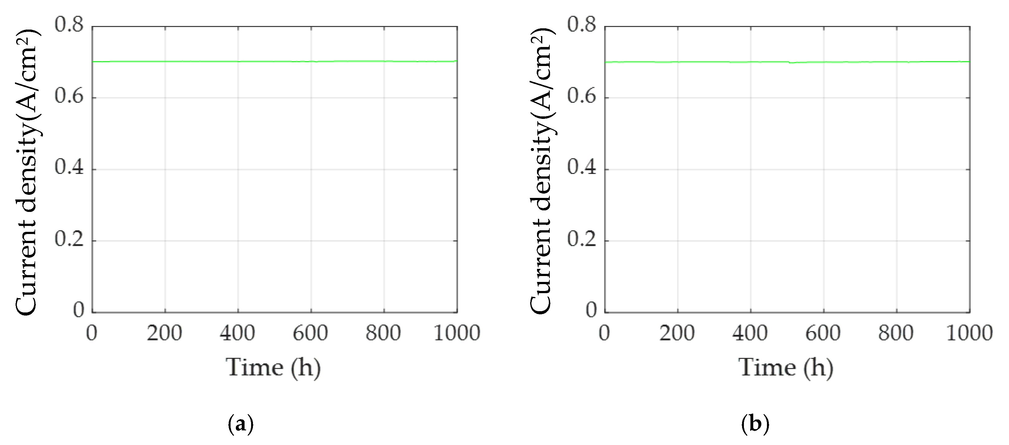
Three degradation datasets under different operation conditions are used for exploring the prediction effects of two distribution shapes of weight matrices, testing the performance improvements of the ensemble ESN, and statistically analyzing the uncertainty of random matrices. The steady-state and quasi-dynamic datasets come from the open data of the 2014 Prognostic and Health Management Data Challenge [
22]. Two PEMFC stacks are used for the 1000 h duration test under the steady-state and quasi-dynamic operating conditions. There are 5 cells for both stacks, and their active area is 100 cm
2, the operating temperature is 80
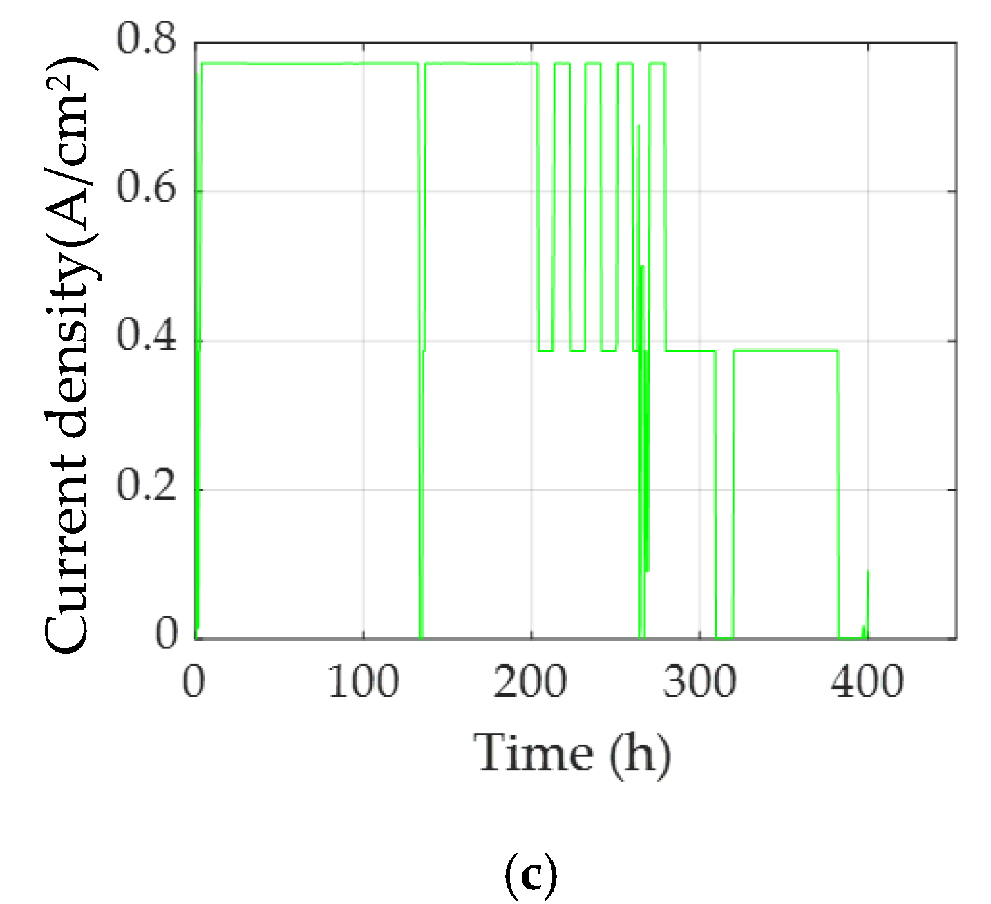
, and the back pressure is 0.2 MPa. For the steady-state test, the constant current is 70 A. For the quasi-dynamic test, the current ripples (7 A) at different frequencies (from 50 mHz to 10 kHz) are superimposed to the constant current (70 A) for the electrochemical impedance spectroscopy (EIS) measurement. The third dataset comes from a PEMFC stack for 382 hours’ duration test under the dynamic
μ-CHP load profile. The current has a cycle between 170 A and 85 A. The stack consists of 8 cells, and the active area is 220 cm
2, the operating temperature is 80
, and the back pressure is 0.15 MPa [
18]. The load profiles of the three tests are shown in
Figure 3.
3.1. Steady-State Operating Condition
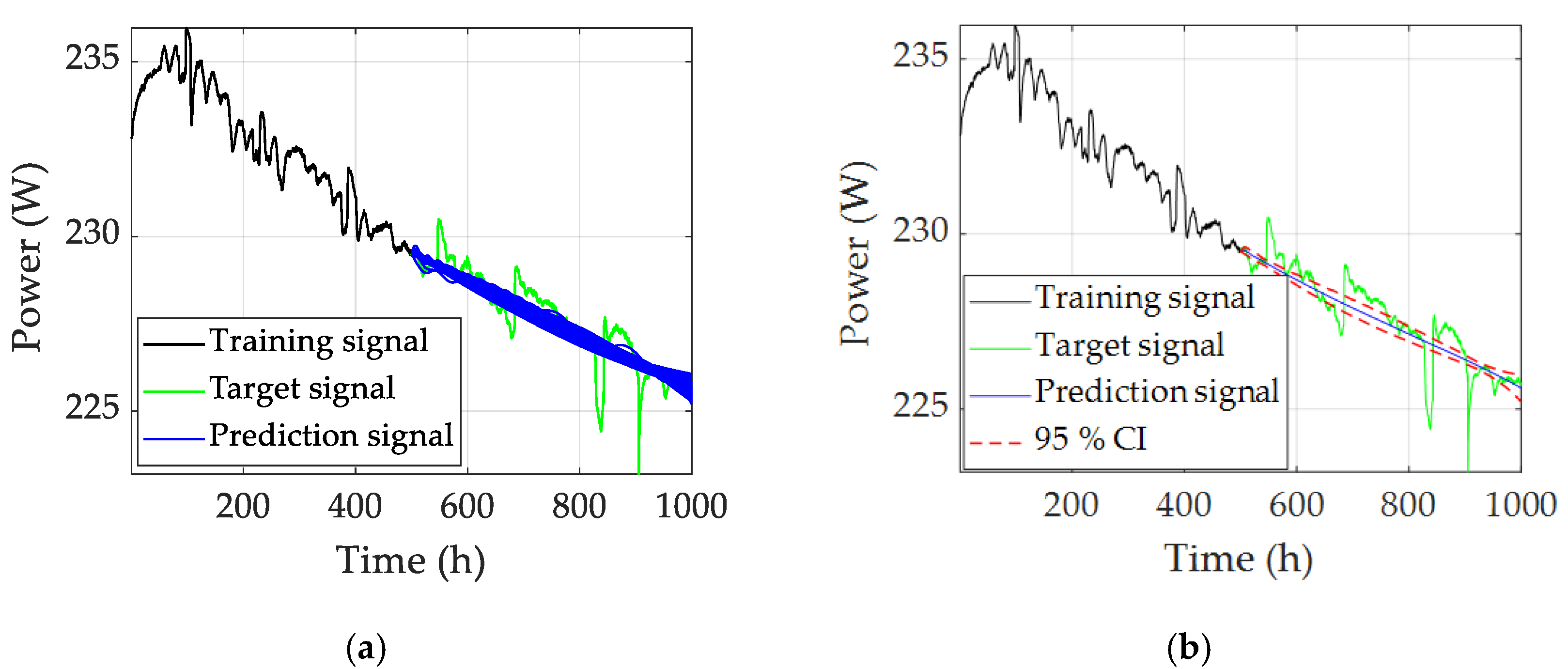
In the steady-state operating condition, the stack output power is used as the degradation health indicator. Half of the data (0–500 h) is used for training the ESN, and the rest of the data (501–1000 h) is used for prediction. During the prediction procedure, 100 individual ESNs have 100 groups of prediction results. Then, the mean value, variance, and 95% CI of the predicted results can be calculated at each time step. When
Win and
W follow the uniform distribution, the RUL prediction results are shown in
Figure 4. Taking the first 10 groups of ESNs as an example, their hyperparameters and RMSE are shown in
Table 1.
After changing the distribution shapes of
Win and
W to Gaussian distribution, the RUL prediction results under the steady-state operating condition are shown in
Figure 5. The hyperparameters and RMSE of the first 10 groups of ESNs are shown in
Table 2. To analyze the effects of the two matrices’ distribution shapes of
Win and
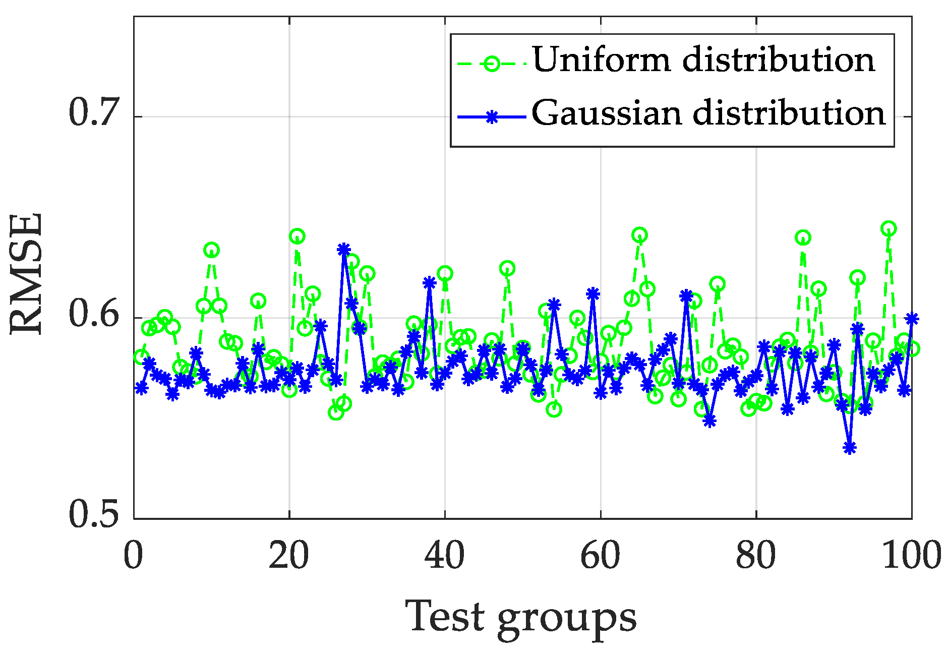
W on the prediction accuracy, the RMSE of 100 ESNs is shown in
Figure 6.
The average RMSE under the Gaussian distribution (0.57488) is lower than the average RMSE under the uniform distribution (0.58602) for the steady-state test. The mean prediction results of the ensemble ESN are calculated, i.e., 0.57841 for uniform distribution and 0.56966 for Gaussian distribution.
3.2. Quasi-Dynamic Operating Condition
In the quasi-dynamic operating condition, the stack output power is used as the degradation-related health indicator. Similar to the steady-state operating condition, half of the data (0–500 h) is used for training the ESN, and the rest of the data (501–1000 h) is used for prediction. When
Win and
W follow the uniform distribution, the RUL prediction results are shown in
Figure 7. Taking the first 10 groups of ESNs as an example, their hyperparameters and RMSE are shown in
Table 3.
After changing the distribution shapes of
Win and
W to Gaussian distribution, the RUL prediction results under the quasi-dynamic operating condition are shown in
Figure 8. The hyperparameters and RMSE of the first 10 groups of ESNs are shown in
Table 4.
To analyze the effects of the two matrices’ distribution shapes of
Win and
W on the prediction accuracy, the RMSE of 100 groups of ESNs is shown in
Figure 9. The average RMSE under the Gaussian distribution (1.19634) is lower than the average RMSE under the uniform distribution (1.27562) for the quasi-dynamic test. The mean prediction results of the ensemble ESN are calculated, i.e., 0.95657 for uniform distribution and 0.90618 for Gaussian distribution.
3.3. Dynamic Operating Condition
In the dynamic operating condition, the RPLR is used as the degradation health indicator, which has been described in detail in our previous work [
18]. First, the polarization curve of the PEMFC stack at the beginning of life (BoL) is measured. The BoL power at different currents can be calculated to form a table. Secondly, the power at time step
t can be calculated by the measured current (
It) and voltage (
Ut). Finally, the RPLR at time step
t is calculated by
where
Pt is the power at time step
t and
P0 is the BoL power, which is determined by the look-up table method. The
Pt and
P0 are at the same current level.
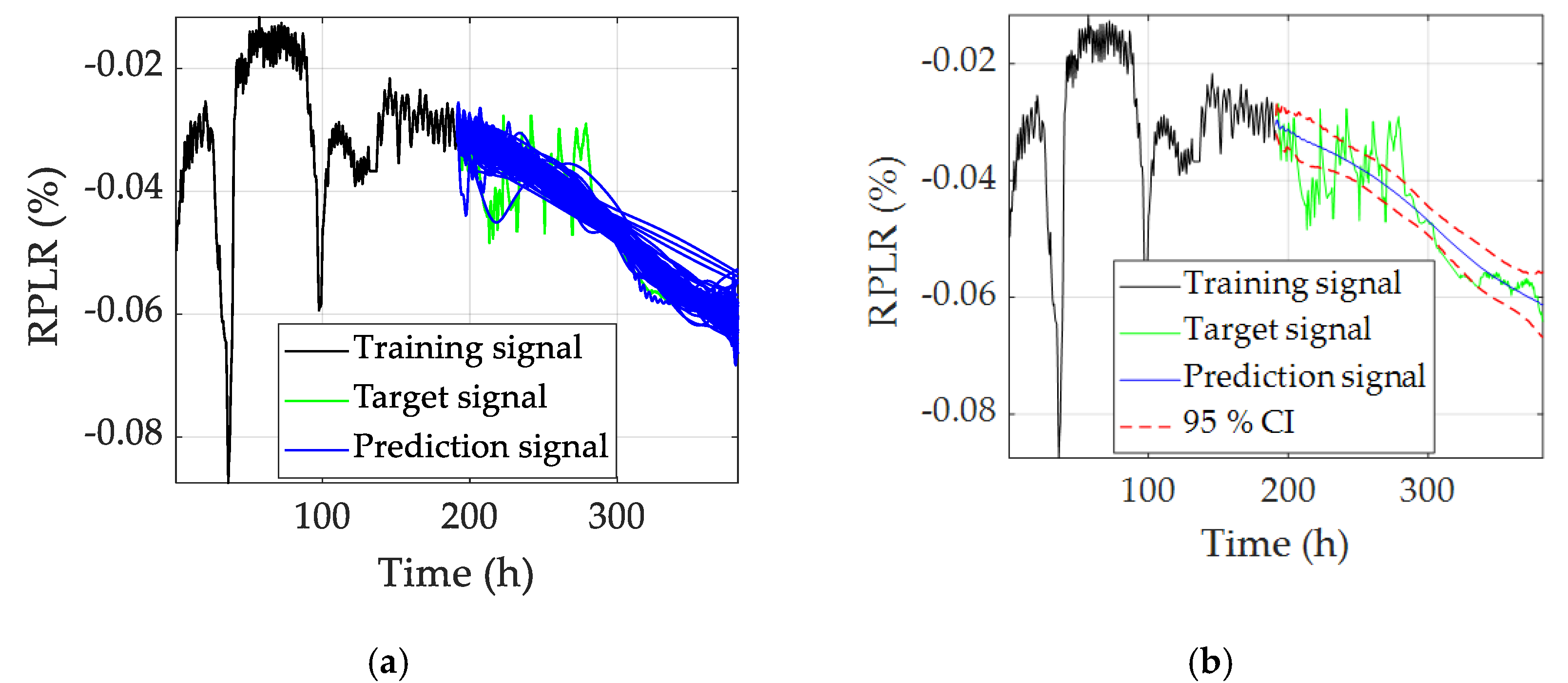
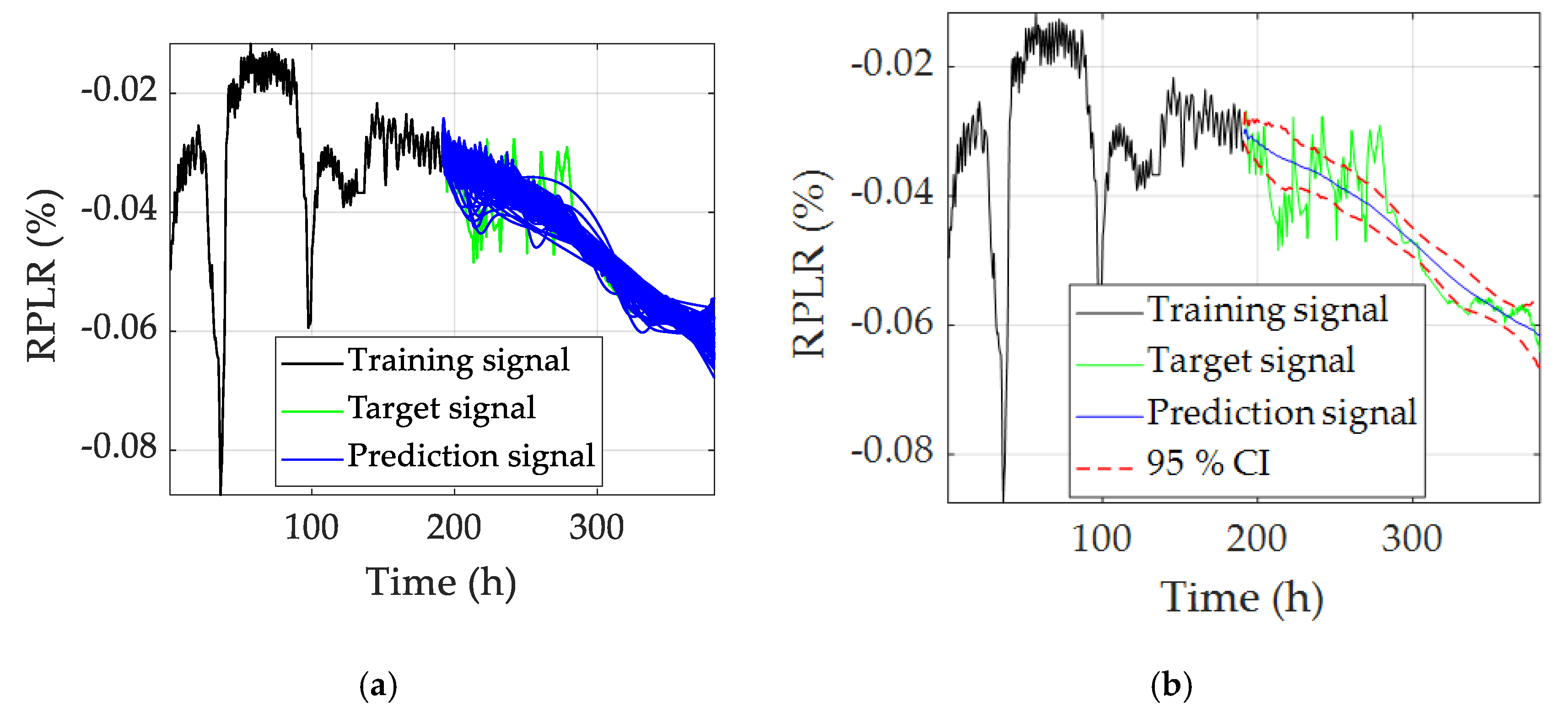
Half of the data (0–191 h) is used for training the ESN, and the rest of the data (192–382 h) is used for prediction. When
Win and
W follow the uniform distribution, the RUL prediction results are shown in
Figure 10. Taking the first 10 groups of ESNs as an example, their hyperparameters and RMSE are shown in
Table 5.
After changing the distribution shapes of
Win and
W to Gaussian distribution, the RUL prediction results under the dynamic operating condition are shown in
Figure 11. The hyperparameters and RMSE of the first 10 groups of ESNs are shown in
Table 6.
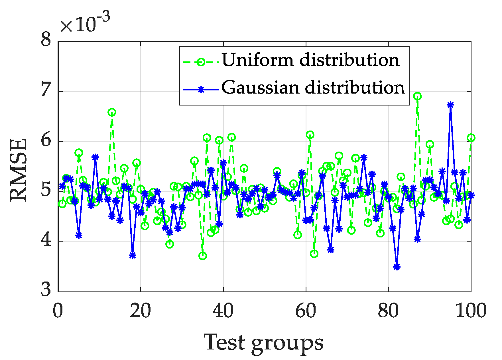
The RMSE of 100 groups of ESNs is shown in
Figure 12. The average RMSE under the Gaussian distribution (0.00489) is lower than the average RMSE under the uniform distribution (0.00502) for the dynamic test. The mean prediction results of the ensemble ESN are calculated, i.e., 0.00473 for uniform distribution and 0.00464 for Gaussian distribution.
Among these three different operating conditions, each random generation of Win and W produces a different prediction result. The essential reason is that the randomness of the matrices changes the weight values of the connected neurons, and the random weight leads to different neuron behaviors, which are important for the nonlinear relationship construction ability of the reservoir. The numerous repeated tests also illustrate the uncertainty properties of random matrices. The ensemble ESN structure is utilized to statistically analyze the effects of random characteristics and the bounds of uncertainties are obtained. Taking into account these uncertainties, the robustness of the prediction can be further improved in practical applications.


