The Failure Intensity Estimation of Repairable Systems in Dynamic Working Conditions Considering Past Effects

Abstract

To overcome the disadvantages of the traditional proportional intensity model which ignores the past effects of working conditions, this paper proposes an improved proportional intensity model which can describe the failure intensity of repairable systems in dynamic working conditions. First, the contacts among time, working conditions, and failure probability are explained from the perspective of cumulative damage. Then, the correlations of failure intensities in different working conditions are established by using the equivalent damage model, which is the interpretation of the equivalent time model from the perspective of damage. After that, the linear assumption is adopted in the proportional intensity model with a Weibull process as a baseline intensity. The equivalent damage model converts the cumulative damage in different working conditions to standard working conditions, which gives the proportional intensity model the ability to consider past effects. Furthermore, a numerical case and a real-world case are illustrated to verify the effectiveness of the method. The results of the cases show that the cumulative damage and current working conditions are the two main factors that can decide the failure intensity of electromechanical systems in dynamic working conditions.

1. Introduction

Reasonable electromechanical system maintenance plans are often made according to system reliability in order to reduce failures that cause production, personnel, and environmental losses [1,2,3]. Therefore, it is important to accurately grasp the changing law of system reliability [4,5]. Traditional reliability theory often ignores working conditions (WCs), which are commonly assumed to have no influence or to always remain in a constant state [6,7]. However, with increasing requirements for production efficiency, the lack of consideration of WCs in system reliability evaluation can cause unacceptable deviations [8,9]. Therefore, the motivation of this paper is to study the system failure intensity (FI) in dynamic WCs accurately, which is an important indicator for repairable system reliability.

Due to the increasing significance of WCs in reliability research, many new methods have been proposed by scholars. For example, Jia et al. [10] used Markov chains to symbolize the conditions, so dynamic conditions could be described by aggregating different Markov chains, and good results were achieved. By using acceleration models, Cai et al. [11] linked the system reliability to various environmental factors, which display characteristics such as variability, dependency, and randomness. Dong [12] developed a two-stage model to assess the reliability of a degradation system in the dynamic environment. In addition, Hong et al. [13] proposed a multi-component system reliability model based on the cumulative exposure principle, which transfers the equivalent working time to a monotone increasing stochastic time scale. This model was perfectly applied in an automobile braking system. At present, performance degradation and failure are the two perspectives from which to study the influence of WCs on equipment reliability. From the aspect of degradation, the state of equipment is reflected by monitoring changes in the performance state. The influence of WCs on the equipment is mainly reflected in the influence of performance degradation. Through the application of an intelligent algorithm, the influence of different WC factors on varying performance indicators can be achieved effectively.

Regarding the statistical model, although these previous studies examined different fields and objects, their relationship models between WCs and system reliability can be roughly divided into physical models and statistical models. Physical models consider the effect of some specific stresses in WCs on product life from the perspective of failure mechanisms [14,15]. Since various stresses are complexly coupled, it is difficult for physical models to deal with more complex situations [16]. On the other hand, statistical models discard in-depth research on system mechanisms while starting directly from the perspective of statistical data, so they are not restricted by the application objects [17]. Regarding statistical models, two models have been widely used; these are the accelerated model (AM) [18] and the proportional model (PM) [19]. The AM assumes that there is a linear relationship between failure time and WCs which creates the impact of WCs on systems over time. Pitshou et al. [20] established the failure model of metal oxide-based surge arresters when exposed to harmonics. In [21], the AM was extended to the case where the scale parameter was not the parameter impacted by the stresses. Su et al. [22] used the advantage of generalized lambda distributions (GLD), which enhance the capabilities of the AM. Zhang et al. discussed the measurement error in the AM [23]. In the PM, the WCs’ effects were treated as a covariate function. The differences between various WCs can be reflected in the multiplier effects. Zhu et al. [24] considered the effect of the environment on the mean deterioration rate as a covariate in the PM. Wang et al. [25] adopted the PM to analyze the effects of aging and covariates on the outage process in power systems. The PM used in repairable systems is usually called the proportional intensity model (PIM). For example, Yuan et al. [26] combined the advantages of the kernel method and PIM, developing a kernelized PIM (KPIM). Hu et al. [27] extended the PIM into a two-effect model which considers operation and maintenance.

Both of these two kinds of models are widely used in reliability studies that consider the impact of WCs. However, in electromechanical systems, WCs are often dynamic in actual operations. Since the AM directly reflects the WCs’ effects over time, reliability under dynamic WCs can be handled by utilizing the equivalent time method [28], which converts the operation time under other WCs to standard WCs. Based on this idea, Hu et al. [29] obtained the failure rate of production equipment under dynamic WCs. On this basis, we discuss the FI of repairable systems under dynamic WCs. Although the linear assumption of the AM provides an effective channel to obtain reliability under dynamic WCs, the class of semiparametric models will introduce extra parameters which lead to increasing computational difficulties when performing parameter estimation by using the AM [30]. By comparison, the PM is a non-parametric model, which can ignore the form of the baseline function when estimating parameters. This reduces the computational difficulty caused by the introduction of extra parameters. However, the PM cannot accurately describe the reliability under dynamic WCs due to the lack of past effects [28].

It should be noted that the FI of repairable electromechanical systems can be described by the Weibull process. The literature [31] reports that, when the baseline of the PM takes the form of the Weibull or the exponential function, the AM and PM can be mathematically converted into each other. Through this transformation, the lack of attention given to the past cumulative effects in PIM can be addressed. This paper first explains the failure probability from the perspective of damage, which constructs the relationships over time, failure probability, and the effects of WCs by converting the probability function over time to cumulative damage. The original probability function is also regarded as a composite function related to time. Then, the correlations among FIs in different WCs are described by using the equal damage model, which is the equivalent time model interpreted from the perspective of damage. Subsequently, the PIM is used to obtain the effects of WCs on the FI. The corresponding factor coefficients in the WCs are first calculated without knowing the time distribution. Since the failure process of electromechanical systems can be described by the Weibull process, the linear assumption can be used in the PIM to eliminate the problem of past cumulative effects not being considered. Finally, the FIs in dynamic WCs are determined by the improved PIM.

The rest of this paper is organized as follows: Section 2 discusses the relationship between cumulative damage and failure probability. The proposed PIM, which considers the past effects, is given in Section 3. In Section 4, case studies prove the effectiveness of the method proposed in Section 3. Finally, conclusions are given in Section 5.

2. Cumulative Damage and Failure Intensity

2.1. The Cumulative Damage Interpretation of Failure Probability

The failures of repairable systems can be described by the non-homogeneous Poisson process (NHPP), and the probability of $n$ failures in $\left(s,s+t\right]$ can be expressed as [32]:

$$P\left(N_{s,s+t}=n\right)=\frac{{\left(W\left(s+t\right)-W\left(s\right)\right)}^n}{n!}\cdot \exp \left(-\left(W\left(s+t\right)-W\left(s\right)\right)\right),$$

(1)

where $W\left(t\right)$ is the cumulative intensity function (CIF) that is a function of time. Assuming that the system is continuously impacted during its operation, the level of each impact is related to WCs. The probability of failure is related to the cumulative damage within a certain period. The increment of cumulative damage means an increased probability of failure. The probability of $n$ failures in $\left(s,s+t\right]$ under $e_i$ can be expressed as:

$$P_i\left(N_{s.s+t}=n\right)=\frac{{\left(W\left(M(0,s+t|e_i)\right)-W\left(M(0,s|e_i)\right)\right)}^n}{n!}\cdot \exp \left(-\left(W\left(M(0,s+t|e_i)\right)-W\left(M(0,s|e_i)\right)\right)\right)$$

(2)

where $M(0,t|e_i)$ is the cumulative damage under WC $e_i$ from 0 to $t$. Thus, the cumulative damage of the system can be easily seen as related to the WC and operation time under this WC. If $m(t|e_i)$ is the unit time damage of the system under WC $e_i$, then:

$$M(0,t|e_i)={\displaystyle {\int }_0^{t}m(u|e_i)du},$$

(3)

As the unit time damage is always greater than or equal to zero, the cumulative damage does not decrease with the passage of time. $M(0,t|e_i)$ can be seen as a monotone increasing function. Through the introduction of cumulative damage, the probability of the failure function with respect to time is converted into a function with cumulative damage as an independent variable. It can also be regarded as a composite function of time. This scenario effectively connects the relationship between the probability of failure, time, and WCs in series, which provides an effective channel to determine the impacts of WCs.

2.2. Equal Damage Model of Failure Intensity

Due to the distinction of WC impact effects, the unit time damages differ under varying WCs. If there is a connection between them, it can be unified by using equal conversion. Supposing there are two WC, $e_0$ and $e_k$, the probability of $n$ failures in $e_k$ from 0 to $t$ can be determined as follows:

$$P_k\left(N_{0,t}=n\right)=\frac{{\left(W\left(M(0,t|e_k)\right)-W\left(0\right)\right)}^n}{n!}\cdot \exp \left(-\left(W\left(M(0,t|e_k)\right)-W\left(0\right)\right)\right),$$

(4)

The probability of $n$ failures in $e_0$ from 0 to $T$ can be expressed as:

$$P_0\left(N_{0,T}=n\right)=\frac{{\left(W\left(M(0,T|e_0)\right)-W_0\left(0\right)\right)}^n}{n!}\cdot \exp \left(-\left(W\left(M(0,T|e_0)\right)-W_0\left(0\right)\right)\right),$$

(5)

If the two probabilities are equal, then:

$$P_k\left(N_{0,t}=n\right)=P_0\left(N_{0,T}=n\right)\Rightarrow W\left(M(0,t|e_k)\right)=W\left(M(0,T|e_0)\right),$$

(6)

Under the standard WC $e_0$, the unit time damage of system $m(t|e_0)$ is assumed as 1. The cumulative damage $M(0,t|e_0)$ from 0 to $t$ can be obtained as $t$. So:

$$\begin{array}{l}W\left(M(0,t|e_k)\right)=W_k(t),W\left(M(0,T|e_0)\right)=W_0\left(T\right)=W\left(M(0,t|e_k)\right)=W_0(M(0,t|e_k))\\ \Rightarrow W_k(t)=W_0(M(0,t|e_k))\end{array},$$

(7)

This Equation (7) shows that when the unit time damage is 1, the CIF about cumulative damage can be regarded as a function of time. The cumulative damage and time can be regarded as a proportional relationship with a proportional value of 1. It can also be explained that the cumulative damage from 0 to $t$ in WC $e_k$ is equal to the cumulative damage from 0 to $M(0,t|e_k)$ in the standard WC $e_0$. The equation is expressed as follows:

$${\displaystyle {\int }_0^{t}m(u|e_k)du}={\displaystyle {\int }_0^{M(0,t|e_k)}m(u|e_0)du},$$

(8)

The cumulative damage can be expressed as:

$$M(0,t|e_k)=G_0{}^{-1}\left(G_k\left(t\right)\right),G_k\left(t\right)={\displaystyle {\int }_0^{t}m\left(u|e_k\right)}du,$$

(9)

The FI function can be obtained by taking the derivative of CIF, which is a composite function of time:

$$\begin{array}{l}w(t|e_k)=\underset{\Delta t\to 0}{\lim }\frac{W(M(0,t+\Delta t|e_k))-W(M(0,t|e_k))}{\Delta t}\\ =\underset{\Delta t\to 0}{\lim }\frac{W(M(0,t|e_k)+M(t,t+\Delta t|e_k))-W(M(0,t|e_k))}{M(t,t+\Delta t|e_k)}\cdot \frac{M(t,t+\Delta t|e_k)}{\Delta t}\\ =m(t|e_k)\cdot w_0(M(0,t|e_k))\end{array},$$

(10)

where $w_0(t)$ is the FI in standard WC $e_0$. If the system operates in $e_k$ from 0 to $t$, at time t the WC changed from $e_k$ to $e_l$, the amount of cumulative damage at $t$ is $M(0,t|e_k)$ and the damage next unit of time is $m(t|e_l)$. The FI can then be derived as:

$$\begin{array}{l}w(t|e_k)=\underset{\Delta t\to 0}{\lim }\frac{W(M(0,t+\Delta t|e_k))-W(M(0,t|e_k))}{\Delta t}\\ =\underset{\Delta t\to 0}{\lim }\frac{W(M(0,t|e_k)+M(t,t+\Delta t|e_l))-W(M(0,t|e_k))}{M(t,t+\Delta t|e_l)}\cdot \frac{M(t,t+\Delta t|e_l)}{\Delta t}\\ =m(t|e_l)\cdot w_0(M(0,t|e_k))\end{array},$$

(11)

It can be seen that the FI at a specific point in time does not only depend on the cumulative damage but also on the WC of this time-point. The value of the FI may be changed suddenly when the WC changes, and the FI functions under different WCs are not consistent. The difference in varying WCs cannot be reflected by using only the variable time. Through the introduction of cumulative damage, the impacts of different WCs have a unified conversion standard. This approach provides a more convenient expression for the intensity function expression in the changing environment.

3. Improved PIM under Dynamic Conditions

3.1. Traditional PIM and Its Limitations

As a widely used statistical model, the PIM does not need to understand the physical failure mechanism of the equipment. Thus, it is suitable for complex electromechanical equipment that often operates in various WCs. The PIM can be written as the product of a baseline function and a covariant function, such as:

$$w(t)=h(t)\cdot g(x),$$

(12)

where $h(t)$ is baseline FI function, and $g(x)$ is the function of WC covariates. For complex electromechanical equipment, the baseline intensity can be considered as a Weibull process. So, the baseline FI function can be written in the form of the Weibull function. If the WC covariates are in the form of an exponential function, Equation (12) is equivalent to Equation (13).

$$w(t|e_i)=ab{t}^{b-1}\cdot \exp \left({\displaystyle \sum _{l=1}^m{k}_l\cdot Z_l\left(e_i\right)}\right)$$

(13)

where $a$ is the scale parameter, $a>0$; $b$ is the shape parameter, $b>0$. $Z_l\left(e_i\right)$ is the l-th WC factor in WC $e_i$, $k_l$ is the corresponding coefficient of the l-th factor, and $m$ indicates the total number of WC factors. When $k_l>0$, the corresponding WC factor has promoted the FI. When $k_l=0$, the corresponding WC factor does not affect FI. When $k_l<0$, the corresponding WC factor has restrained the FI. For the standard WC $e_0$, the covariant function can be seen as 1. Thus:

$$w(t|e_0)=ab{t}^{b-1}\cdot \exp \left({\displaystyle \sum _{l=1}^m{k}_l\cdot Z_l\left(e_0\right)}\right)=a_{0}b{t}^{b-1},a_0=a\cdot \exp \left({\displaystyle \sum _{l=1}^m{k}_l\cdot Z_l\left(e_0\right)}\right)$$

(14)

By using the PIM, the WCs act on the FI function with the form of covariant functions which makes modeling and computing easier. However, an obvious flaw remains and limits its further application. It is known that when electromechanical systems are in operation the WCs often show the characteristics of dynamic changes, which rarely retain the same state for a long time. The PIM can only describe the difference between WCs, but it cannot describe the FI in dynamic WCs because it cannot reflect the past cumulative effect of influencing factors [28]. Consider the following situation as shown in Figure 1.

It is assumed that an electromechanical system operates in three different WCs, namely, $e_1$, $e_2$, $e_3$. According to the PIM, the FI curves under these three WCs are $S_1$, $S_2$, and $S_3$ respectively. If the system operates in $e_1$ from $0$ to $t_1$, in $e_2$ from $t_1$ to $t_2$, and in $e_3$ from $t_2$ to $t_3$, the FI can only be represented in the form of a piecewise function, which curves $O{A}_1$ from 0 to $t_1$, $A_2{B}_2$ from $t_1$ to $t_2$, and $B_3{C}_3$ from $t_2$ to $t_3$ in Figure 1. However, this result is inconsistent with the actual situation. The premise of the curve $A_2{B}_2$ representing the FI from $t_1$ to $t_2$ is that the system operates in $e_2$ from 0 to $t_1$, but the actual situation is that the system operates in $e_1$ from 0 to $t_1$. The premise of the curve $B_3{C}_3$ representing the FI from $t_2$ to $t_3$ is that the system operates in $e_3$ from 0 to $t_2$, but the system actually operates in $e_1$ from 0 to $t_1$ and in $e_2$ from $t_1$ to $t_2$. Therefore, the curve $B_3{C}_3$ cannot accurately reflect the change of the FI from $t_2$ to $t_3$ because the FI is related to the degree of cumulative damage, which differs in varying WCs. The PIM does not have the ability to calculate the cumulative damage, so it cannot describe FI in dynamic WCs. Faced with such problems, it is necessary to consider the damage degree in different WCs to improve the shortcomings of traditional methods.

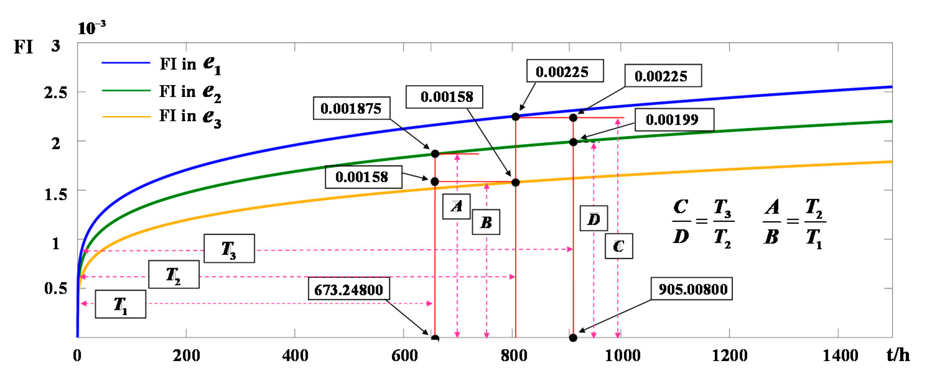
3.2. Improved PIM Which Considers Past Effects

The PIM assumes that the intensity function in different WCs has a proportional relationship. This study seeks to apply the influence of WCs over time through transformations. It is noticed that when the baseline has the form of Weibull process, the transformation can be implemented in PIM. Thus, Equation (13) can be re-expressed as:

$$w(t|e_i)=a_{0}b\cdot {\left({\left(\exp \left({\displaystyle \sum _{l=1}^m{k}_l\cdot \left(Z_l\left(e_i\right)-Z_l\left(e_0\right)\right)}\right)\right)}^{\frac{1}{b}}\cdot t\right)}^{b-1}\cdot {\left(\exp \left({\displaystyle \sum _{l=1}^m{k}_l\cdot \left(Z_l\left(e_i\right)-Z_l\left(e_0\right)\right)}\right)\right)}^{\frac{1}{b}},$$

(15)

In Equation (15), the effects of WCs on the FI are divided into two parts. One of which acts directly on the FI, the other indirectly affects the FI by changing the time scale. When these two parts have the same form, they have the basic characteristics of the AM. Compared with Equation (10), we can regard this segmented effect as the unit time damage in $e_k$, which takes $e_0$ as the standard WC. When the segmented effect is multiplied by time $t$, it can be regarded as the cumulative damage up to $t$, as shown in Equation (16).

$$w(t|e_i)=a_{0}b\cdot {\left(M(0,t|e_i)\right)}^{b-1}\cdot m(0,t|e_i),$$

(16)

Here, the standard WC is simply a reference standard, and there are no specific requirements of the WC itself. Any WC can be set as the standard WC, all other WCs thereafter are based on it as the reference standard. Given that Equation (10) shows that the FI is a function of cumulative damage, assuming that the unit damage under any WC is 1, it will only lead to a change in the function between the cumulative damage and the FI and will not affect the reference of other functions.

Therefore, the dynamic form of WCs needs discussion. Supposing that the system runs in a dynamic WC $E_2$, where the system works in $e_1$ from $t_0(t_0=0)$ to $t_1$, in $e_2$ from $t_1$ to $t_2$. As the unit time damage of the systems is not equal in each WC, the FI function also has unequal characteristics in each WC. When $t_0\le t<t_1$, the cumulative damage of the system can be expressed as $M(0,t|e_1)$. Since it is assumed that the damage per unit time under standard WC is 1, then the cumulative damage can be expressed as:

$$M(0,t)=M(0,t|e_1)={\left(\exp \left({\displaystyle \sum _{l=1}^m{k}_l\cdot \left(Z_l\left(e_1\right)-Z_l\left(e_0\right)\right)}\right)\right)}^{\frac{1}{b}}\cdot t,$$

(17)

The unit time damage is:

$$m(0,t|e_1)={\left(\exp \left({\displaystyle \sum _{l=1}^m{k}_l\cdot \left(Z_l\left(e_1\right)-Z_l\left(e_0\right)\right)}\right)\right)}^{\frac{1}{b}},$$

(18)

Applying Equations (17) and (18) into Equation (16) results in:

$$w(t|e_1)=a_{0}b\cdot {\left(t\right)}^{b-1}\cdot \left(\exp \left({\displaystyle \sum _{l=1}^m{k}_l\cdot \left(Z_l\left(e_1\right)-Z_l\left(e_0\right)\right)}\right)\right),$$

(19)

When $t_1\le t<t_2$, the cumulative damage can be divided into two parts: the first part is the cumulative damage in $e_1$ from $t_0(t_0=0)$ to $t_1$, the second part is the cumulative damage in $e_2$ from $t_1$ to $t_2$. FI function can be derived as:

$$\begin{array}{l}w(t|E_2)=\underset{\Delta t\to 0}{\lim }\frac{W(M(0,t_1|e_1)+M(t_1,t|e_2)+M(t,t+\Delta t|e_2))-W(M(0,t_1|e_1)+M(t_1,t|e_2))}{\Delta t}\\ =\underset{\Delta t\to 0}{\lim }\frac{W(M(0,t_1|e_1)+M(t_1,t|e_2)+M(t,t+\Delta t|e_2))-W(M(0,t_1|e_1)+M(t_1,t|e_2))}{\Delta t\cdot M(t,t+\Delta t|e_2)}\cdot \frac{M(t,t+\Delta t|e_2)}{\Delta t}\\ =m(t|e_2)\cdot w_0(M(0,t_1|e_1)+M(t_1,t|e_2))\end{array},$$

(20)

So, Equation (16) can be rewritten as follows:

$$w(t|e_i)=a_{0}b\cdot {\left(M(0,t_1|e_1)+M(t_1,t|e_2)\right)}^{b-1}\cdot m(0,t|e_2),$$

(21)

The total cumulative damage is the sum of the two parts of damage, which is shown in Equation (22):

$$\begin{array}{l}M(0,t)=M(0,t_1|e_1)+M(t_1,t|e_2)=\\ {\left(\exp \left({\displaystyle \sum _{l=1}^m{k}_l\cdot \left(Z_l\left(e_1\right)-Z_l\left(e_0\right)\right)}\right)\right)}^{\frac{1}{b}}\cdot \left(t_1-t_0\right)+{\left(\exp \left({\displaystyle \sum _{l=1}^m{k}_l\cdot \left(Z_l\left(e_2\right)-Z_l\left(e_0\right)\right)}\right)\right)}^{\frac{1}{b}}\cdot \left(t-t_1\right)\end{array},$$

(22)

The unit time damage currently is:

$$m(0,t|e_2)={\left(\exp \left({\displaystyle \sum _{l=1}^m{k}_l\cdot \left(Z_l\left(e_2\right)-Z_l\left(e_0\right)\right)}\right)\right)}^{\frac{1}{b}},$$

(23)

Applying Equations (22) and (23) into Equation (21) leads to:

$$\begin{array}{l}w(t|E_2)={\left(\exp \left({\displaystyle \sum _{l=1}^m{k}_l\cdot \left(Z_l\left(e_2\right)-Z_l\left(e_0\right)\right)}\right)\right)}^{\frac{1}{b}}\cdot a_{0}b\cdot \\ {\left(\left({\left(\exp \left({\displaystyle \sum _{l=1}^m{k}_l\cdot \left(Z_l\left(e_1\right)-Z_l\left(e_0\right)\right)}\right)\right)}^{\frac{1}{b}}\cdot \left(t_1-t_0\right)+{\left(\exp \left({\displaystyle \sum _{l=1}^m{k}_l\cdot \left(Z_l\left(e_2\right)-Z_l\left(e_0\right)\right)}\right)\right)}^{\frac{1}{b}}\cdot \left(t-t_1\right)\right)\right)}^{b-1}\end{array},$$

(24)

The general case can then be discussed. Supposing the system runs in a dynamic WC $E_n$, where the system works in $e_1$ from $t_0(t_0=0)$ to $t_1$, in $e_2$ from $t_1$ to $t_2$, in $e_n$ from $t_{n-1}$ to $t_n$. When $t_{n-1}\le t\le t_n$, the FI function can be derived as:

$$\begin{array}{l}w(t|E_n)\\ =\underset{\Delta t\to 0}{\lim }\frac{W({\displaystyle \sum _{i=1}^{n-1}M(t_{i-1},t_i|e_i)}+M(t_{n-1},t|e_n)+M(t,t+\Delta t|e_n))-W({\displaystyle \sum _{i=1}^{n-1}M(t_{i-1},t_i|e_i)}+M(t_{n-1},t|e_n))}{\Delta t}\\ =\underset{\Delta t\to 0}{\lim }\frac{W({\displaystyle \sum _{i=1}^{n-1}M(t_{i-1},t_i|e_i)}+M(t_{n-1},t|e_n))-W({\displaystyle \sum _{i=1}^{n-1}M(t_{i-1},t_i|e_i)}+M(t_{n-1},t|e_n))}{\Delta t\cdot M(t,t+\Delta t|e_n)}\cdot \frac{M(t,t+\Delta t|e_n)}{\Delta t}\\ =m(t|e_n)\cdot w_0({\displaystyle \sum _{i=1}^{n-1}M(t_{i-1},t_i|e_i)}+M(t_{n-1},t|e_n))\end{array},$$

(25)

Equation (16) is rewritten as follows:

$$w(t|e_n)=a_{0}b\cdot {\left({\displaystyle \sum _{i=1}^{n-1}M(t_{i-1},t_i|e_i)}+M(t_{n-1},t|e_n)\right)}^{b-1}\cdot m(0,t|e_n),$$

(26)

The total cumulative damage is the sum of all parts of damage, which is shown in Equation (27):

$$\begin{array}{l}M(0,t|E_n)={\displaystyle \sum _{i=1}^{n-1}M(t_{i-1},t_i|e_i)}+M(t_{n-1},t|e_n)\\ ={\displaystyle \sum _{i=1}^{n-1}\left({\left(\exp \left({\displaystyle \sum _{l=1}^m{k}_l\cdot \left(Z_l\left(e_i\right)-Z_l\left(e_0\right)\right)}\right)\right)}^{\frac{1}{\beta }}\cdot \left(t_i-t_{i-1}\right)\right)}+{\left(\exp \left({\displaystyle \sum _{l=1}^m{k}_l\cdot \left(Z_l\left(e_n\right)-Z_l\left(e_0\right)\right)}\right)\right)}^{\frac{1}{\beta }}\cdot \left(t-t_{n-1}\right)\end{array},$$

(27)

The current unit time damage is:

$$m(0,t|e_i)={\left(\exp \left({\displaystyle \sum _{l=1}^m{k}_l\cdot \left(Z_l\left(e_i\right)-Z_l\left(e_0\right)\right)}\right)\right)}^{\frac{1}{\beta }},$$

(28)

Applying Equations (27) and (28) into Equation (26) leads to:

$$\begin{array}{l}w(t|E_n)={\left(\exp \left({\displaystyle \sum _{l=1}^m{k}_l\cdot \left(Z_l\left(e_n\right)-Z_l\left(e_0\right)\right)}\right)\right)}^{\frac{1}{b}}\cdot a_{0}b\cdot \\ {\left(\left({\displaystyle \sum _{i=1}^{n-1}\left({\left(\exp \left({\displaystyle \sum _{l=1}^m{k}_l\cdot \left(Z_l\left(e_i\right)-Z_l\left(e_0\right)\right)}\right)\right)}^{\frac{1}{b}}\cdot \left(t_i-t_{i-1}\right)\right)}+{\left(\exp \left({\displaystyle \sum _{l=1}^m{k}_l\cdot \left(Z_l\left(e_n\right)-Z_l\left(e_0\right)\right)}\right)\right)}^{\frac{1}{b}}\cdot \left(t-t_{n-1}\right)\right)\right)}^{b-1}\end{array},$$

(29)

where the FI in dynamic WCs is expressed by the form of that in standard WCs.

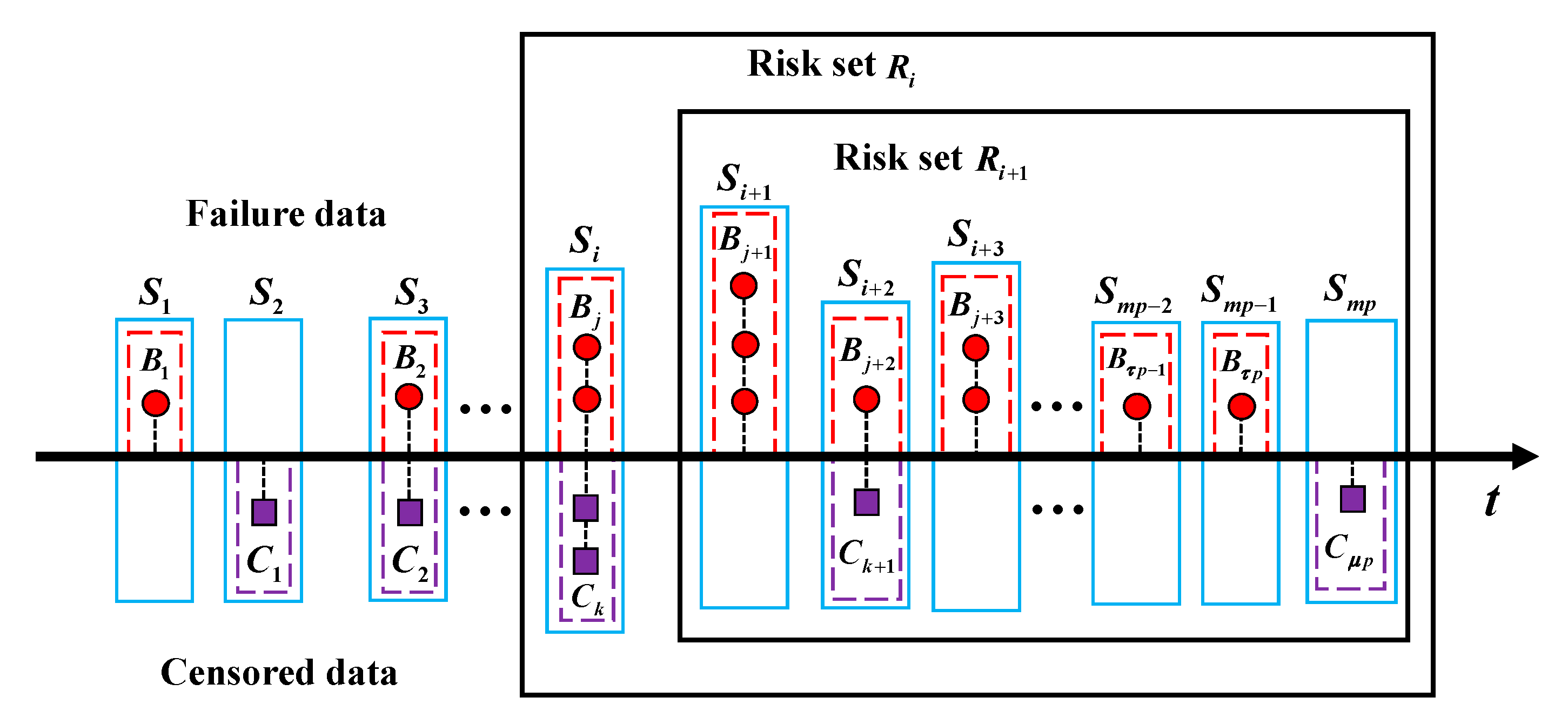
3.3. Model Estimation

The parameter estimation of the PIM with a Weibull process as a baseline intensity can refer to the solutions in the literature [17,33]. Firstly, the covariate coefficients are estimated by using the partial likelihood estimation method [34]. Then the shape and scale parameters in the Weibull function can be estimated according to the maximum likelihood estimation method. In the estimation of covariate coefficients, the WC factors that have little impact on the FI can be eliminated by the likelihood ratio test [35].

The end-of-life data and censored data are distinguished in the partial likelihood estimation. Supposing that there are $np$ units of observation, each unit is composed of an observation time and a covariate group. For example, the i-th individual unit of observation $\left(t_i,Z\left(i\right)\right)$ is composed of the observation time $t_i$ and the covariate vector $Z\left(i\right)$. The $np$ individual units of observation are arranged in descending observation times to obtain the $mp$ of individual unit of observation groups. The i-th unit of observation group is denoted as $S_i$. Since the observation times in different individual units of observation may be equal, there is $mp\le np$. Supposing that among all individual units of observation there are $kp$ individual units of observation whose observation times are end-of-life data, the remaining $np-kp$ individual units’ observation times are censored. Arranging the $kp$ individual units of observation with end-of-life observation times in ascending order obtains $\tau p$ end-of-life groups with different observation times. Then, recording the i-th group as $B_j$, the number individual unit of observation are denoted in $B_j$ as $b_j$. Arranging the remaining $np-kp$ individual units of observation whose observation time belongs to the censored data in ascending order, obtains $\mu p$ censored groups with different observation times. Then, the k-th group is recorded as $C_k$. Since the observation time in different individual units of observation may be equal, there are $\tau p\le kp$, $\mu p\le np-kp$. For the observation time $t$ of a specific individual unit of observation, all units of observation that have not expired and are not censored at that moment constitute the risk group, and the risk set corresponding to the observation time $t_i$ can be denoted as $R_i$. The specific definition results are shown in Figure 2.

Therefore, the partial likelihood estimation function can be expressed as:

$$L(K)={\displaystyle \sum _{j=1}^{\tau p}\frac{{\displaystyle \prod _{i\in B_j}{g}_0\left(Z\left(i\right),K\right)}}{{\left({\displaystyle \sum _{i\in R_j}{g}_0\left(Z\left(i\right),K\right)}\right)}^{b_j}}},$$

(30)

where $K$ is the coefficient vector. In this paper, all the covariate functions are considered as exponential functions. Then the covariate coefficients can be obtained by Equation (31),

$$\frac{\partial \ln L(K)}{\partial k_i}={\displaystyle \sum _{j=1}^{\tau p}({\displaystyle \sum _{i\in B_j}^{}Z\left(i\right)K}-b_j{\displaystyle \sum _{i\in R_j}\frac{Z\left(i\right)\exp (Z\left(i\right)K)}{{\displaystyle \sum _{i\in R_j}\exp (Z\left(i\right)K)}}})},$$

(31)

The criterion for judging the impact of WC factors is to build likelihood ratio statistics as Equation (32).

$$H^2(d)=-2\ln \left(\frac{L\left(K\right)}{L\left(K_i\right)}\right),$$

(32)

where $L\left(K\right)$ is the partial likelihood function which contains the $k_i$, $L\left(K_i\right)$ is the partial likelihood function without $k_i$; compare the $H^2(d)$ with the Chi-square distribution ${\lambda }_{\alpha }{}^2(d)$. After covariate coefficients are all determined according to the above statement, the parameters in the Weibull function can be estimated though the maximum likelihood method.

4. Case Study

4.1. Numerical Cases

In order to show the features and advantages of the proposed method, a numerical case is first used to explain and illustrate it. It is assumed that the failure data of an electromechanical system obey the Weibull distribution. The parameters of the Weibull function are as follows: $a=2.0183\times {10}^{-4}$, $b=1.2$. The factors in the WCs are $Z_1$, $Z_2$, and $Z_3$ and their corresponding coefficients are $k_1=1.1$, $k_2=0.5$, and $k_3=0.04$. $e_1$, $e_2$, and $e_3$ indicate three different WCs in the operation of the system. The specific value of these factors in three WCs are: $Z_1\left(e_1\right)=0.12$, $Z_2\left(e_1\right)=0.8$, $Z_3\left(e_1\right)=9$; $Z_1\left(e_2\right)=0.04$, $Z_2\left(e_2\right)=0.2$, $Z_3\left(e_2\right)=15$; and $Z_1\left(e_3\right)=0.07$, $Z_2\left(e_3\right)=0.6$, $Z_3\left(e_3\right)=4$ respectively. Since there is no special restriction on the selection of standard WCs, we set $e_2$ as the standard WC. The FIs from 0 to 1500 under the three WCs are shown in Figure 3.

Comparing the FIs in $e_1$ and $e_2$, it can be seen that the FI in $e_1$ is always greater than that in $e_2$, which means that the combined effect of each factor in $e_1$ is more likely to cause failure than that in $e_2$. By using Equation (10), it can be discerned that the unit time damage in $e_1$ is 1.13 times the unit time damage in $e_2$. Based on this, the relationship of the cumulative damage between these two WCs throughout the same time span can be obtained. For example, the cumulative damage from 0 to 800 h in $e_1$ is equal to the cumulative damage from 0 to 905.00800 h in $e_2$. Equal cumulative damage does not mean the same FI, which is also related to the current WC. For example, the FI at 800 h is 0.00225 in $e_1$,which is not equal to the FI at 905.00800 h, which is 0.00199. Though their cumulative damage is equal at this point, the ratio of their FIs is also equal to 1.13. Comparing the FIs in $e_2$ and $e_3$, it can be seen that the FI in $e_3$ is always lower than in $e_2$, which means that the combined effect of each factor in $e_3$ is less likely to cause failure than that in $e_2$. The unit time damage in $e_3$ is 0.84 times the unit time damage in $e_2$. So, the cumulative damage from 0 to 800 h in $e_3$ is equal to the cumulative damage from 0 to 673.24800 h in $e_2$. The FI in $e_3$ at 800 h is 0.00158, which is 0.84 times the FI in $e_2$ at 673.24800 h.

The above case shows the differences between static WCs, which always maintain a constant level. Consider the following different situations in dynamic WCs with the basic parameters unchanged. Situation 1: the system operates in $e_1$ from 0 to 1000 h, in $e_3$ from 1000 h to 3000 h, in $e_2$ from 3000 h to 5000 h. Situation 2: the system operates in $e_3$ from 0 to 2000 h, in $e_1$ from 2000 h to 3000 h, in $e_2$ from 3000 h to 5000 h. The results of the two situations are shown in Figure 4.

Figure 4 shows that the values of the FI are mutated at certain points in time due to changes in the WCs. In Situation 1, the WC transforms from $e_1$ to $e_3$ at 1000 h, which causes the change of the FI value from 0.00235 to 0.00175. The translation of WC from $e_3$ to $e_2$ at 3000 h causes the change of the FI value from 0.00210 to 0.00250. Though the system works in $e_3$ from 1000 h to 3000 h, the FI is always larger than that in $e_3$. The reason is that the system operates in $e_1$ from 0 to 1000 h, which generates more damage than working in $e_3$ from 0 to 1000 h. The same explanation can be given when the FI is less than that working in $e_2$ from 3000 h to 5000 h, because the cumulative damage of the system at 3000 h is less than that always working in $e_2$. In Situation 2, the transformation of the WC leads to the change of the FI value from 0.00189 to 0.00255 at 2000 h, and from 0.00282 to 0.00250 at 3000 h. The differences in the cumulative damage resulting in the FI is less than that in $e_1$ from 2000 h to 3000 h, in $e_2$ from 3000 h to 5000 h. The reason that the FI in situations 1 and 2 is the same from 3000 h to 5000 h is that the cumulative damage and WC are all the same from 3000 h to 5000 h.

4.2. Real-World Cases

This section takes motorized spindles, which are used in the machining centers, as an example to confirm the practicability of the method proposed in this paper. According to engineering experience, cutting force, rotational speed, cutting fluid, and number of tool changes are selected as the four WC factors, which may have different influences on FI. They are represented by $Z_1$, $Z_2$, $Z_3$, and $Z_4$ with the corresponding coefficients $k_1$, $k_2$, $k_3$, and $k_4$. There are eight different WCs when the motorized spindles operate. The exact parameters in these WCs are shown in

Table 1. The specific value of parameters in the 8 working conditions.

Working Conditions	${\mathit{Z}}_1\left(\mathbf{KN}\right)$	${\mathit{Z}}_2(\mathbf{r}/\mathbf{min})$	${\mathit{Z}}_3$	${\mathit{Z}}_4$
$e_1$	0.25	2200	1	10
$e_2$	0.23	3500	0	12
$e_3$	0.39	2800	1	6
$e_4$	0.42	1800	1	6
$e_5$	0.26	4200	0	2
$e_6$	0.13	3500	1	9
$e_7$	0.51	3000	1	6
$e_8$	0.60	3600	1	8

. In $Z_3$, 1 means using cutting fluid, 0 means not using cutting fluid.

In the likelihood ratio test, $\alpha$ is set as 0.05. When the numbers of covariates are 4 and 3, the test does not meet the criteria. When the number is 2, and the covariables are rotational speed and number of tool changes, respectively, the test meets the standard. Thus, the two covariates are identified as the factors that influence the FI. The coefficients of these two factors are estimated by the partial likelihood estimation, with the results shown in

Table 2. The results of coefficients of all WC factors.

Covariate Number	Working Conditions Covariates
	${\mathit{k}}_1$	${\mathit{k}}_2$	${\mathit{k}}_3$	${\mathit{k}}_4$	${\mathit{H}}^2$	${\mathit{\lambda }}_{0.05}{}^2$
4	−0.510233	0.000505	0.012975	−0.080421	7.603	9.488
3	−0.493228	0.000500	0	−0.080318	7.602	7.815
2	0	0.000536	0	−0.075618	7.503	5.991

.

By using the maximum likelihood estimation, the shape and scale parameters of the Weibull function are estimated, which are $a=0.0013$ and $b=0.8829$. For further explanation, a set of dynamic WCs can be built to compare the difference between the traditional and the proposed PIMs. First, it is assumed that the motorized spindles operate in $e_5$ from 0 to 500 h, in $e_8$ from 500 h to 1000 h, in $e_6$ from 1000 h to 1500 h, in $e_7$ from 1500 h to 2000 h, in $e_3$ from 2000 h to 2500 h, in $e_2$ from 2500 h to 3000 h, in $e_4$ 3000 h to 3500 h, and in $e_1$ from 3500 to 4000. Then, the FIs calculated by the traditional PIM and the PIM, which consider the past effects, are shown in Figure 5. The exact results at specific points in time are shown in

Table 3. The results at specific points in time.

Working Condition	${\mathit{e}}_5$		${\mathit{e}}_8$		${\mathit{e}}_6$		${\mathit{e}}_7$
Time	0	500	500	1000	1000	1500	1500	2000
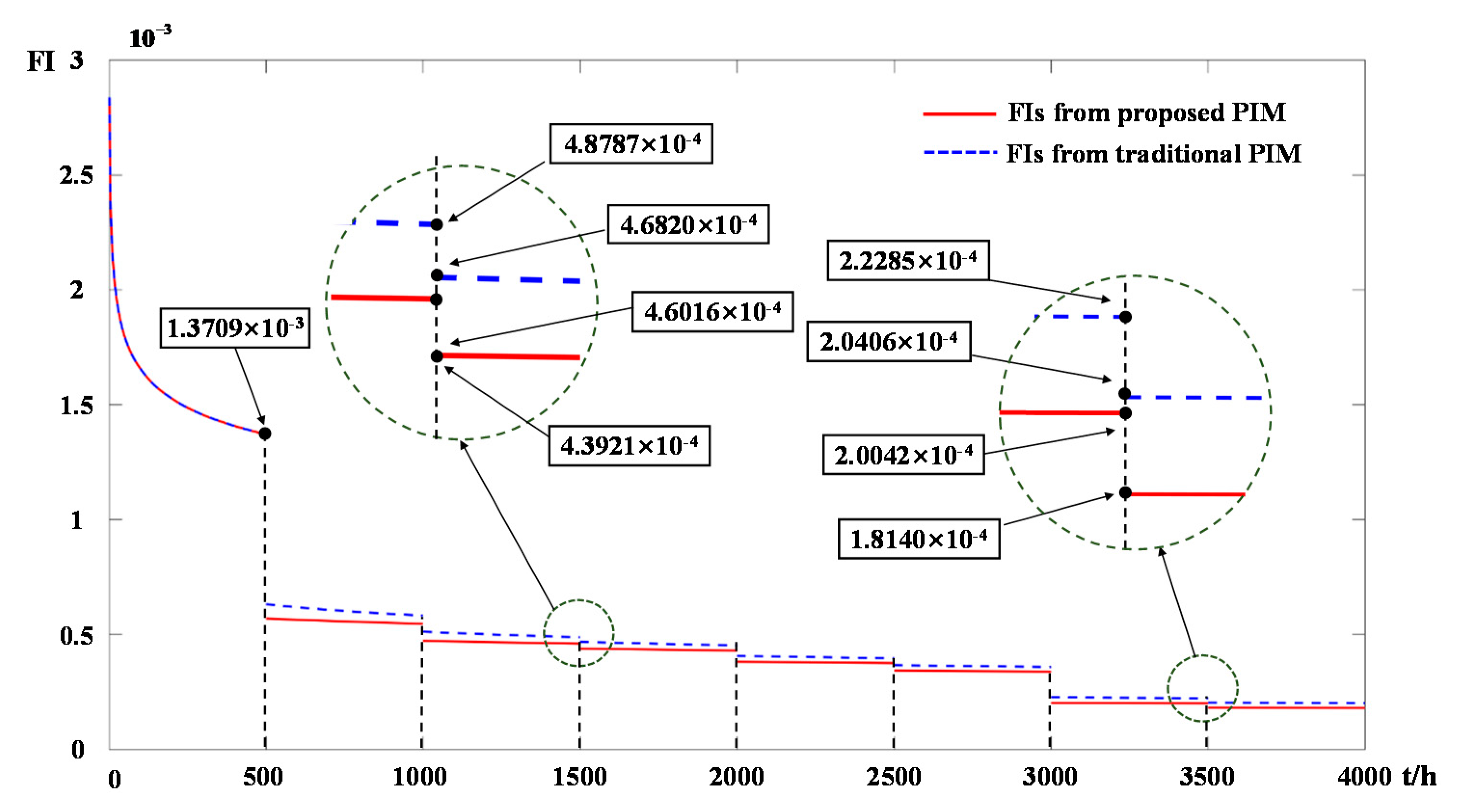
Proposed PIM	0	13.7089 $\times$ 10−4	5.6969 $\times$ 10−4	5.4697 $\times$ 10−4	4.7250 $\times$ 10−4	4.6016 $\times$ 10−4	4.3921 $\times$ 10−4	4.3022 $\times$ 10−4
Traditional PIM	0	13.7089 $\times$ 10−4	6.3138 $\times$ 10−4	5.8216 $\times$ 10−4	5.1159 $\times$ 10−4	4.8787 $\times$ 10−4	4.6820 $\times$ 10−4	4.5270 $\times$ 10−4
Working Condition	${\mathit{e}}_3$		${\mathit{e}}_2$		${\mathit{e}}_4$		${\mathit{e}}_1$
Time	2000	2500	2500	3000	3000	3500	3500	4000
Proposed PIM	3.8103 $\times$ 10−4	3.7510 $\times$ 10−4	3.4319 $\times$ 10−4	3.3885 $\times$ 10−4	2.0183 $\times$ 10−4	2.0042 $\times$ 10−4	1.8140 $\times$ 10−4	1.8032 $\times$ 10−4
Traditional PIM	4.0668 $\times$ 10−4	3.9619 $\times$ 10−4	3.6628 $\times$ 10−4	3.5854 $\times$ 10−4	2.2691 $\times$ 10−4	2.2285 $\times$ 10−4	2.0406 $\times$ 10−4	2.0090 $\times$ 10−4

.

In this case, with $b=0.8829<1$, the system can be seen as gradually improving. The FI decreases with the increase of service time. This situation usually occurs in the early failure period of electromechanical systems. In other words, at this stage the FI decreases with the increase of cumulative damage. As shown in Figure 5 and Table 3, the results calculated by the proposed PIM are always smaller than those of the traditional PIM, except from 0 to 500 h. The reason for this is that the proposed method considers the influence of past effects. In these built dynamic WCs, which are arranged in descending order of severity, the cumulative damage at a specific moment is always greater than the cumulative damage assumed to always exist in the current state. In the 0 to 500 h period, since no other specific WCs appeared beforehand, the calculation results of the two methods are the same. On the other hand, FIs can change abruptly with sudden changes in WCs, because the FI is not only related to cumulative damage, but also to the current WCs. Through the proposed PIM, we explored the influences of WCs on FIs of repairable systems, which makes up for the flaws in the traditional method. Due to the limitation of the model’s characteristics, taking the WC factor as an independent individual, the more complex couplings among them may be ignored, which could regretfully cause inaccurate calculations. On the other hand, for multipart systems, with the extension of device service time, the correlation between components gradually highlights the effects on the FI, which is also one of the points we need to pay attention to in the future.

5. Conclusions

This paper proposes an improved PIM that considers the past effects of WCs. Drawbacks of traditional PIM which cannot be applied to the dynamic WCs are eliminated by this method. It is suitable for the electromechanical systems with a Weibull process as a baseline intensity. The contacts over time, working conditions, and failure probability are first explained from the perspective of damage, which converts the original probability function with time to the composite function related to time. The operation time is regarded as cumulative damage under different WCs. Through the equivalent damage model, which is the interpretation of the equivalent time model from the perspective of damage, the cumulative damage in different WCs is converted to standard WCs. By using the advantages of parameter estimation in the PIM, the influence of WCs on the FI is estimated. Then, the linear assumption is introduced in the PIM when its baseline function can be seen as a Weibull process, especially for electromechanical systems. Thus, the FIs in dynamic WCs can be obtained by the improved method. As can be seen from the results of the case studies, the FIs of electromechanical systems can change suddenly through varying WCs. The cumulative damage and the current WCs are the two main factors affecting the FI.

References

- Wu, T.; Yang, L.; Ma, X.; Zhang, Z.; Zhao, Y. Dynamic maintenance strategy with iteratively updated group information. Reliab. Eng. Syst. Saf. 2020, 197, 106820. [Google Scholar] [CrossRef]
- Fan, D.; Zhang, A.; Feng, Q.; Cai, B.; Liu, Y.; Ren, Y. Group maintenance optimization of subsea Xmas trees with stochastic dependency. Reliab. Eng. Syst. Saf. 2021, 209, 107450. [Google Scholar] [CrossRef]
- Dao, C.; Zuo, M. Optimal selective maintenance for multi-state systems in variable loading conditions. Reliab. Eng. Syst. Saf. 2017, 166, 171–180. [Google Scholar] [CrossRef]
- Li, H.; Deng, Z.M.; Golilarz, N.A.; Soares, C.G. Reliability analysis of the main drive system of a CNC machine tool including early failures. Reliab. Eng. Syst. Saf. 2021, 215, 107846. [Google Scholar] [CrossRef]
- Li, H.; Soares, C.G.; Huang, H.Z. Reliability analysis of a floating offshore wind turbine using Bayesian Networks. Ocean Eng. 2020, 217, 107827. [Google Scholar] [CrossRef]
- Jia, X.; Cui, L.; Xing, L. New insights into reliability problems for supply chains management based on conventional reliability model. Eksploat. I Niezawodn. 2018, 20, 465–470. [Google Scholar] [CrossRef]
- Niu, X.; Wang, R.; Liao, D.; Zhu, S.; Zhang, X.; Keshtegar, B. Probabilistic modeling of uncertainties in fatigue reliability analysis of turbine bladed disks. Int. J. Fatigue 2021, 142, 105912. [Google Scholar] [CrossRef]
- Hu, W.; Westerlund, P.; Hilber, P.; Chen, C.; Yang, Z. A general model, estimation, and procedure for modeling recurrent failure process of high-voltage circuit breakers considering multivariate impacts. Reliab. Eng. Syst. Saf. 2022, 220, 108276. [Google Scholar] [CrossRef]
- Cheng, Q.; Qi, B.; Liu, Z.; Zhang, C.; Xue, D. An accuracy degradation analysis of ball screw mechanism considering time-varying motion and loading working conditions. Mech. Mach. Theory 2019, 134, 1–23. [Google Scholar] [CrossRef]
- Jia, X.; Xing, L.; Song, X. Aggregated Markov-based reliability analysis of multi-state systems under combined dynamic environments. Qual. Reliab. Eng. Int. 2020, 36, 846–860. [Google Scholar] [CrossRef]
- Cai, Y.; Zhao, Y.; Ma, X.; Zhou, K. Reliability assessment in dynamic field environment incorporating multiple environmental effects. Proc. Inst. Mech. Eng. Part O J. Risk. Reliab. 2020, 234, 3–14. [Google Scholar] [CrossRef]
- Dong, Q.; Cui, L. Reliability analysis of a system with two-stage degradation using Wiener processes with piecewise linear drift. IMA J. Manag. Math. 2021, 32, 3–29. [Google Scholar] [CrossRef]
- Hong, L.; Zhai, Q.; Wang, X.; Ye, Z. System reliability evaluation under dynamic operating conditions. IEEE Trans. Reliab. 2018, 68, 800–809. [Google Scholar] [CrossRef]
- Wang, Y.; Zhou, B.; Ge, T.; Feng, H.; Tao, W. Small-Sample accelerated life test method based on the inverse power law model. Appl. Math. Inform. Sci. 2014, 8, 1725. [Google Scholar] [CrossRef] [Green Version]
- Escobar, L.; Meeker, W. A review of accelerated test models. Stat. Sci. 2006, 21, 552–577. [Google Scholar] [CrossRef] [Green Version]
- Yang, Z.; Li, X.; Chen, C.; Zhao, H.; Yang, D.; Guo, J.; Luo, W. Reliability assessment of the spindle systems with a competing risk model. Proc. Inst. Mech. Eng. Part O J. Risk. Reliab. 2019, 233, 226–234. [Google Scholar] [CrossRef]
- Li, H.; Yang, Z.; Xu, B.; Chen, C.; Kan, Y.; Liu, G. Reliability evaluation of NC machine tools considering working conditions. Math. Probl. Eng. 2016, 206, 9842607. [Google Scholar] [CrossRef] [Green Version]
- Pike, M. A method of analysis of a certain class of experiments in carcinogenesis. Biometrics 1966, 22, 142–161. [Google Scholar] [CrossRef]
- Cox, D.R. Regression models and Life-Tables. J. R. Stat. Soc. Ser. B Stat. Methodol. 1972, 34, 187–202. [Google Scholar] [CrossRef]
- Bokoro, P.; Doorsamy, W. Reliability analysis of low-voltage metal-oxide surge arresters using accelerated failure time model. IEEE Trans. Power Syst. 2018, 33, 3139–3146. [Google Scholar] [CrossRef]
- Bagdonavičius, V.; Levulienė, R. On accelerated life testing when the AFT model fails. IEEE Trans. Reliab. 2019, 68, 1311–1319. [Google Scholar] [CrossRef]
- Su, S. Flexible parametric accelerated failure time model. J. Biopharm. Stat. 2021, 31, 650–667. [Google Scholar] [CrossRef] [PubMed]
- Zhang, J.; He, W.; Li, H. A semiparametric approach for accelerated failure time models with covariates subject to measurement error. Commun. Stat. Simul. Comput. 2014, 43, 329–341. [Google Scholar] [CrossRef]
- Zhu, W.; Fouladirad, M.; Bérenguer, C. Condition-based maintenance policies for a combined wear and shock deterioration model with covariates. Comput. Ind. Eng. 2015, 85, 268–283. [Google Scholar] [CrossRef]
- Wang, Y.; Li, Z.; Shahidehpour, M.; Wu, L.; Guo, C.; Zhu, B. Stochastic co-optimization of midterm and short-term maintenance outage scheduling considering covariates in power systems. IEEE Trans. Power Syst. 2016, 31, 4795–4805. [Google Scholar] [CrossRef]
- Yuan, F.; Kumar, U. Kernelized proportional intensity model for repairable systems considering piecewise operating conditions. IEEE Trans. Reliab. 2012, 61, 618–624. [Google Scholar] [CrossRef]
- Hu, W.; Yang, Z.; Chen, C.; Wu, Y.; Xie, Q. A Weibull-based recurrent regression model for repairable systems considering double effects of operation and maintenance: A case study of machine tools. Eng. Syst. Saf. 2021, 213, 107669. [Google Scholar] [CrossRef]
- Lu, X.; Lin, M. Hazard rate function in dynamic environment. Reliab. Eng. Syst. Saf. 2014, 130, 50–60. [Google Scholar] [CrossRef]
- Hu, J.; Jiang, Z.; Liao, H. Preventive maintenance of a batch production system under time-varying operational condition. Int. J. Prod. Res. 2017, 55, 5681–5705. [Google Scholar] [CrossRef]
- Pang, M.; Platt, R.; Schuster, T.; Abrahamowicz, M. Flexible extension of the accelerated failure time model to account for nonlinear and time-dependent effects of covariates on the hazard. Stat. Methods Med. Res. 2021, 30, 2526–2542. [Google Scholar] [CrossRef]
- Solomon, P. Effect of misspecification of regression model in the analysis of survival data. Biometrika 1984, 71, 291–298. [Google Scholar] [CrossRef]
- Syamsundar, A.; Naikan, V. Imperfect repair proportional intensity models for maintained systems. IEEE Trans. Reliab. 2011, 60, 782–787. [Google Scholar] [CrossRef]
- Xu, B. Study on Reliability Modeling and Analysis of CNC Machine Tools Based on Maintenance Degree. Ph.D. Thesis, Jilin University, Changchun, China, 2011. [Google Scholar]
- Cox, D. Partial likelihood. Biometrika 1975, 62, 269–276. [Google Scholar] [CrossRef]
- Wen, F. Numerical study of likelihood-ratio-test-based single change point estimation. Electron. Lett. 2012, 48, 1532–1533. [Google Scholar] [CrossRef]