Abstract
This paper investigates an ordered partial matching alignment problem, in which the goal is to align two sequences in the presence of potentially non-matching regions. We propose a novel parameter-free dynamic programming alignment method called hidden state time warping that allows an alignment path to switch between two different planes: a “visible” plane corresponding to matching sections and a “hidden” plane corresponding to non-matching sections. By defining two distinct planes, we can allow different types of time warping in each plane (e.g., imposing a maximum warping factor in matching regions while allowing completely unconstrained movements in non-matching regions). The resulting algorithm can determine the optimal continuous alignment path via dynamic programming, and the visible plane induces a (possibly) discontinuous alignment path containing matching regions. We show that this approach outperforms existing parameter-free methods on two different partial matching alignment problems involving speech and music.
1. Introduction
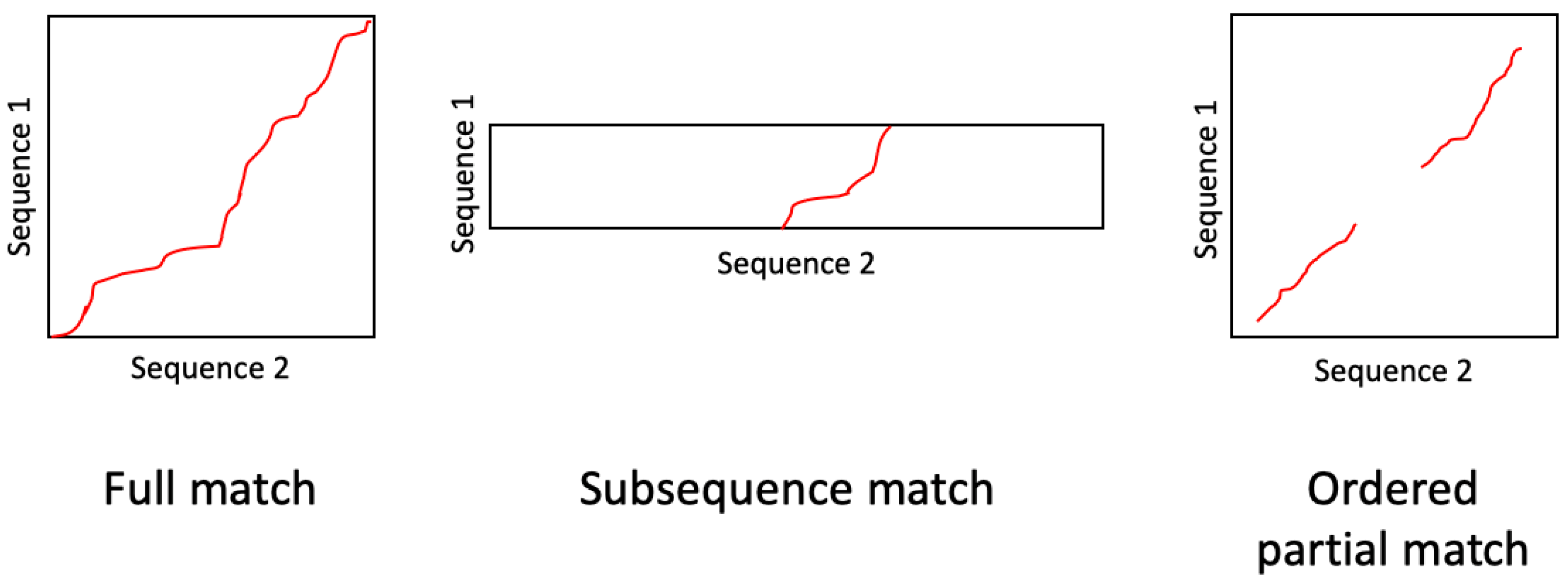
Dynamic time warping (DTW) is a widely used algorithm for determining the optimal alignment between two sequences. Standard DTW assumes that the two sequences start and end at the same location, and that the time warping is defined by a predetermined set of allowable transitions. Variations of DTW have been proposed to estimate alignments under various assumptions and conditions. For example, subsequence DTW determines the optimal alignment between a short query sequence and any subsequence within a longer reference sequence. In this paper, we propose a time warping algorithm for handling ordered partial alignments, where the true alignment between two sequences may contain discontinuities due to non-matching regions but the matching regions are assumed to be ordered. Figure 1 provides a graphical illustration of the difference between the full matching, subsequence matching, and ordered partial matching scenarios.
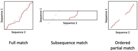
Figure 1.
Different types of alignment problems. HSTW provides a parameter-free solution to the ordered partial match alignment problem.
For the sake of completeness, we provide an overview of standard DTW before describing variations and extensions of it in the literature. Estimating the alignment between two sequences and with DTW consists of three main steps. The first step is to compute a pairwise cost matrix , where indicates the dissimilarity between and . The second step is to compute a cumulative cost matrix , where indicates the lowest cost cumulative path score starting at and ending at . The elements in D can be computed using dynamic programming based on a set of allowable transitions in the cost matrix, and a separate backtrace matrix keeps track of the last transition in the lowest cost path ending at each location. The third step is to follow the backtrace pointers in B to determine the lowest cost path from to .
Many works have proposed variations or extensions of DTW. These works generally fall into one of two categories. The first category focuses on mitigating the quadratic runtime or memory costs of DTW, which make it prohibitive for processing long sequences. Some works approach this by proposing approximations of DTW, e.g., by imposing fixed boundaries on the alignment path (e.g., Sakoe-Chiba band [1] and the Itakura parallelogram [2]), estimating the alignment at a coarse resolution and iteratively refining the alignment path [3,4], estimating the alignment path with a limited amount of memory [5], or using a parallelizable time warping algorithm [6]. Other works approach this by computing exact DTW in a more efficient way, e.g., by using lower bounds [7,8], early abandoning [9,10], utilizing multiple cores [11,12] or specialized hardware [13,14], or performing the dynamic programming along diagonals rather than rows/columns to allow for parallelization [15]. The second category focuses on extending the behavior of DTW in some way. Some examples in the audio processing literature include performing time warping in an online fashion [16,17], handling repeats and jumps in music [18,19,20], handling subsequence alignments [21,22], handling pitch drift in a capella performances [23], and utilizing multiple performances to improve alignment accuracy [24].
This paper proposes an alignment algorithm called hidden state time warping (HSTW) that can handle ordered partial matching. In particular, HSTW allows for aligning two sequences whose alignment may contain discontinuities due to non-matching regions, as shown in Figure 1. Rather than computing a cumulative cost matrix , we instead compute a cumulative cost tensor containing two different planes: a “visible” plane corresponding to matching sections and a “hidden” plane corresponding to non-matching sections. The alignment path can transition between the visible and hidden planes. By defining two distinct planes, we can use different dynamic programming rules to treat matching and non-matching sections differently (e.g., imposing a maximum time warping factor in matching sections while allowing unconstrained movements in non-matching sections). Furthermore, we can find the optimal (continuous) alignment path through the entire double plane using a dynamic programming framework and then induce a discontinuous optimal matching alignment path by considering only the path elements in the visible plane. In the following sections, we describe this algorithm in more detail and provide experimental evidence of its effectiveness on two different tasks: one involving the alignment of speech data in the presence of tampering operations such as insertion, deletion, and replacement, and another involving the synchronization of music performances with different content (e.g., silence or applause) before, after, and in between movements of a musical piece. Code for reproducing our results can be found at https://github.com/HMC-MIR/HSTW (accessed on 5 April 2022).
2. Materials and Methods
In this section, we describe how two partially matching audio recordings can be aligned using our proposed hidden state time warping (HSTW) algorithm. There are three steps: extracting the features, estimating a global alignment, and determining which regions are matching. These three steps will be discussed in the next three subsections (Section 2.1, Section 2.2 and Section 2.3), followed by a discussion of initialization (Section 2.4) and setting hyperparameters (Section 2.5).
2.1. Feature Extraction
The first step is to extract features from both audio recordings. HSTW can work with any feature representation, so for simplicity we use standard feature representations. For speech audio, we compute 13-dimensional MFCCs with delta and delta–delta features (total 39 dimensions) using 25 ms analysis frames and a 10 ms hop size. For music audio, we compute 12-dimensional chroma features based on a constant Q transform with a 23 ms hop size. At the end of this first step, we have two sequences of features and .
2.2. Alignment
The second step is to estimate a global continuous alignment path between the two sequences of features. This process consists of three sub-steps, which are described in the next three paragraphs.
First, we compute a pairwise cost matrix between the two feature sequences. For speech audio, we use Euclidean distance as a dissimilarity metric, and we use cosine distance for music audio. Therefore, indicates the dissimilarity between the feature in the first sequence and the feature in the second sequence.
Second, we compute a cumulative cost tensor (and corresponding backtrace tensor ) using the following dynamic programming rules:
where and correspond to the hidden and visible planes, respectively. In the multi-case expressions for both and , the first case handles the initialization of the cumulative cost tensor, and the second case specifies the dynamic programming rules. There are three types of transitions that end in the hidden plane: (i) a horizontal transition to the right in the hidden plane with a penalty of , (ii) a vertical transition upwards in the hidden plane with a penalty of , and (iii) a diagonal transition from position in the visible plane to position in the hidden plane with penalty . Note that these three cases all incur fixed penalties that are independent of the pairwise cost . There are four types of transitions that end in the visible plane: three regular transitions in the visible plane with corresponding transition weights , as well as a transition from position in the hidden plane to position in the visible plane with a penalty of . As we compute each element of and , we also update the corresponding backtrace tensor entries and to record the optimal transition type at each position.
Third, we determine the optimal global continuous alignment path through D using backtracking. We start with the element in the last row and column of or (whichever has a lower cumulative path score) and then follow the back pointers in B to determine each step of the optimal path. We stop backtracking once we have reached either or .
2.3. Classification
The third step is to classify each element in the optimal global continuous alignment path as matching or not matching. The classification for a path element can then be imputed to the corresponding audio frames in the two recordings. For example, if a path element is classified as a non-match, we can infer that the frame of the first recording does not match the other recording. With the HSTW algorithm, the classification can be done in two ways: (1) classify path elements in the visible plane as matches and path elements in the hidden plane non-matches or (2) classify each path element by applying a hard threshold to the corresponding pairwise cost . We report results with both classification methods.
2.4. Initialization
The equations shown above are not the HSTW algorithm—they are just one example of HSTW. In the same way that DTW can be modified by choosing a different set of allowable transitions and weights or modified to handle subsequence matches, so too can HSTW be flexibly adapted to a range of scenarios.
One way to modify HSTW behavior is to choose different initialization conditions for the cumulative cost tensor D. For example, the equations can be modified to handle subsequence alignment by introducing two changes: (a) initializing , so that the alignment path can begin anywhere in the second (longer) sequence without penalty and (b) beginning the backtracking from position , where to allow the alignment path to end anywhere without penalty. One can treat similarly to allow subsequence paths to start or end in the hidden plane.
Another way to modify HSTW behavior is to choose different allowable transitions and transition weights. The equations shown above allow for , , and transitions within the visible plane with corresponding transition weights 2, 3, and 3. These allowable transitions and transition weights could be chosen differently to encourage or allow certain types of alignment paths.
2.5. Hyperparameters
In addition to the hyperparameters that DTW has, HSTW has three additional hyperparameters: , , and . These three hyperparameters have clear interpretations: is a skip penalty for a horizontal transition, is a skip penalty for a vertical transition, and is a plane transition penalty. These hyperparameters can be set to achieve different types of behavior. We describe our method of setting these hyperparameters for our two tasks of interest.
We set the hyperparameters on our (subsequence alignment) speech verification task to perform well in the presence of common tampering operations such as insertions, deletions, and replacements. For the deletion penalty , we found that the optimal setting is a small, positive number. We want the cost to be small in order to allow skipping in the reference dimension when there is a deletion edit in the query. If we set to zero, however, it allows for arbitrarily long skips, which has undesirable behavior. We use in all of our reported results, and we find that system performance is relatively insensitive to values within the range . For the insertion penalty , we found that the optimal value strongly depends on the values in the cost matrix. If is too large, the algorithm cannot follow vertical alignment paths corresponding to insertions. If is too small, the optimal subsequence path consists of simply skipping across the entire cost matrix. Ideally, we want the penalty to be greater than the cost between two matching elements but smaller than the cost between non-matching elements. Accordingly, we set in a data-dependent way: we calculate the minimum cost in each row of the cost matrix C (i.e., the minimum cost for each query frame), and then set to times the median of these row minima. We find system performance to be insensitive to values across the range . For the hidden-to-visible transition penalty , we find that with works well, and that system performance is insensitive to values within the range . This penalty prevents the alignment path from coming up to the visible plane unless it can “consume” enough low-cost elements.
We set the hyperparameters on our music alignment task in the same manner but with one difference: we always set since the alignment task is symmetric. Based on our training data, we used and .
3. Results
In this section, we describe a set of experiments with two different tasks involving both music and speech data. We first describe the experimental setup of both tasks and then present our empirical results.
3.1. Experimental Setup—Music Synchronization
The first task was the synchronization of different music performances of the same piece in the presence of non-matching regions. We used the Mazurka dataset [25], which consists of multiple performances of five different Chopin Mazurkas. For each performance, the dataset contains manual annotations of beat-level timestamps. We set aside two Mazurkas for training and the other three Mazurkas for testing, resulting in a total of 2514 training alignment pairs and 7069 test alignment pairs. This dataset has been used in a number of previous studies on music alignment [6,25,26,27]. Table 1 shows an overview of the Mazurka dataset.

Table 1.
Overview of the Chopin Mazurka data used in the music alignment task. All durations are in seconds. The top two pieces were used for validation (i.e., setting hyperparameters), and the bottom three pieces were used for testing. Tampered versions of the performances were generated to simulate non-matching regions at the beginning, middle, and end of the recording.
There are a number of factors that might cause two classical music recordings of the same piece to have non-matching regions. For example, a CD audio recording might start and end at the beginning and end of the actual performance, while a Youtube recording might contain silence or applause at the beginning and/or end of the video. Non-matching regions in the middle of a recording might be due to structural differences such as repeats, silence between movements of a piece, and a different cadenza.
We generated tampered versions of the Mazurka performances in order to study the effect of non-matching regions. The beginning, middle, and end of each original Mazurka performance was altered in the following manner. First, a filler audio recording of a different Mazurka was randomly selected from the same train–test split. This filler recording was used to replace original content with non-matching content. Second, the first seconds of the original recording was replaced with a random interval selected from the filler recording, where was selected uniformly in an interval of seconds. Third, the last seconds of the original recording was likewise replaced with a random interval in the filler recording, where was selected uniformly from seconds. Finally, a random L second interval in the middle of the original recording was replaced with content from the filler recording. We ensured that the tampered middle region was at least 10 s away from the tampered regions at the beginning and end, so as to avoid creating very short matching fragments. Each tampered recording was aligned against all other (untampered) original recordings of the same Mazurka.
We evaluated system performance based on how well it classified each audio frame in the query (i.e., the tampered recording) as matching or non-matching. Note that determining whether or not an audio frame was matching or non-matching requires solving the alignment problem accurately. (We found that all systems had roughly the same alignment accuracy, so we only focus on reporting classification performance.) We characterized performance using a standard receiver operating characteristic (ROC) curve, which shows the tradeoff between false positives and false negatives. When evaluating classification performance, we excluded frames that lie within a ms scoring collar around tampering locations.
3.2. Experimental Setup—Speech Alignment & Verification
The second task was to verify the legitimacy of a short speech recording (e.g., a viral video clip of a presidential speech on social media) by comparing it to a trusted reference recording (e.g., an official recording of the entire speech from a major news outlet). The goal was to be able to perform verification in the presence of common tampering operations such as insertions, deletions, and replacements. Note that, while there is a rich literature in audio tampering detection by detecting internal inconsistencies and tampering artifacts (see [28] for a survey), our task instead focuses exclusively on positively verifying the legitimacy of an audio recording by aligning and comparing it to a trusted external reference recording. This problem has become particularly relevant in recent years, as digital audio editing software and deep fake technology has become readily accessible [29].
To simulate a realistic scenario involving a high-profile political figure, we used recordings of former U.S. President Donald Trump. We collected 50 speech recordings of Trump from 2017 to 2018, all taken from the official White House Youtube playlist when he was in office. Each of these recordings is single-speaker and is 1–3 minutes long.
We generated audio queries from the raw data in the following manner. We randomly selected ten 10-second segments from each recording and then generated four different versions of each segment by applying various tampering operations. The first version has no tampering: it is simply an unedited version at a lower bitrate quality (160 kbps) than the reference (320 kbps). The second version has an insertion: we randomly selected an L second fragment from a different audio recording (within the dataset) and inserted the fragment into the 10-second segment at a random location. The third version has a deletion: we randomly selected an L second interval from the segment and deleted it. The fourth version has a replacement: we randomly selected an L second fragment from a different audio recording and used it to replace a randomly selected L second fragment in the 10-second segment. For a given value of L, this process will generate a total of queries. We divided the queries by speech recording and used 50% for training and 50% for testing. Each query was aligned against the corresponding high-resolution reference audio recording from which it was taken.
We evaluated our speech verification system based on how well it classified each audio frame in the query as matching or non-matching. Again, we note that solving the classification task requires solving the alignment task accurately, and is therefore a more reliable indicator of system-level performance. We evaluated this binary classification task using a standard ROC curve and corresponding equal error rate (EER). We excluded frames that lie within a ms scoring collar around tampering locations.
3.3. Speech Alignment & Verification Results
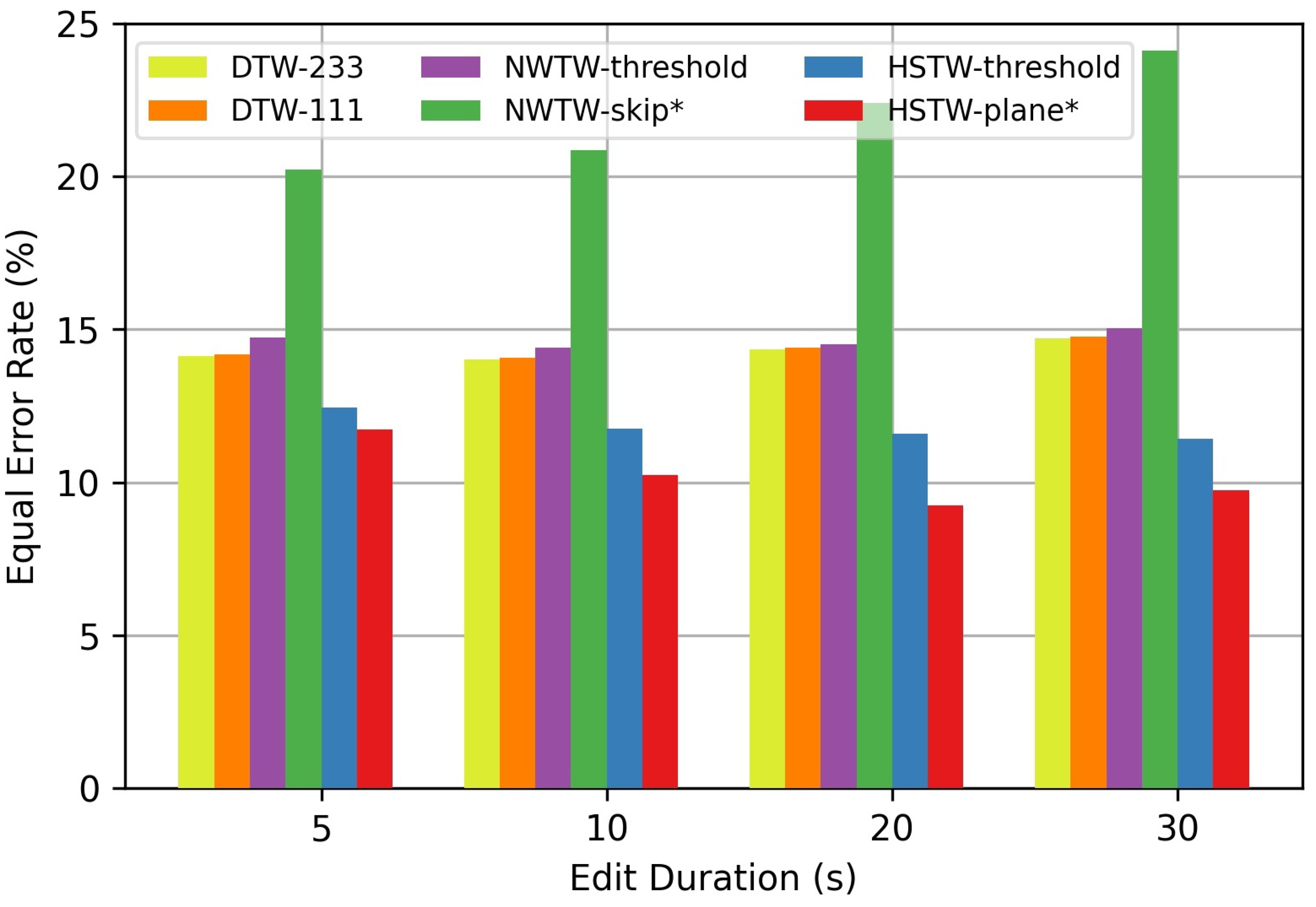
For the speech task, we compared the performance of seven different parameter-free alignment systems. The first system (“DTW-111”) was subsequence DTW with (query, reference) transitions and corresponding transition weights . For each element on the optimal alignment path, the pairwise cost was imputed as a score to the frame in the query (i.e., the potentially tampered recording), and each query frame’s score was compared to a threshold to determine if the frame was a match or a non-match. This threshold can be varied to sweep out an ROC curve. The second (“DTW-121”) and third (“DTW-112”) systems were the same as the first system but with transition weights and , respectively. The fourth system (“NW-threshold”) was Needleman–Wunsch alignment [30], which allows for regular transitions as well as and transitions with a fixed insertion/deletion penalty that does not depend on the pairwise cost matrix C. Once the optimal alignment path was estimated, scores were imputed to the query frames and thresholded, as before. The fifth system (“NW-skip”) was identical to the fourth system but simply classified insertions and deletions as non-matches and transitions as matches. The sixth system (“HSTW-threshold”) used our proposed algorithm to estimate an optimal subsequence alignment path, imputed scores to each query frame based on the pairwise cost matrix, and then applied a threshold. The seventh system (“HSTW-plane”) estimated the alignment with our proposed algorithm and simply classified path elements in the visible plane as matches and path elements in the hidden plane as non-matches. For each system above, hyperparameters were tuned on the training set.
Figure 2 shows the frame classification results on the speech verification task for s tampering durations. For all threshold-based systems (i.e., all systems except NW-skip and HSTW-plane), the bars indicate the EER of classification performance. Because NW-skip and HSTW-plane are not threshold-based systems, their performance is defined by a single point in the ROC plane, as shown in Figure 3 for s tampering durations. For these two systems, an approximation of EER was estimated by averaging the false positive and false negative rate.
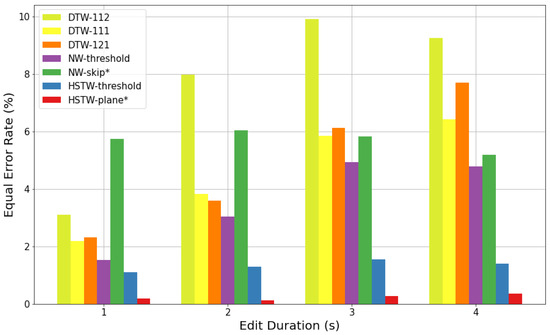
Figure 2.
Results on the speech alignment & verification task. Bars indicate the equal error rate for classifying audio frames as matching vs. non-matching. Systems with are not threshold-based and therefore do not sweep out a full ROC curve. For these systems, the bar indicates the mean values of the false positive and false negative rates.
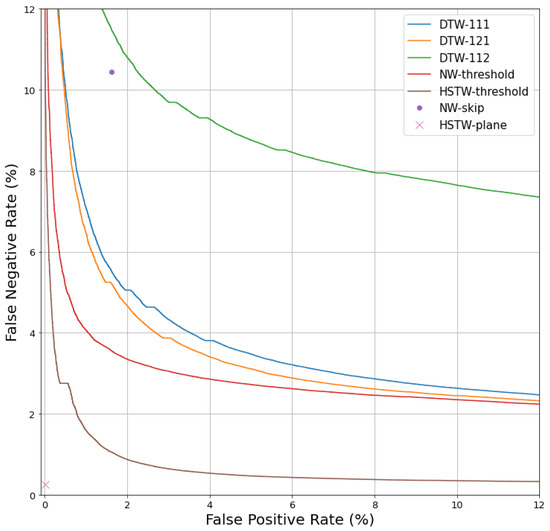
Figure 3.
ROC curves for all systems on the speech alignment & verification task with a s tampering duration. NW-skip and HSTW-plane are not threshold-based systems, so their performance is characterized by a single point.
There are three phenomena to notice in Figure 2 and Figure 3. First, HSTW-plane shows the best classification performance by a wide margin. For example, for s tampering operations, HSTW-plane achieved a false positive rate and a false negative rate, while the best non-HSTW system achieved a equal error rate. Second, HSTW-plane greatly outperformed HSTW-threshold, even though both systems have identical alignment paths. This indicates that there is relevant information in the visible/hidden dimension that is not captured by the 2D alignment between the two sequences. Third, the performance of non-HSTW systems varied drastically based on the tampering duration, but that of the HSTW-based systems was much more stable.
3.4. Music Synchronization Results
For the music task, we compared the performance of six different systems. The first two systems (“DTW-233” and “DTW-111”) were standard DTW with transitions and corresponding transition weights or . Scores were imputed to each frame in the query (i.e., the tampered recording) and thresholded, as before. The third system (“NWTW-threshold”) was proposed in [20] as a way to handle time warping as well as insertions and deletions. It allowed for transitions to handle time warping, as well as and skip transitions with a fixed penalty . Scores were imputed to the query frames and thresholded, as above. The fourth system (“NWTW-skip”) was identical to the third system but simply classified insertion and deletion transitions as non-matches and all other regular transitions as matches. The fifth system (“HSTW-threshold”) used our proposed algorithm to estimate an optimal global alignment path and then imputed scores to each query frame and thresholds, as before. The sixth system (“HSTW-plane”) estimated the alignment with our proposed algorithm and simply classified path elements in the visible plane as matches and path elements in the hidden plane as non-matches. For each system above, hyperparameters were tuned on the training set.
Figure 4 shows the results on the music synchronization task with s tampering durations. We can see that HSTW-plane again had the best performance, but that the music task was much more challenging than the speech task based on the equal error rates. This is because the speech task involves comparing two exactly matching recordings (with possible tampering operations), whereas the music task involves comparing two different performances of a piece (with additional tampering operations). Again, we can see that HSTW-plane outperformed HSTW-threshold despite the fact that both shared the same predicted alignment path. This suggests that the hidden and visible planes are capturing important and relevant information that the 2D alignment path is not capturing.
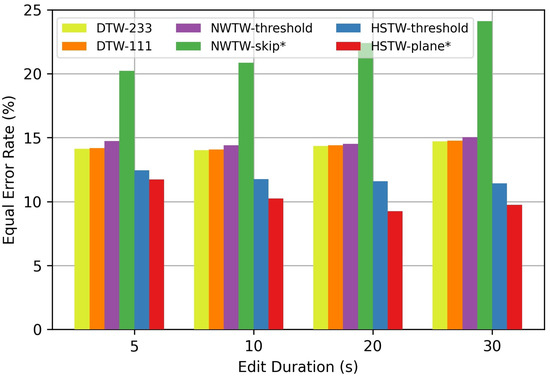
Figure 4.
Results on the music synchronization task with non-matching regions. Bars indicate the equal error rate for classifying audio frames as matching vs. non-matching. For systems that are not threshold-based (indicated with ), bars indicate the mean values of the false positive and false negative rates.
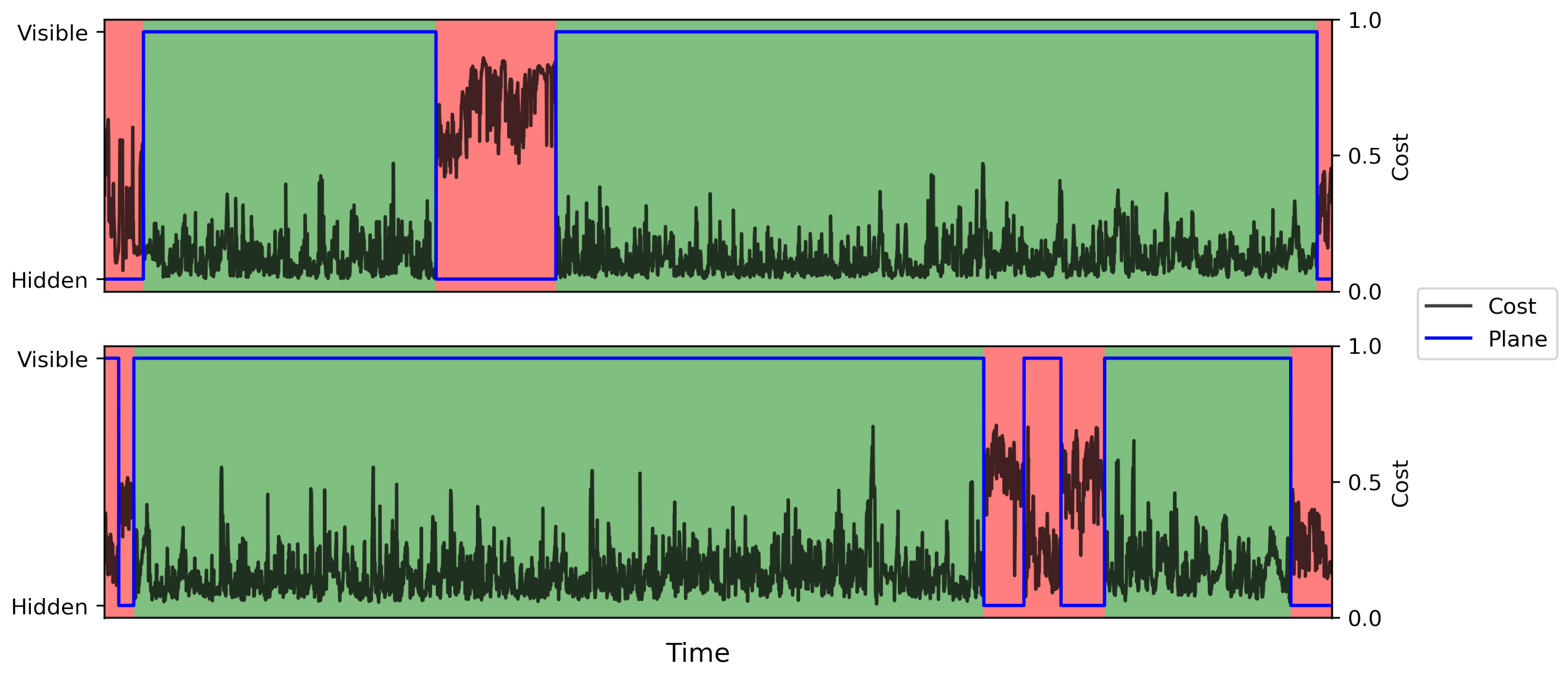
Figure 5 shows two example HSTW alignments from the music task that illustrate when HSTW performs well (top) and when HSTW performs poorly (bottom). The green and red regions indicate ground truth matching and non-matching regions in time (i.e., the red regions correspond to tampered operations), the blue line shows which plane (hidden or visible) each element of the optimal HSTW path is in, and the black line shows the corresponding costs in the pairwise cost matrix. We can see that HSTW correctly identified the tampered regions: it transitions from the visible plane to the hidden plane when there is tampering. In the bottom example, we can see that the matching and non-matching regions were difficult to differentiate based on pairwise cost values, which led to higher error rates compared to the speech task. Looking at the pairwise costs, the HSTW predictions are reasonable though incorrect.
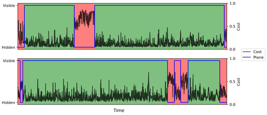
Figure 5.
Two example HSTW alignments on the music task. Green and red regions indicate ground truth matching and non-matching regions, respectively. The blue line shows the hidden/visible plane of the optimal path, and the black line shows corresponding costs in the pairwise cost matrix.
4. Discussion
In this section, we discuss the benefits of HSTW compared to previous work, its limitations, and areas of future work.
The benefits of HSTW can be viewed from two different perspectives. As mentioned earlier, alignment algorithms can be categorized into two groups: trainable alignment methods such as HMMs and parameter-free alignment methods such as DTW. Compared to trainable alignment methods, the main benefit of HSTW is its simplicity and portability: it can be easily adapted to new domains without requiring a cumbersome training process, as we demonstrated with two different tasks in this article. Compared to previous parameter-free alignment methods, the main benefit of HSTW is in its improved handling of non-matching regions (which results in an ordered partial match alignment problem). The most relevant previous parameter-free method is NWTW [20], which allows for horizontal/vertical skips as well as time warping transitions at each position in the cost matrix. While NWTW should in theory be able to handle non-matching regions as a consecutive sequence of horizontal and vertical skips, we see from Figure 2 and Figure 4 that it performed substantially worse than HSTW in handling non-matching regions. Since NWTW and HSTW both allow for the exact same types of transitions, the difference in performance comes from separating the single state (in NWTW) into two distinct states with different time warping characteristics.
There are two drawbacks to using HSTW. The first drawback is the additional computation and memory requirements compared to standard DTW. Because of the additional hidden plane in the cumulative cost matrix and backtrace matrix, HSTW requires twice as much computation and memory as DTW with the same size cost matrix. Therefore, while HSTW is in theory a generalization of DTW that could be used as a more flexible alternative, in practice its use is only recommended for handling ordered partial match alignment. The second drawback is the need to set 2–3 additional hyperparameters beyond those of standard DTW. This can be done with a very small amount of data, however, so this would be considered a relatively minor drawback. Recall that there are three hyperparameters: the skip penalty in the horizontal direction, the skip penalty in the vertical direction, and the plane transition penalty. If the alignment problem is symmetric, however, only two effective hyperparameters need to be set.
For future work, we plan to generalize HSTW to more than two states. While HSTW explores the use of a hidden and visible state, the concept can readily be extended to multiple states, each having its own time warping characteristics. This would allow one to encode structure a priori into the alignment algorithm while remaining a parameter-free algorithm.
Author Contributions
Conceptualization, T.J.T.; methodology, M.S. and T.J.T.; software, C.C., T.S., A.G., C.L. and M.S.; validation, C.C., T.S., A.G., C.L. and M.S.; writing—original draft preparation, T.J.T.; writing—review and editing, C.C., T.S., A.G., C.L. and M.S.; supervision, T.J.T.; funding acquisition, T.J.T. All authors have read and agreed to the published version of the manuscript.
Funding
This material is based upon work supported by the National Science Foundation under Grant No. 1948531.
Data Availability Statement
Non-copyrighted data for our experiments can be found at https://github.com/HMC-MIR/HSTW (accessed on 5 April 2022).
Conflicts of Interest
The authors declare that there is no conflict of interest.
Abbreviations
The following abbreviations are used in this manuscript:
| DTW | dynamic time warping |
| HSTW | hidden state time warping |
| HMMs | hidden Markov models |
| MFCCs | mel-frequency cepstral coefficients |
| ROC | receiver operating characteristic |
| kbps | kilobits per second |
| EER | equal error rate |
| NWTW | Needleman–Wunsch time warping |
References
- Sakoe, H.; Chiba, S. Dynamic Programming Algorithm Optimization for Spoken Word Recognition. IEEE Trans. Acoust. Speech Signal Process. 1978, 26, 43–49. [Google Scholar] [CrossRef] [Green Version]
- Itakura, F. Minimum Prediction Residual Principle Applied to Speech Recognition. IEEE Trans. Acoust. Speech Signal Process. 1975, 23, 67–72. [Google Scholar] [CrossRef]
- Salvador, S.; Chan, P. FastDTW: Toward Accurate Dynamic Time Warping in Linear Time and Space. In Proceedings of the KDD Workshop on Mining Temporal and Sequential Data, 2004; Available online: https://www.researchgate.net/publication/220520264_The_third_SIGKDD_workshop_on_mining_temporal_and_sequential_data_KDDTDM_2004 (accessed on 5 April 2022).
- Müller, M.; Mattes, H.; Kurth, F. An Efficient Multiscale Approach to Audio Synchronization. In Proceedings of the International Conference on Music Information Retrieval (ISMIR), Victoria, BC, Canada, 8–12 October 2006; pp. 192–197. [Google Scholar]
- Prätzlich, T.; Driedger, J.; Müller, M. Memory-Restricted Multiscale Dynamic Time Warping. In Proceedings of the IEEE International Conference on Acoustics, Speech, and Signal Processing (ICASSP), Shanghai, China, 20–25 March 2016; pp. 569–573. [Google Scholar]
- Tsai, T. Segmental DTW: A Parallelizable Alternative to Dynamic Time Warping. In Proceedings of the IEEE International Conference on Acoustics, Speech and Signal Processing (ICASSP), Toronto, ON, Canada, 6–11 June 2021; pp. 106–110. [Google Scholar]
- Zhang, Y.; Glass, J. An Inner-Product Lower-Bound Estimate for Dynamic Time Warping. In Proceedings of the 2011 IEEE International Conference on Acoustics, Speech, and Signal Processing (ICASSP), Prague, Czech Republic, 22–27 May 2011; pp. 5660–5663. [Google Scholar]
- Keogh, E.; Wei, L.; Xi, X.; Vlachos, M.; Lee, S.H.; Protopapas, P. Supporting Exact Indexing of Arbitrarily Rotated Shapes and Periodic Time Series under Euclidean and Warping Distance Measures. VLDB J. 2009, 18, 611–630. [Google Scholar] [CrossRef]
- Rakthanmanon, T.; Campana, B.; Mueen, A.; Batista, G.; Westover, B.; Zhu, Q.; Zakaria, J.; Keogh, E. Searching and Mining Trillions of Time Series Subsequences under Dynamic Time Warping. In Proceedings of the ACM SIGKDD International Conference on Knowledge Discovery and Data Mining, Beijing, China, 12–16 August 2012; pp. 262–270. [Google Scholar]
- Li, J.; Wang, Y. EA DTW: Early Abandon to Accelerate Exactly Warping Matching of Time Series. In Proceedings of the International Conference on Intelligent Systems and Knowledge Engineering, Nanjing, China, 24–26 November 2007. [Google Scholar]
- Srikanthan, S.; Kumar, A.; Gupta, R. Implementing the Dynamic Time Warping Algorithm in Multithreaded Environments for Real Time and Unsupervised Pattern Discovery. In Proceedings of the 2011 2nd International Conference on Computer and Communication Technology (ICCCT-2011), Allahabad, India, 15–17 September 2011; pp. 394–398. [Google Scholar]
- Shabib, A.; Narang, A.; Niddodi, C.P.; Das, M.; Pradeep, R.; Shenoy, V.; Auradkar, P.; Vignesh, T.; Sitaram, D. Parallelization of Searching and Mining Time Series Data using Dynamic Time Warping. In Proceedings of the IEEE International Conference on Advances in Computing, Communications and Informatics (ICACCI), Kochi, India, 10–13 August 2015; pp. 343–348. [Google Scholar]
- Sart, D.; Mueen, A.; Najjar, W.; Keogh, E.; Niennattrakul, V. Accelerating Dynamic Time Warping Subsequence Search with GPUs and FPGAs. In Proceedings of the IEEE International Conference on Data Mining, Sydney, NSW, Australia, 13–17 December 2010; pp. 1001–1006. [Google Scholar]
- Wang, Z.; Huang, S.; Wang, L.; Li, H.; Wang, Y.; Yang, H. Accelerating Subsequence Similarity Search Based on Dynamic Time Warping Distance with FPGA. In Proceedings of the ACM/SIGDA International Symposium on Field Programmable Gate Arrays, Monterey, CA, USA, 11–13 February 2013; pp. 53–62. [Google Scholar]
- Tralie, C.J.; Dempsey, E. Exact, Parallelizable Dynamic Time Warping Alignment with Linear Memory. In Proceedings of the International Conference for Music Information Retrieval (ISMIR), Montreal, QC, Canada, 11–16 October 2020; pp. 462–469. [Google Scholar]
- Macrae, R.; Dixon, S. Accurate Real-time Windowed Time Warping. In Proceedings of the International Conference on Music Information Retrieval (ISMIR), Utrecht, The Netherlands, 9–13 August 2010; pp. 423–428. [Google Scholar]
- Dixon, S. Live Tracking of Musical Performances Using On-line Time Warping. In Proceedings of the 8th International Conference on Digital Audio Effects, Madrid, Spain, 20–22 September 2005; pp. 92–97. Available online: http://www.eecs.qmul.ac.uk/simond/pub/2005/dafx05.pdf (accessed on 5 April 2022).
- Fremerey, C.; Müller, M.; Clausen, M. Handling Repeats and Jumps in Score-Performance Synchronization. In Proceedings of the International Conference on Music Information Retrieval (ISMIR), Utrecht, The Netherlands, 9–13 August 2010; pp. 243–248. [Google Scholar]
- Shan, M.; Tsai, T. Improved Handling of Repeats and Jumps in Audio-Sheet Image Synchronization. In Proceedings of the International Society for Music Information Retrieval (ISMIR), Montreal, QC, Canada, 11–16 October 2020; pp. 62–69. [Google Scholar]
- Grachten, M.; Gasser, M.; Arzt, A.; Widmer, G. Automatic Alignment of Music Performances with Structural Differences. In Proceedings of the International Society for Music Information Retrieval Conference (ISMIR), Curitiba, Brazil, 4–8 November 2013. [Google Scholar]
- Müller, M.; Appelt, D. Path-Constrained Partial Music Synchronization. In Proceedings of the International Conference on Acoustics, Speech, and Signal Processing (ICASSP), Las Vegas, NV, USA, 31 March–4 April 2008; pp. 65–68. [Google Scholar]
- Müller, M.; Ewert, S. Joint Structure Analysis with Applications to Music Annotation and Synchronization. In Proceedings of the International Society for Music Information Retrieval Conference (ISMIR), Philadelphia, PA, USA, 14–18 September 2008; pp. 389–394. [Google Scholar]
- Waloschek, S.; Hadjakos, A. Driftin’ Down the Scale: Dynamic Time Warping in the Presence of Pitch Drift and Transpositions. In Proceedings of the International Conference on Music Information Retrieval (ISMIR), Paris, France, 23–27 September 2018; pp. 630–636. [Google Scholar]
- Wang, S.; Ewert, S.; Dixon, S. Robust and Efficient Joint Alignment of Multiple Musical Performances. IEEE/ACM Trans. Audio Speech Lang. Process. 2016, 24, 2132–2145. [Google Scholar] [CrossRef]
- Sapp, C. Hybrid Numeric/Rank Similarity Metrics for Musical Performance Analysis. In Proceedings of the International Conference for Music Information Retrieval (ISMIR), Philadelphia, PA, USA, 14–18 September 2008; pp. 501–506. [Google Scholar]
- Schreiber, H.; Zalkow, F.; Müller, M. Modeling and Estimating Local Tempo: A Case Study on Chopin’s Mazurkas. In Proceedings of the International Society for Music Information Retrieval Conference (ISMIR), Montréal, QC, Canada, 11–15 October 2020; pp. 773–779. [Google Scholar]
- Grosche, P.; Müller, M.; Sapp, C.S. What Makes Beat Tracking Difficult? A Case Study on Chopin Mazurkas. In Proceedings of the International Conference for Music Information Retrieval (ISMIR), Utrecht, The Netherlands, 9–13 August 2010; pp. 649–654. [Google Scholar]
- Zakariah, M.; Khan, M.K.; Malik, H. Digital Multimedia Audio Forensics: Past, Present and Future. Multimed. Tools Appl. 2018, 77, 1009–1040. [Google Scholar] [CrossRef]
- Chesney, B.; Citron, D. Deep Fakes: A Looming Challenge for Privacy, Democracy, and National Security. Calif. L. Rev. 2019, 107, 1753. [Google Scholar] [CrossRef] [Green Version]
- Needleman, S.B.; Wunsch, C.D. A General Method Applicable to the Search for Similarities in the Amino Acid Sequence of Two Proteins. J. Mol. Biol. 1970, 48, 443–453. [Google Scholar] [CrossRef]


Publisher’s Note: MDPI stays neutral with regard to jurisdictional claims in published maps and institutional affiliations. |
© 2022 by the authors. Licensee MDPI, Basel, Switzerland. This article is an open access article distributed under the terms and conditions of the Creative Commons Attribution (CC BY) license (https://creativecommons.org/licenses/by/4.0/).