Article

Effect of Dimensional Variables on the Behavior of Trees for Biomechanical Studies

1
Structural Wood Engineering Platform, University of Santiago of Compostela, Benigno Ledo Street, 2, 27002 Lugo, Spain
2
School of Agricultural Engineering, University of Campinas, Cândido Rondon Avenue, 501, Cidade Universitária, Campinas, São Paulo 13083-970, Brazil
*
Author to whom correspondence should be addressed.
Appl. Sci. 2022, 12(8), 3815; https://doi.org/10.3390/app12083815
Submission received: 28 February 2022 / Revised: 24 March 2022 / Accepted: 25 March 2022 / Published: 10 April 2022
(This article belongs to the Special Issue Recent Advance in Finite Elements and Biomechanics)

Abstract

:
The dimensional variables of trees play an important role in biomechanical studies that seek to estimate the risk of falls, since they influence their biomechanical behavior in relation to the forces to which they are subjected, and therefore, their safety factor. The aim of this research is to evaluate the effect of dimensional variables of trees on their mechanical behavior. A finite-element model was used to perform linear static analysis. The wood from the tree was considered clean, and the architectural model was based on dimensional variables of species commonly used in urban afforestation in São Paulo, Brazil. Different slenderness, tapering, height, and load level were used to analyze the tree mechanical behavior. The numerical-simulation model facilitates the evaluation of the influence of dimensional parameters of trees on deflections and stresses. The behavior of the deflections varies according to height, diameter, and loading level. Since the model considers the geometric variations of the section, the stresses show smooth variations along the trunk. The maximum module values of positive and negative stresses are not equal, and can undergo sudden variations in position along the trunk when local maximum stresses become global maximums.

1. Introduction

In biomechanics studies, it is customary to apply known theories of mechanics developed for conventional structures, including many limitations to represent the plant’s behavior [1,2]. Some of these limitations are the use of equations that are only valid for small deflections and static equations for analyzing the wind load, which is dynamic [1,3]. Wood and most plant materials are viscous and therefore have a nonlinear behavior, making theory and reality not coinciding [2]; even so, the studies are valid, so it is possible to obtain approximations. Another significant limitation is the isotropy of the material, as cited by [1]. This can be minimized with the use of models that allow the application of the orthotropic condition; however, to circumvent this limitation, it is necessary to know the complete elastic parameter of the wood.
The safety factor is another limitation related to applying theories of conventional mechanics in trees. For conventional structures, the safety factor is usually considered the relationship between the load capacity and the acting load [4]. This proportion must be greater than or equal to one for the structure to be reliable. However, many publications indicate that plants are structures that withstand stresses much higher than those expected by the conventional design resistance [5,6,7,8,9] Proposals for measurements of plant safety factors have been developed through studies of the relationship between breakdown and expected service stresses in situations of applied external forces [9]. Thus, the safety factors of trees reported in the literature are generally based on studies applying static loads [8], such as pulling tests. In ref. [10] showed that the safety factors in the trees vary sinusoidally, so that the smallest safety factors occur for peripheral branches and the lower parts of the trunk. As such, the intermediate parts of the tree have significantly greater safety factors. According to the authors, this is a tree strategy so that the branches break first, reducing the crown, and thus reducing the drag forces acting on the trunk, especially in the intermediate parts where the maximum stresses are expected. The literature suggests that trees could withstand stresses three to five times higher than other wooden structures without breaking [5,6,7,8,10,11]. In addition, the wood strength obtained in tests using specimens is not compatible with the stresses supported by the tree trunk, even within the limit of proportionality [12,13], making field trials with whole trees important.
In addition to the limitations related to the theories of mechanics, there are many others related to the material of live trees. Some worth mentioning are the differences in rupture for dry and physiologically inactive wood [14], great capacity to undergo deflections much higher than the elastic-band linear [14], complex geometry, great adaptive ability to respond to external stimuli, as well as changes due to the formation of different types of wood [1].
Although the representation of the wind as static horizontal loads (even though they are dynamic) [15] simplifies the analysis and makes it more accessible, it can introduce some inaccuracies [1,2,3]. In ref. [16] shows that the maximum inclination of the root zone of the structure measured by the static-pulling test was 68% lower than the one obtained with natural wind, demonstrating that the static analysis can underestimate the tree’s response. In ref. [17] also reported that their results show that trees fell with wind speeds 56% lower than the critical speed values obtained through the traction test. The finite-element method (FEM) can be used to study the dynamic behavior of a structure, but this approach is more complex, involving inertial-mass forces, elastic forces, and damping forces, whereas static analysis considers only the elastic forces [1,18]. The dynamic response of the tree is important, but the wind load is also important and quite complex to model, requiring accurate empirical measurements of many parameters of the tree and load conditions to obtain reliable results [1,18]. Despite knowing the limitations and errors, static analyses to simulate the wind are still performed due to the inherent difficulties of dynamics analyses. In addition, it is important to note that the oscillation induced by the wind load alters the effort produced in the trunk, sometimes reducing it, and this favorable condition is not considered when using horizontal loads to simulate the wind [1,3,19]. Furthermore, dynamic loads are short-term loads, while static loads are relatively long-term [1]. These two aspects (canopy movement and short-term load) can play a favorable role in reducing the load transmitted to the trunk and improving the response of the wood, respectively, indicating that static analysis will not always underestimate the results. New results using the digital-image-correlation system (DIC) may be a future way of mapping strains in standing trees, even on complex tree surfaces, allowing for the simplification of dynamic analysis in biomechanical studies on trees [18].
Static-load tests using a cable attached to the tree to apply a controlled tension (pulling test) have been widely used to induce nondestructive bending stress in the linear elastic range and thus extrapolate the critical-bending moment. In ref. [12] shows that the material properties determined in small specimens are less relevant for evaluating tree strength than values derived from the test of whole tree stems, indicating that despite the limitations, static-field methods are important tools to be used in biomechanical studies. However, this test does not consider that plastic deformations frequently occur in live trees, increasing their carrying capacity [1]. This test is also used to estimate the resistance to uprooting by models, relating the bending moments necessary to induce small changes in the slopes of the soil–root plate. These models are used to extrapolate failure loads but have been criticized because the angle of rotation of the root plate at maximum strength varies with the age of the tree, root architecture, and soil structure [1]. In ref. [17] concluded that it is necessary to solve some problems related to the pulling-test equipment and that further research is needed to know the drag coefficient, the pedohydraulic condition of the soil, and the relationship between static and dynamic conditions. Some authors, cited in the review by [1], show that static-load tests will advance by using optical digital 3D-image correlation (DIC) to measure strain and stress in branches, trunks, and roots, allowing further studies in bending, torsion, and fracture in woody plants and further in-depth understanding of strain during static-load tests, allowing consideration of the impact of plastic deformations. Refs. [19,20,21] are examples of the incorporation of DIC in static-pulling tests. Both researchers show that the DIC method can be used successfully to obtain high-quality strain data in tensile tests.
In addition to research aimed at obtaining improvements in static-field tests, researchers have been studying ways to use numerical models to identify parameters that mainly impact the response of trees [22] and estimate the distribution of deformations and stresses along the trunks of trees exposed to gravitational and horizontal loads [23,24]. These models can help evaluate the effects of the architectural characteristics of the roots and soil properties on the distribution of loads around the root system [25] as tools in analyzing tree ruptures [26]. They can also help in the study of the influence of a series of parameters (mechanical properties and geometry of the root system and the stem) on stress, strain, and displacement of the tree model [24]. Numerical models are also being studied to represent the branches [27] better and to simulate the dynamics of the tree [28], and to uproot with wood-breaking behavior [29].
The dimensional variables of the trees (base diameter, diameter at breast height (DBH), height, length of branches, etc.) can be measured directly. Thus, in addition to being an important tool for the forestry industry, the simplicity of its measurement can be a valuable tool to assess the risk of falling urban trees in biomechanical analyses, including through numerical models. Geometry and stem dimensions significantly affect the dynamic response [30] and stresses, strain, and displacements [24] of trees subjected to wind loads than their wood properties. These authors also concluded that nonlinear behaviors are a function of the architecture of the branches. Considering that wind is the most critical load in analyzing fall risk [1,31], this result indicates the importance of tree dendrometry. In predictive models for falls, it is important to know not only the mechanical characteristics of the stem and branches, but also the dimensions and shape of the trees [1,22,31,32,33].
The objective of this research was to evaluate, through numerical simulation, the effect of dimensional tree variables on deflection and normal and shear stresses and to discuss the consequences on the safety factor of trees.

2. Materials and Methods

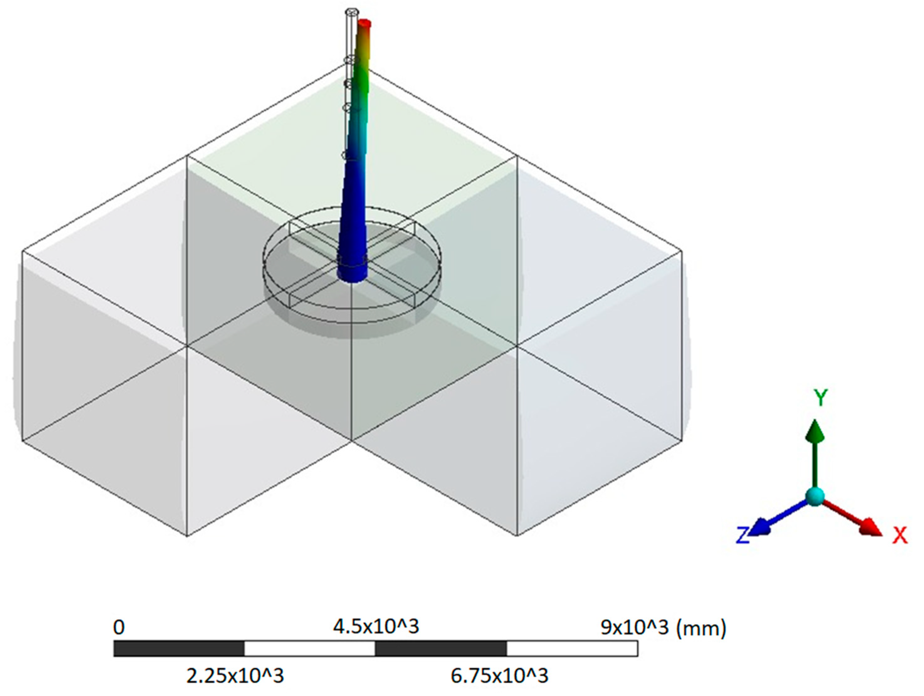
2.1. Finite-Element Model

The dendrometric characteristics of the trees, such as height, slenderness, and taper, play an essential and complex role in the risk of falling trees. Therefore, to make more viable the analysis of the influence of these dendrometric parameters in the deflection and in normal and shear stresses, this study proposed to create a numerical modeling using the finite-element method (FEM). The model was developed using the Ansys® Academic Research Mechanical, Release 18.2 software. The system was composed of the trunk, root, and soil bin (Figure 1). The FEM model was created using a mesh with solid and quadratic 3D elements (Figure 1), varying in number according to the size of the tree and the type of element (trunk, root, or soil bin), with a maximum size of 200 mm for the tree and 300 mm for the soil bin. The displacement and stress fields are computed considering the linear static analysis.
The root was simulated as a 0.15 m deep disc, as proposed by [34]. The root diameter varied according to the crown. The crown diameter varied according to the tree’s height and was fixed at 5.5 m in the scenario where the height is fixed. The soil bin proposed by [26] also had a fixed dimension (16 m × 16 m), but in our model, the cubic-shape soil bin was simulated with a dimension proportional to the root (2.62 times). In addition, as proposed by [26], frictions between soil and root were ignored, and for boundary conditions, only the base was considered fixed. The trunk (without crown and branches) was created as conical (larger at the bottom) instead of cylindrical, as proposed by [10] (Figure 1).
To propose the tree model (architecture) and the range of the dimensions of the trunk and branches, we used some results from [35] as a reference. The study [35] was carried out with six species of trees (Handroanthus pentaphylla (Ipê Rosa), Cenostigma pluviosum (Sibipiruna), Tipuana tipu (Tipuana), Schinus molle (Aroeira Salsa), Caesalpinia ferrea (Pau Ferro), and Schinus terenbinthifolius (Aroeira pimenteira), which are all commonly planted in the state of São Paulo, Brazil.
As the proposed model uses only the conical trunk (without canopy), it was necessary to consider, in a simplified way, the effect of the branches and leaves. Thus, the weight of branches and leaves was considered as a concentrated load at the end of the branch, allowing the calculation of a moment, which was applied to the trunk. To obtain reference data for calculating the weight of branches, we also used the results (diameter, length, tapering, and density of tree branches) obtained in previous research [3,35]. We added 4.0% of the weight of the branch to consider the weight of the leaves, as proposed by [36]. The mean value of calculated moments (969 N·m) was applied at three levels, representing the most common tree architecture obtained in the previous study [35]. The height levels varied according to the total height of the tree (Table 1). The first level was always at the first fork (the point where the canopy begins), which was set at 2.0 m (average value obtained in [35]). From that point, the canopy height (H-h) was divided into three parts to place the remaining levels of branches (Table 1). For each level, four branches were adopted around the trunk: two in the X direction, with moments around Z; and two in the Z direction, with moments around X (Figure 1). Moments on opposite faces were considered with opposite signs (X1 positive and X2 negative and Z1 positive and Z2 negative).
A reference density (994 kg·m−3) for trunk wood, obtained in [35], was introduced in the FEM model to calculate the trunk self-weight.
Three scenarios were proposed to evaluate the effect of dimensional variables on the behavior of trees subjected to moments, gravitational and horizontal loads. In the first scenario, total trunk height (H) varied while slenderness (l) and taper (T) values were fixed (Table 1). In the second scenario, l varied while H and T values were set, and, finally, in the third scenario, T varied while H and l values were fixed (Table 1).

2.2. Horizontal Load

For simplification purposes, the dynamic wind loads given by the wind pressure (q) were transformed into a horizontal load (PHV) (Equation (1)), applied to the center of gravity of the crown. This simplification is common in the literature [3].
P H V = q A c
where Ac is the area of the front surface of the crown.
Wind pressure (q) depends on air density (ρ) and wind speed (V) according to Equation (2).
q = ½ ρ V 2
Assuming that the air density is approximately 1225 kg·m−3 (at sea level and 15 °C) and considering the acceleration of gravity (m·s−2), the value of the wind pressure (q in N·m−2) is obtained (Equation (3)).
q = 0.613   V 2
Therefore, horizontal loads depend on wind pressure and canopy area (Equation (1)). The wind pressure depends on the wind speed, while the crown area depends on the size and architecture of the crown. As [35] shows that the most common tree architecture was the monopodial shaped like a globose (round) crown, the crown was simplified to a circumference (Figure 1) with a diameter equal to the height of the tree minus the height of the first fork assumed in this work as the average value obtained by [35], which was two meters.
Assuming a range of wind speeds, we also obtain a range of wind pressures (Equation (3)) and, therefore, horizontal loads (Equation (1)). We started the procedure testing a range of wind speeds covering speeds below, within, and above basic wind speeds (peak gust speed averaged over a short time interval of about 3 s duration and measured at 10 m above ground) used in the Brazilian standard, [37] which are 30 m·s−1 to 50 m·s−1. We calculated the wind pressure (Equation (2)) using this wind-speed range (from 30 m·s−1 and 50 m·s−1), and the horizontal load (Equation (1)) was calculated, with frontal canopy area (Ac in Table 2). As we need to apply the same horizontal load to all scenarios (Table 1), the second analysis was to use the horizontal-load range (obtained for the different areas of canopy) to calculate the respective wind pressure (Equation (1)) and so the respective wind speeds capable of producing this level of load (Equation (3)). Since below 5 kN and above 15 kN the wind speed was, respectively, far below (for the largest canopy) and far over (for scenario 1) the proposed wind-speed range, we choose the three load levels (5 kN, 10 kN, and 15 kN) to be applied to all scenarios. According to the Beaufort scale, at speeds from 5.5 to 7.9 m·s−1 the wind moves small branches; from 8 to 10.7 m·s−1 it moves large branches and small trees; from 13.9 to 17.1 m·s−1 it moves large trees; from 17.2 to 20.7 m·s−1 it can break branches; from 20.8 to 24.4 m·s−1 it can damage trees; and from 24.5 m·s−1 it can uproot trees. The chosen load levels allow us to simulate wind speeds from 4.4 m·s−1 to 58.8 m·s−1 (Table 2), but with the exception of trees with H = 5 m where the speeds are greater than 30 m·s−1, all other conditions are simulating at speeds below 22 m·s−1 (Table 2), i.e., in the range where large tree damage is not expected by the Beaufort scale. Furthermore, for shorter trees, greater stability is expected due to their lesser slenderness, and, therefore, these short trees will likely be better able to withstand greater wind forces. The same wind-speed level was used by [10], for example, who simulated wind speeds of 10, 20, and 50 m·s−1.
These horizontal loads were applied to the tree model in a position coincident with the gravitational center of the crown (Table 1).

2.3. Material Properties

Soil was considered isotropic, and the values obtained by [34] were adopted (Density = 1730 kg·m−3, Modulus of Elasticity = 13.5 MPa and Poisson’s ratio = 0.4).
The trunk and root wood were considered orthotropic, and the values adopted in the simulations were the average physical and mechanical properties in the saturated condition, studied in the research group via ultrasound test in polyhedral specimens. This methodology [38,39] allows us to obtain, with ultrasound, the stiffness matrix and the inversion, the compliance matrix; therefore, the nine elastic constants of the wood (three longitudinal moduli, three shear moduli, and six Poisson’s ratio). Thus, for the numerical simulation, considering the material’s orthotropy, three elasticity moduli (longitudinal (EL), radial (ER), and tangential (ET)); three shear moduli in the planes (GRT, GLT, and GLR); and three Poisson’s ratio in the planes (νLR, νLT, and νRT) are inserted. In general, elastic constants of wood determined by elasticity theory consider the longitudinal direction as X, the radial direction as Y, and the tangential direction as Z. We use this same terminology for the local coordinate system. In the complete characterization of this material, six Poisson’s ratio were obtained (νRL, νTL, νLR, νTR, νLT, and νRT) (Table 3). However, the FEM only allows the incorporation of three values, as it uses reciprocal relationships internally (Equation (4)):
ν T L E T = ν L T E L ;   ν R L E R = ν L R E L ;   ν R T E R = ν T R E T
Given that the νRL and νTL Poisson’s ratio are the lowest (Table 3) and in practice are obtained with less experimental precision, the calculations were performed, providing the program with the values of νLR (0.49) and νLT (0.64). In the case of the RT plane, we followed the same logic, using the highest value (νRT = 0.78).
Although the model allows the use of different properties for root and trunk, the same values (Table 3) were used for both because we had no properties available for root.

2.4. FEM Simulation

With the simplified topology adopted (Figure 1) and the wood parameters (Table 3), for each scenario (Table 1), the deflection and normal (parallel to fiber) and shear (LR plan) stresses (positives and negatives), as well as the position of these values along the trunk, were obtained, using the FEM (Ansys R18.2). The FEM simulation model used in this paper considers the deflection of all systems (root-plate and stem) (Figure 2).

2.5. Safety Factors

For all scenarios, safety factors were analyzed using the traditional expression for structures (relation between load-bearing capacity and active load).
The active loads were obtained in FEM simulations (maximum normal and shear stresses), and the load-bearing capacity using average strength data in saturated condition obtained by associating the strength classes of the European Standard [40] to EL, obtained as mentioned previously (Table 3). For this association, we corrected the EL obtained in saturated conditions (Table 3) to the reference moisture content (12%) using the European Standard [41] (1% for each 1% variation around the reference value up to 20%) and used the value of corresponding strength (fm,k = 39 MPa). The relations proposed in the European standard [41] were also used to infer the characteristic shear strengths (fv,k = 0,2 (fm,k)0.80 = 3.8 MPa). The [42] was used to determine the design values (Equation (5)), considering the modification coefficient (kmod) for solid wood, class of service 3 (totally exposed directly to rainwater and climatic conditions), and short-term loading class (permanent + wind), resulting in kmod = 0.70. For the partial safety coefficient, γm = 1.3 (solid wood) was used.
f w , d = k m o d f w , k γ m
where: fw,d = design resistance; kmod = modification coefficient; and γm = partial safety coefficient.
Thus, considering engineering parameters applied to conventional wooden structures, the design resistance, using strength in the saturated condition, was inferred in bending (fm,d = 21 MPa) and shear (fv,d = 2 MPa). With the design resistances considered as load-bearing capacity in bending and in shear as well as the acting forces (normal and shear stress) obtained from the simulations, the safety factors for all scenarios were calculated and discussed based on the specific behavior of the trees presented in the literature.

3. Results and Discussion

3.1. Deflection

3.1.1. Comparison with Literature

Comparing deflection values using literature is complex because different authors use different measurement methodologies. Some of them consider only the inclination of the root plate [15,17], and others consider the inclination of the root plate and the deflection of the stem together [26,33,43], as in this study (Figure 2). Furthermore, the deflection is influenced by geometric tree parameters such as height, diameter, and taper [24], and also by mechanical properties of the trunk and root wood, as modulus of elasticity [15]. Therefore, the comparison with literature is focused on the analysis of the general order of magnitude of the values obtained and the coherence of behavior, considering geometric parameters of the trees and properties of the wood adopted by different authors.
In ref. [43] uses two trees with the same height (H = 20 m) and diameters at breast height (DBH = 24.5 cm and 24.8 cm), both same species with density 300 kg·m−3 and modulus of elasticity in bending 3584 MPa. The horizontal pulling force, with a magnitude much lower (maximum 2.25 kN and 1.65 kN) than those used in this research (5 kN to 15 kN), was applied at 12.23 m and 12.20 m (about 60% H). The closest condition to compare our data is in scenario 1, where the tree with H = 20 m (Table 1) was subjected to a horizontal load of 5 kN at 55% H (Table 4). For a horizontal load of 1.65 kN, the average displacement at the point of load application obtained by [43] was 1.5 m. If we apply a composition of differences of DBH (24.7 cm/91 cm = 0.27) and modulus of elasticity (3584 MPa/10387 MPa = 0.34) calculated by multiplying these differences (0.09), the expected displacement (0.14 m) will be of the same order of magnitude as those obtained in this paper (0.293 m in Table 4).
In ref. [34] simulated a tree with H = 8 m, DBH = 0.40 m, and horizontal force applied at 5 m (62.5% H). The simulated horizontal forces ranged from 5 kN to 75 kN. There is no information about the modulus of elasticity of the stem and root used in the model. The closest condition in this research is in scenario 2 for slender = 16, where H = 7.5 m and DBH = 0.47 m (Table 1) with horizontal load applied at 63.3% H. For this condition, the deflection in the horizontal-load position was 0.027 m (horizontal load = 5 kN (Table 4)), 0.028 m (horizontal load = 10 kN (Table 5)), and 0.029 m (horizontal load = 15 kN (Table 6)). For these load levels, [34] obtained 0.02 m, 0.03 m, and 0.04 m, with the same order of magnitude as our results.
In ref. [33] modeled, using the structural theory of a cantilever beam, the behavior of eight trees with H ranging from 9.6 m to 13.2 m subjected to large deflections using a pulling test. The modulus of elasticity of the trees’ wood was 2000 to 6400 MPa, and the diameter (D) was measured at 2 m from the base of 10 cm to 19.2 cm. The horizontal load was applied at about 70% H. The deflection of the trees ranged from 2 m to 6 m and showed positive dependence on the modulus of elasticity and diameter. The mean deflection of two trees (H = 9.6 m, DBH = 15.5 cm, and modulus of elasticity = 4000 MPa) tested by [33] is 2.5 m. We calculated a factor to compare the tree in our scenario 2 (H = 10 m, DBH = 45 cm and modulus of elasticity = 10,387 MPa and horizontal load applied at 60% H) by multiplying the diameter ratio (0.34) and modulus of elasticity ratio (0.39) and the expected deflection is 0.33 m for these trees. This value is on the same order of magnitude as that obtained by the model proposed in this paper (0.57 m).
The results of the comparisons show that although at first glance, the deflections obtained with the proposed model are very small, the values obtained by adjusting the diameter and modulus of elasticity are within the expected order of magnitude.

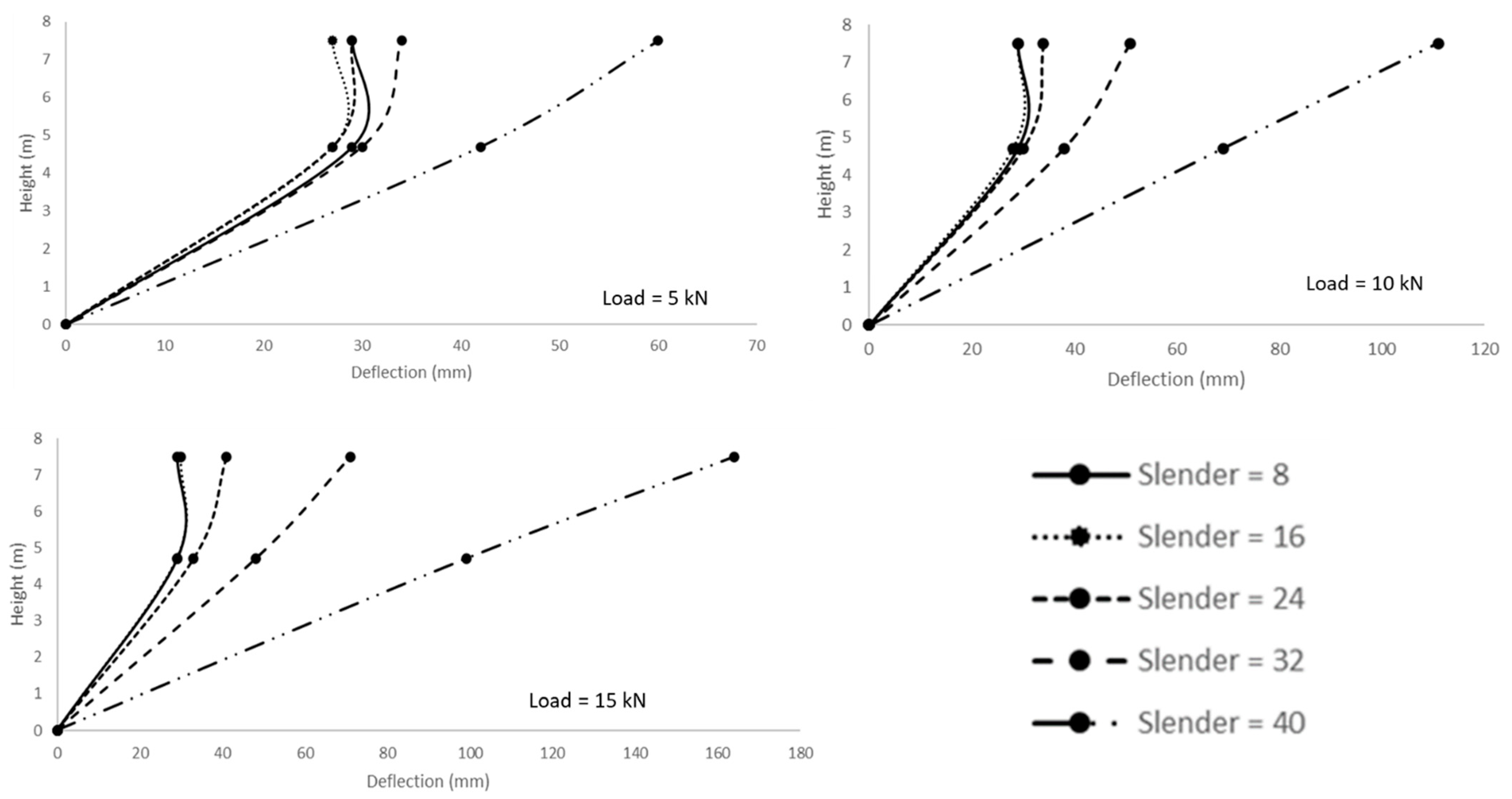
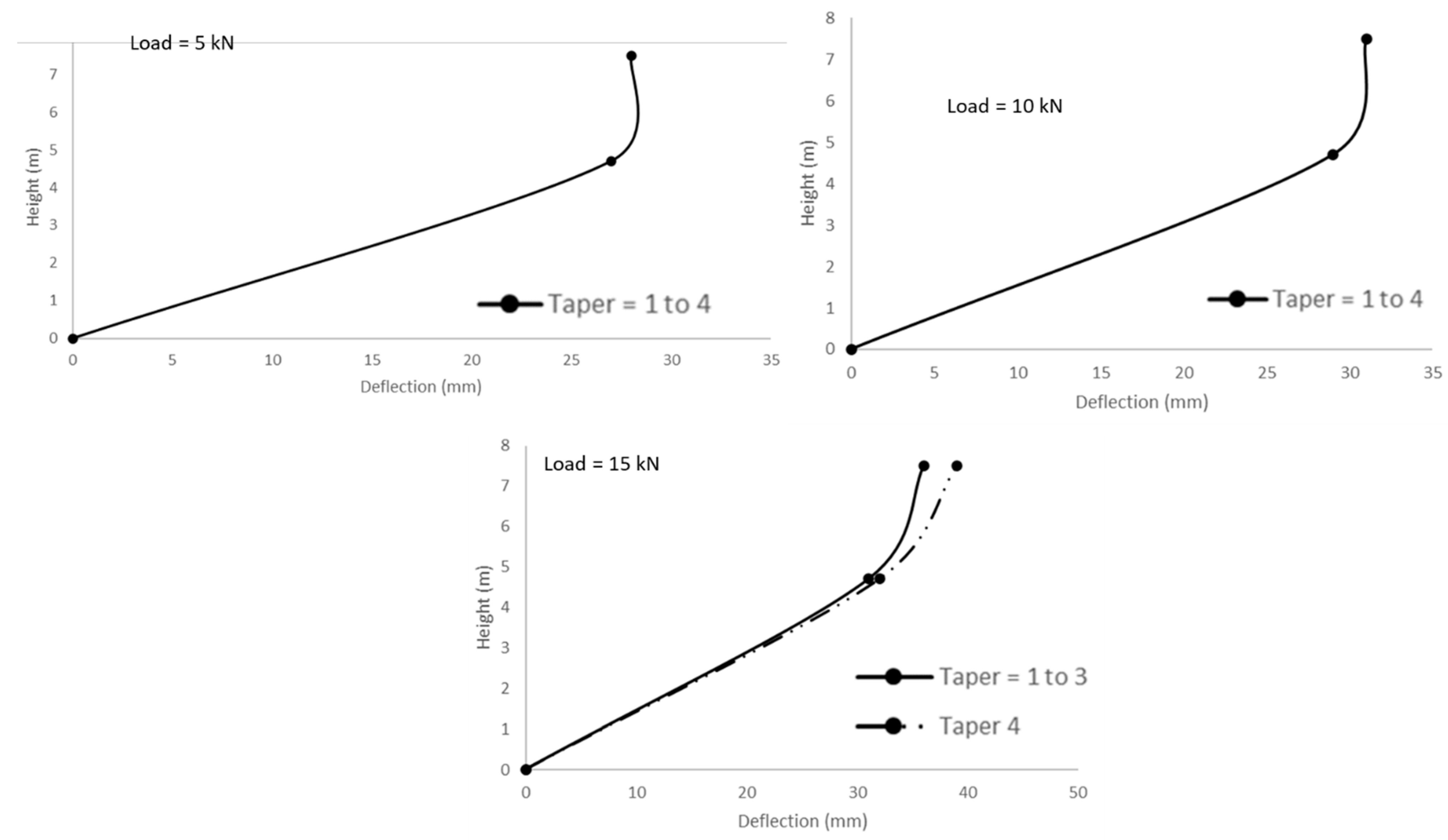
3.1.2. Behavior of Trunk Deflection with Tree Height

The deflection calculated by the model (Table 4, Table 5 and Table 6) is complex because it involves root-plate and trunk deflection under the interactions of self-load, horizontal load (simulating wind), and moments (simulating the branches’ effect). The trunk self-load only causes compression stress if the trunk is in a vertical position, but with the deflection of the trunk, this self-load will also have a horizontal component that will add bending. Moments representing branches also increase bending above the first bifurcation, and part of these moments are acting above the horizontal load position. Horizontal load causes bending of the trunk below this point, which is proposed as the center of gravity of the canopy. In a simplified way, until the break an increasing linear deflection with the height from the base to the top of the trunk is expected, but as the deflection is due to all load components in addition to the variation in dendrometric characteristics (conical trunk), this was not the behavior obtained for all scenarios.
In scenario 1, only the smaller tree (H = 5 m) showed increasing deflection with the tree’s height to the top (from 0%H to 100%H) (Figure 3). Independent of the load level, deflection values in scenario 1 for trees with a height of 10 m to 25 m show deflections at the top (dM) very similar (≥95%) or even equal to those at the point of horizontal-load application (dL), maintaining the line practically constant for the section above the point of application of the horizontal load (Figure 3). For the smaller tree (H = 5 m), the differences between the deflection at the top and at the horizontal-load point increase as the load level increases (horizontal-load position 76.9% of the top position for 5 kN horizontal load, 72.7% for 10 kN horizontal load, and 67.7% for 15 kN horizontal load) (Table 4, Table 5 and Table 6). This behavior is probably related to the association of the magnitude of the top diameter and the concentration of moments arising from the branch effect. In taller trees, the diameters are greater than about 0.2 m (Table 1), and as the position of the first bifurcation is fixed at 2 m, the height of the canopy increases with increasing tree height, and thus increasing the distance from the points of the trees where moments are applied, reducing its concentration in the canopy.
In scenario 2, the differences between the deflection in the horizontal-load position and the top position increase with increasing slender, and are influenced by the load level (Figure 4). For the first load level (5 kN), the only tree with l = 40 has the deflection growing from the base to the top. As the load level increased to 10 kN and 15 kN, this behavior started to be observed in the tree with l = 32 and l = 24, respectively (Figure 4). The slender is related to the height of the tree and the diameter at breast height, which is associated with the diameter of the top (conical trunk). In this scenario, the tree’s height is fixed (7.5 m), so the distance of the moments from branches is also fixed. The most significant differences of deflection at the top and the horizontal load point came from top diameters less than 0.127 m (above slender = 24, Table 1).
In scenario 3, as in scenario 2, the height of the tree is fixed (7.5 m); all conditions have the same moment concentrations, but the top diameter decreases as the taper increases, and as in the other two scenarios, more significant differences are obtained for the smaller top diameter. Up to 10 kN load level, the behavior is the same for all taper levels, keeping the deflection line practically straight for the section above the horizontal-load-application point (Figure 5). The behavior in scenario 3 started to change to load = 15 kN.
In ref. [33] presents graphics of stem deflection at different heights for eight trees showing variation in the slope of the curve from the point of application of the horizontal load, which in some trees is also straighter.
In the European Standard [44] focused on timber design, the maximum instantaneous deflection allowed for the cantilever condition, used to represent the condition of trees, is the length of the piece (L) by 150 or 250. For heights above 15 m in scenario 1 for all loading levels (Table 4, Table 5 and Table 6), the deflection was not compatible with this limit. However, it is important to remember that these limits, set by timber design standards, are only a reference, as the plants have an adaptive capacity that makes them capable of deforming well beyond the usual elastic limits of structures [7].

3.2. Normal Stresses

For maximum normal stresses (positive and negative) (Figure 6), the influence of slenderness is the most significant, followed by tapering. Regarding tapering, ref. [24] found stress influence for trees with heights bigger than four meters, corresponding to all of our scenarios. Height is the least influencing factor. Height variation had a small impact mainly on trees with up to 10 m (Figure 6). Statistically, height had less influence on normal negative stresses (nonsignificant regression model at all load levels), and its effect on normal positive stresses depended on the load level (Table 7).
In scenario 1, for the trees with heights ranging from 15 m to 25 m, the maximum normal stresses (positive and negative) always occurred at the base (Table 4, Table 5 and Table 6). However, for the shortest trees (5 m and 10 m), the maximum normal stresses rose to higher trunk positions, reaching more central regions (Table 4, Table 5 and Table 6). Since our model considered the tapered trunk, the geometric parameters that go into calculating the stresses varied, even though the moments generated by the horizontal load are greater at the base. In ref. [45], using mathematical models, showed that the variation in dimension and mass along the trunk influences the stress distribution. In ref. [10] simulated a 13 m tree composed of three cylindrical elements with successive diameter reduction, without branches, subjected to horizontal-static loads to simulate wind speed of 10, 20, and 50 m·s−1. The authors’ results showed that although the bending moments increased from the top to the bottom of the tree and the maximum moment was located near the base, the normal stresses varied along the stem following a third-degree polynomial. The results obtained by [33] show that the maximum normal stresses occur between 19% and 63% of the total height of the tree. The same study also shows that shortest trees had the highest maximum stress position (63% H), and the stress distribution along the trunk generally followed a fourth-degree polynomial. In ref. [46] found that uniformly tapered stems (i.e., those of Cryptomeria japonica trees) subjected to wind and snow loads had breaks located between 50% and 70% of the tree’s height, while In ref. [43] showed trunk break at 13.5% H. The distribution of stresses along the stem is influenced not only by the horizontal load considering the wind, but also by the moments applied considering the branches and by the horizontal components of the self-weight, which appear due to the deflection of the trunk. Furthermore, stresses are affected by diameter variation, which impacts the moment of inertia of the transversal section of the trunk. These loads are composed of the horizontal load, changing the behavior of the stresses along the trunk [47].
In scenario 2, to have slenderness variation keeping the height (7.5 m) and the taper (0.030) fixed, it was necessary to vary the DBH from 0.19 m to 0.94 m, reducing the maximum stresses in smaller l conditions that correspond to the highest DBH. A compilation of the results of pulling tests with more than 4500 trees carried out in ten different countries shows that, as expected, taller trees are subjected to higher wind loads (Wessolly, 2004 cited by [11]), with an increase in the resulting moment in the base. However, the stem diameter strongly influences the resulting stresses (Wessolly, 2004 cited by [11]). The maximum normal stresses (positive and negative) in this scenario range from 0% H to 63% H (Table 4, Table 5 and Table 6). Studies by [33] and [10] attribute the variation of stress along the stem to the slenderness, with a deflection from the base (where the maximum moments occur due to the action of wind forces) for the upper regions of the stem. These authors also reject the hypothesis of constant stress distribution along the stem, and conclude that such distribution is strongly dependent on the relationship between height and diameter.
In scenario 3, with defined height (7.5 m) and slenderness [22] and varied taper, normal stresses (positive and negative) grow as the tapering increases, and the position of these maximums varies from 23% H to 63% H (Table 4, Table 5 and Table 6).

3.3. Shear Stresses

The behavior of the position for maximum shear stresses along the trunk, simulated in Scenario 1 (trees of different heights), was similar to that of normal stress (Figure 7); that is, maximum stresses (positive and negative) at the base for trees ranging from 15 m to 25 m high, and in higher positions for lower trees (H = 5 m and 10 m) (Table 4, Table 5 and Table 6). In scenario 2, the maximum shear stress occurs at the base only for the minimum λ (correspondent to the maximum DBH) for all levels of load (Table 4, Table 5 and Table 6). In scenario 3, the maximum shear stresses (positive and negative) increase with taper growth, while the position of the maximum varies from 26% H to 51% H. Statistically, height had an influence on the negative shear stresses only for the lowest horizontal load (5 kN) and on the shear positive stress for the two highest horizontal-load levels (5 and 10 kN) (Table 8). Slender and tapper had a statistical influence on the shear stress for all load levels (Table 8).

3.4. General Behavior of the Stresses along the Trunk

Due to the characteristic of the applied load, which consists of some forces and moments concentrated along the trunk, the stress/strain field in the model has some local maximum stresses/strains. Therefore, as the geometric parameters change, some of these local maximum stresses/strains can become the maximum global value. Therefore, although Table 4, Table 5 and Table 6show some sudden changes in the position of the maximum value, the stress/strain field in the model shows smooth variations due to changes in the geometric parameters.

3.5. Safety Factors

If safety factors below 1.0 were used as an indication of the risk of falling, one could conclude that a horizontal load of 10 kN would already be sufficient to break trees with H = 25 m in scenario 1, and trees with l greater to 40 in scenario 2 (Table 9). In scenario 3, there was no broken tree with the tested load levels. The levels of wind speed that should correspond to these load levels depend on the size of the crown that we adopted in numerical simulations (Table 2).
Unlike wooden structures, trees can withstand maximum stresses without breaking [5,6,7,8,10,11]. In ref. [7] concluded that trees can reach stresses up to five times greater without breakage. The safety factor calculated for trees reached levels from 0.20 (5 times greater than a conventional wooden structure) to 0.33 (3 times greater than a conventional wooden structure) and is within the limit expected by the literature (3 to 5 times higher than that of structures). Considering the results, our simulation indicates that trees with l = 40 subject to 15 kN horizontal forces are at risk of falling.

4. Conclusions

-
The deflections’ behavior showed that the linearity with height is valid up to the point of application of the horizontal load, but from that point onwards, it depends on the diameter and, in some cases, also on the loading level.
-
Since the model considers the geometric variations of the section (deflections and diameter variations), the stresses show smooth variations along the trunk. However, the maximum values positive and negative, in module, are not equal and can undergo sudden variations in position along the trunk when local maximum stresses become global maximums.

Author Contributions

Conceptualization, R.G. and M.R.; software, M.R. and W.V.; formal analysis, R.G., M.R. and W.V.; investigation, M.R.; writing—original draft preparation, M.R. and R.G.; writing—review and editing, R.G., M.R. and W.V.; funding acquisition, R.G. All authors have read and agreed to the published version of the manuscript.

Funding

This research was funded by National Council for Scientific and Technological Development (CNPq) grant number (426130/2018-9) and by Coordination of Improvement of Higher Level Personnel (CAPES) grant number (001) and the APC was funded by University of Campinas and by University of Santiago de Compostela (IOAP).

Informed Consent Statement

Not applicable.

Data Availability Statement

Data Repository, University of Campinas, https://doi.org/10.25824/redu/78XHCT, accessed on 20 February 2022.

Acknowledgments

The authors would like to acknowledge the Coordination of Improvement of Higher Level Personnel (CAPES) for the scholarship (Finance Code 001) and for the scholarship to exchange program abroad supported by the International Cooperation Program (grant number 88881.189004/2018-01). We also thank the National Council for Scientific and Technological Development (CNPq) for research undergraduate scholarship (PIBIC—Douglas Moraes) and for research support (Proc. 426130/2018-9).

Conflicts of Interest

The authors declare no conflict of interest.

References

  1. Dahle, G.A.; James, K.R.; Kane, B.; Grabosky, J.C.; Detter, A. A Review of Factors That Affect the Static Load-Bearing Capacity of Urban Trees. Arboric. Urban For. 2017, 43, 89–106. [Google Scholar] [CrossRef]
  2. James, K.R.; Dahle, G.A.; Grabosky, J.; Kane, B.; Detter, A. Tree Biomechanics Literature Review: Dynamics. Arboric. Urban For. 2014, 40, 1–15. [Google Scholar] [CrossRef]
  3. Gonçalves, R.; Linhares, C.; Yojo, T. Drag coefficient in urban trees. Trees 2020. [Google Scholar] [CrossRef]
  4. Timoshenko, S.P. Theory of Elastic Stability; McGraw-Hill: New York, NY, USA, 1956. [Google Scholar]
  5. Tateno, M.; Bae, K. Comparison of lodging safety factor of untreated and succinic acid 2,2-dimethylhydrazide-treated shoots of mulberry tree. Plant Physiol. 1990, 92, 12–16. [Google Scholar] [CrossRef] [Green Version]
  6. Tateno, M. Increase in lodging safety factor of thigmomorphometrically dwarfed shoots of mulberry tree. Physiol. Plant 1991, 81, 239–243. [Google Scholar] [CrossRef]
  7. Mattheck, C.; Bethge, K.; Schäfer, J. Safety factors in trees. J. Theor. Biol. 1993, 165, 185–189. [Google Scholar] [CrossRef]
  8. Niklas, K.J. Interspecific allometries of critical buckling height and actual plan height. Am. J. Bot. 1994, 81, 1275–1279. [Google Scholar] [CrossRef]
  9. Niklas, K.J. Computing factors of safety against wind-induced tree stem damage. J. Exp. Bot. 2000, 51, 797–806. [Google Scholar] [CrossRef] [PubMed]
  10. Niklas, K.J.; Spatz, H.-C. Wind-induced stresses in cherry trees: Evidence against the hypothesis of constant stress levels. Trees 2000, 14, 230–237. [Google Scholar] [CrossRef]
  11. Detter, A.; Brudi, E.; Bischoff, F. Statics Integrated Methods: Results from pulling tests in the past decades. In Proceedings of the Conference Actas del 9º Congreso de Arboricultura, Barcelona, La Visión del Árbol, Spain, 1–3 September 2005; pp. 103–112. [Google Scholar]
  12. Detter, A.; Rust, S.; Rust, C.; Maybaum, G. Determining strength limits for standing tree stems from bending tests. In Proceedings of the 18th International Nondestructive Testing of Wood Symposium, Madison, WI, USA, 24–27 September 2013. [Google Scholar]
  13. Ruel, J.; Lachance, G. Mathematical modeling and experimental testing of three bioreactor configurations based on windkessel models. Heart Int. 2010, 5, e1. [Google Scholar] [CrossRef] [PubMed]
  14. Spatz, H.-C.; Bruechert, F. Basic biomechanics of self-supporting plants: Wind loads and gravitational loads on a Norway spruce tree. For. Ecol. Manag. 2000, 135, 33–44. [Google Scholar] [CrossRef]
  15. Marchi, L.; Mologni, O.; Trutalli, D.; Scotta, R.; Cavalli, R.; Montecchio, L.; Grigolato, S. Safety assessment of trees used as anchors in cable-supported tree harvesting based on experimental observations. Biosyst. Eng. 2019, 186, 71–82. [Google Scholar] [CrossRef]
  16. James, K.R.; Hallam, C.; Spencer, C. Measuring tilt of tree structural root zones under static and wind loading. Agric. For. Meteorol. 2013, 168, 160–167. [Google Scholar] [CrossRef]
  17. Sani, L.; Lisci, R.; Moschi, M.; Sarri, D.; Rimediotti, M.; Vieri, M.; Tofanelli, S. Preliminary experiments and verification of controlled pulling tests for tree stability assessments in Mediterranean urban areas. Biosyst. Eng. 2012, 112, 218–226. [Google Scholar] [CrossRef]
  18. James, K.R.; Moore, K.R.; Slater, D.; Dahle, G.A. Tree Biomechanics. CAB Rev. Perspect. Agric. Vet. Sci. Nutr. Nat. Resour 2017, 12, 1–15. [Google Scholar] [CrossRef]
  19. Beezleyet, K.E.; Dahle, G.A.; Miesbauer, J.; DeVallance, D. Strain Patterns across the Root-Stem Transition Zone in Urban Trees. Arboric. Urban For. 2020, 46, 321–332. [Google Scholar] [CrossRef]
  20. Sebera, V.; Praus LTippner, J.; Kunecký, J.; Cepela, J.; Wimmer, R. Using optical full-field measurement based on digital image. Trees 2014, 28, 1173–1184. [Google Scholar] [CrossRef]
  21. Sebera, V.; Kunecký, J.; Praus, L.; Tippner, J.; Horácek, P. Strain transfer from xylem to bark surface analyzed by digital image correlation. Wood Sci. Technol. 2016, 50, 773–787. [Google Scholar] [CrossRef]
  22. Ciftci, C.; Brena, S.F.; Kane, B.; Arwade, S.R. The effect of crown architecture on dynamic amplification factor of an open-grown sugar maple (Acer saccharum L.). Trees 2013, 27, 1175–1189. [Google Scholar] [CrossRef]
  23. Gaffrey, D.; Kniemayer, O. The elasto-mechanical behaviour of Douglas fir, its sensitivity to tree-specific properties, wind and snow loads, and implications for stability—A simulation study. J. For. Sci. 2002, 48, 49–69. [Google Scholar] [CrossRef]
  24. Vojácková, B.; Tippner, J.; Horácek, P.; Sebera, V.; Praus, L.; Marík, R.; Brabec, M. The effect of stem and root-plate defects on the tree response during static loading—Numerical analysis. Urban For. Urban Green. 2021, 59, 127002. [Google Scholar] [CrossRef]
  25. Tesari, I.; Mattheck, C. The maximum shear stress at the base of the stem and the influence of root architecture and soil properties. In Proceedings of the 9th VTA- VTA Special Seminar “Measurement and Assessment on the Tree”, Research Center Karlsruhe, Karlsruhe, Germany, 1–2 April 2003. [Google Scholar]
  26. Rahardjo, H.; Harnas, F.R.; Indrawan, I.G.B.; Leong, E.C.; Tan, P.Y.; Fong, Y.K.; Ow, L.F. Understanding thestabilityof Samanea saman trees throughtree pulling, analytical calculations and numerical models. Urban For. Urban Green. 2014, 13, 355–364. [Google Scholar] [CrossRef]
  27. Lang, R.; Kaliske, M. Description of inhomogeneities in wooden structures:modelling of branches. Wood Sci. Technol. 2013, 47, 1051–1070. [Google Scholar] [CrossRef]
  28. Moore, J.R.; Maguire, D.A. Simulating the dynamic behavior of Douglas-fir trees under applied loads by the finite element method. Tree Physiol. 2008, 28, 75–83. [Google Scholar] [CrossRef] [PubMed]
  29. Yang, M.; Défossez, P.; Danjon, F.; Fourcaud, T. Tree stability under wind: Simulating uprooting with root breakage using a finite element method. Ann. Bot. 2014, 114, 695–709. [Google Scholar] [CrossRef]
  30. Sellier, D.; Fourcaud, T. Crown structure and wood properties: Influence on tree sway and response to high winds. Am. J. Bot. 2009, 96, 885–896. [Google Scholar] [CrossRef]
  31. Ancelin, P.; Courbaud, B.; Fourcaud, T. Development of an individual tree-based mechanical model to predict wind damage within forest stands. For. Ecol. Manag. 2004, 203, 101–121. [Google Scholar] [CrossRef]
  32. Brüchert, F.; Gardiner, B. The effect of wind exposure on the tree aerial architecture and biomechanics of Sitka spruce (Picea sitchensis, Pinaceae). Am. J. Bot. 2006, 93, 1512–1521. [Google Scholar] [CrossRef] [PubMed]
  33. Milne, R.; Blackburn, P. The elasticity and vertical distribution of stress within stems of Picea sitchensis. Tree Physiol. 1989, 5, 195–205. [Google Scholar] [CrossRef] [PubMed]
  34. Rahardjo, H.; Harnas, F.R.; Leong, E.C.; Tan, P.Y.; Fong, Y.K.; Sim, E.K. Tree stability in an improved soil to withstand wind loading. Urban For. Urban Green. 2009, 8, 355–364. [Google Scholar] [CrossRef]
  35. Ruy, M. Modelagem do Comportamento Biomecânico de Árvores. Ph.D. Thesis, Faculdade de Engenharia Agrícola/Unicamp, Campinas, Brazil, 2020. [Google Scholar]
  36. Souza, A.L.; de Soares, C.P.B. Florestas Nativas; UFV: Viçosa, Brazil, 2013. [Google Scholar]
  37. ABNT NBR 6123; Forças Devidas ao Vento em Edificações. Brazilian Association of Technical Standards: Rio de Janeiro, Brazil, 1988.
  38. Vázquez, C.; Gonçalves, R.; Bertoldo, C.; Baño, V.; Vega, A.; Crespo, J.; Guaita, M. Determination of the mechanical properties of Castanea sativa Mill. using ultrasonic wave propagation and comparison with static compression and bending methods. Wood Sci. Technol. 2015, 49, 607–622. [Google Scholar] [CrossRef]
  39. Gonçalves, R.; Trinca, A.J.; Pellis, B.P. Elastic constants of wood determined by ultrasound using three geometries of specimens. Wood Sci. Technol. 2014, 48, 269–287. [Google Scholar] [CrossRef]
  40. EN 338; Structural Timber. Strength Classes. European Committee of Standardization (CEN): Brussels, Belgium, 2016.
  41. EN 384: 2016+A1; Structural Timber. Determination of Characteristic Values of Mechanical Properties and Density. European Committee of Standardization (CEN): Brussels, Belgium, 2018.
  42. EN 14081-1:2016+A1; Timber Structures—Strength Graded Structural Timber with Rectangular cross Section—Part 1: General Requirements. European Committee of Standardization (CEN): Brussels, Belgium, 2019.
  43. Nirbito, W.; Ardianto, A.; Ramadham, M.; Dhelika, R. Validation of strength and flexibility of sengon (Paraserianthes falcataria) by experimental tree-pulling test and numerical simulation. J. Appl. Eng. Sci. 2019, 17, 443–448. [Google Scholar] [CrossRef] [Green Version]
  44. EN 1995-1-1; Eurocode 5: Design of Timber Structures—Part 1-1: General–Common Rules and Rules for Buildings. European Committee of Standardization (CEN): Brussels, Belgium, 2016.
  45. Neild, S.A.; Wood, C.J. Estimating stem and root-anchorage flexibility in trees. Tree Physiol. 1999, 19, 141–151. [Google Scholar] [CrossRef] [PubMed]
  46. Mamada, S.; Kawamura, Y.; Yashiro, M.; Taniguchi, T. The strength of plantation sugi trees. J. Jpn. Wood Res. Soc. 1984, 30, 443–466. [Google Scholar]
  47. Petty, J.A.; Swain, C. Factors Influencing Stem Breakage of Conifers in High Winds. J. For. 1985, 58, 75–101. [Google Scholar] [CrossRef]
Figure 1. Schematic representation of the architecture of the tree used in the model (a); simplification of the crown geometry (b); simplified tree without leaves and disregarding the smallest branches (c) view of the conical trunk, root disk, and soil bin exemplifying the horizontal force applied to the gravitational center of the crown (d); and schematic representation of the levels and directions of moments applied to the trunk to simulate the effect of the branches (eh); where (e) is the moment around Z axis with negative direction; (f) is the moment around Z axis with positive direction; (g) is moment around X axis with positive direction; and (h) is the moment around X axis with negative direction.
Applsci 12 03815 g001aApplsci 12 03815 g001b
Figure 2. Example of deflection of the trunk (colored) and root plate (shadow) obtained in the numerical simulation.
Applsci 12 03815 g002
Figure 3. Behavior variation of the deflection (mm) versus tree height (m) for scenario 1 (slenderness 22; taper 0.030) and for the simulated horizontal forces (5 kN, 10 kN, and 15 kN).
Applsci 12 03815 g003
Figure 4. Behavior variation of the slender versus tree height (m) for the scenario 2 (tree height 7.5 m; taper 0.030) and for the simulated horizontal forces (5 kN, 10 kN and 15 kN).
Applsci 12 03815 g004
Figure 5. Behavior variation of the taper versus tree height (m) for the scenario 3 (tree height 7.5 m; slenderness 22) and for simulated horizontal forces (5 kN, 10 kN and 15 kN). Taper 1 = 0.010, Taper 2 = 0.020, Taper 3 = 0.030, and Taper 4 = 0.050.
Applsci 12 03815 g005
Figure 6. Behavior variation of the maximum positive and negative normal stresses versus tree height (m), slenderness, and taper (×1000) for the three levels of simulated horizontal forces (5 kN, 10 kN, and 15 kN).
Applsci 12 03815 g006
Figure 7. Behavior variation of the maximum positive and negative shear stresses versus tree height (m), slenderness, and taper (×1000) for the three levels of simulated horizontal forces (5 kN, 10 kN and 15 kN).
Applsci 12 03815 g007
Table 1. Scenarios with total tree height (H), slenderness (λ = H/DBH), taper (T = (Db-Dt)/H), diameter at breast height (DBH), diameter at the base (Db) and at the top (Dt) of the trunk, and position (Y) of the moments (YM1, YM2, YM3) and of the horizontal forces (YFH) applied in the numerical simulations.
ScenarioH
m
λTDBH
m
Db
m
Dt
m
YM1
m
YM2
m
YM3
m
YFH
m
15220.0300.230.270.1162.003.004.003.50
10220.0300.450.490.1942.004.677.336.0
15220.0300.680.720.2712.006.3310.678.50
20220.0300.910.950.3482.008.0014.0011.00
25220.0301.141.180.4252.009.6717.3313.5
27.580.0300.940.980.7522.003.835.674.75
7.5160.0300.470.510.2832.003.835.674.75
7.5240.0300.310.350.1272.003.835.674.75
7.5320.0300.230.270.0482.003.835.674.75
7.5400.0300.190.230.0022.003.835.674.75
37.5220.0100.340.350.2792.003.835.674.75
7.5220.0200.340.370.2172.003.835.674.75
7.5220.0300.340.380.1552.003.835.674.75
7.5220.0500.340.410.0312.003.835.674.75
Validation9.439na0.240.32na3.005.137.236.20
Y measured from base to top; moments (M1, M2, and M3) to simulate the branches in three levels. na = not available. Scenario 1: slenderness 22; taper 0.030; and total tree height ranging between 5 m, 10 m, 15 m, 20 m, and 25 m. Scenario 2: tree height 7.5 m; taper 0.030; and slenderness ranging between 8, 16, 24, 32, and 40. Scenario 3: tree height 7.5 m; slenderness 22; and taper ranging between 0.010, 0.020, 0.030, and 0.050.
Table 2. Canopy parameters (diameter = Dc and area = Ac) of trees with different heights (H), adopted in the three scenarios, with respective values of wind pressure (q = PHV/Ac) calculated for the different levels of horizontal load (PHV = 5 kN, 10 kN and 15 kN) and associated wind speeds (V = 0.613 V2).
5 kN10 kN15 kN
ScenarioH
m
Dc
m
Ac
m2
q
N/m2
V
m/s
q
N/m2
V
m/s
q
N/m2
V
m/s
1537.170734.0141548.0212258.8
10850.39912.719918.029822.1
1513132.7387.87511.111313.6
2018254.5205.7398.0599.8
2523415.5124.4246.3367.7
2 and 37.55.523.821018.542126.263132.1
Validation9.46.432.215515.931122.546627.6
Scenario 1: slenderness 22; taper 0.030; and total tree height ranging between 5 m, 10 m, 15 m, 20 m, and 25 m. Scenario 2: tree height 7.5 m; taper 0.030; and slenderness ranging between 8, 16, 24, 32, and 40. Scenario 3: tree height 7.5 m; slenderness 22; and taper ranging between 0.010, 0.020, 0.030, and 0.050. Initial crown height fixed at 2.0 m (crown heights = H − 2.0).
Table 3. Average elastic parameters considered in the numerical simulation.
Elastic ParametersDirections or Planes
Longitudinal modulus of elasticityLongitudinal E L [MPa]10387
Radial E R [MPa]1908
Tangential E T [MPa]1290
Shear moduleRadial/Tangential G R T [MPa]515
Longitudinal/Tangential G L T [MPa]1173
Longitudinal/Radial G L R   [MPa]1573
Poisson’s ratioRadial/Longitudinal ν R L 0.09
Tangential/Longitudinal ν T L 0.08
Longitudinal/Radial ν L R 0.49
Tangential/Radial ν T R 0.46
Longitudinal/Tangential ν L T 0.64
Radial/Tangential ν R T 0.78
Table 4. Values and positions (Y = %H from base to top) of maximum deflection (δM) and deflection in the horizontal load (δL) position (mm), maximum negative (σ) and positive (σ+) normal stresses (MPa), and maximum negative (σ) and positive (σ+) shear stresses (MPa) for the height (H), slenderness (λ), and taper (T × 102) values adopted in each of the simulated scenarios. Horizontal load 5 kN.
HλTδMYδLYσYσ+YτYτ+Y
5223131001070.02.70402.72400.54400.4740
10223581005760.00.85190.70190.50460.3319
1522315210015256.71.6800.74700.7801.020
2022329310029355.02.5102.0001.9901.520
2522344010044054.03.4502.5102.1902.140
7.583291002963.30.7400.17750.2900.270
7.5163271002763.30.66630.37260.29260.2775
7.5243291002763.32.20261.79260.56260.5851
7.5323341003063.34.40264.70261.01260.8826
7.5403601004263.39.322610.38262.50262.9426
7.5221281002763.30.98260.60260.32260.3026
7.5222281002763.31.03261.30260.29260.2526
7.5223281002763.31.13261.12260.38260.3226
7.5224281002763.31.51632.18260.51260.4951
Table 5. Values and positions (Y = %H from base to top) of maximum deflection M) and deflection in the horizontal load (δL) position (mm), maximum negative (σ) and positive (σ+) normal stresses (MPa), and maximum negative (σ) and positive (σ+) shear stresses (MPa) for the height (H), slenderness (λ), and taper (T × 102) values adopted in each of the simulated scenarios. Horizontal load 10 kN.
HλTδMYδLYσYσ+YτYτ+Y
5223221001670.05.35405.48401.08400.9340
10223591005860.01.58191.53190.50460.3319
1522315310015356.71.6900.74120.7801.020
2022329410029455.02.5102.0001.9901.520
2522344010044054.03.4602.5102.1902.140
7.583291002963.30.89630.20630.2900.270
7.5163291002863.31.30630.80260.29260.2775
7.5243341003063.34.49263.51261.08261.1251
7.5323511003863.38.74269.45262.02261.7726
7.54031111006963.318.722620.74265.02265.8026
7.5221311002963.31.81261.37260.4400.470
7.5222311002963.32.03262.54260.50260.5126
7.5223311002963.32.22262.30260.77260.6726
7.5224331002963.33.03634.32261.03260.9526
Table 6. Values and positions (Y = %H from base to top) of maximum deflection (δM) and deflection in the horizontal load (δL) position (mm), maximum negative (σ) and positive (σ+) normal stresses (MPa), and maximum negative (σ) and positive (σ+) shear stresses (MPa) for the height (H), slenderness (λ), and taper (T × 102) values adopted in each of the simulated scenarios. Horizontal load 15 kN.
HλTδMYδLYσYσ+YτYτ+Y
5223311002170.08.00408.24401.62401.3840
10223621005960.02.31462.35190.50190.4419
1522315510015356.72.0300.7700.7801.020
2022329510029455.02.6402.0001.9901.520
2522344110044154.03.5302.5102.1902.140
7.583291002963.31.1500.3100.2800.290
7.5163301002963.31.95261.23260.41260.3026
7.5243411003363.36.78265.23511.59261.6551
7.5323711004863.313.082614.20263.03262.6626
7.54031641009963.328.122631.09267.55268.6726
7.5221361003163.32.68262.14260.66260.7126
7.5222361003163.33.03263.78260.76260.7826
7.5223361003163.33.32263.48261.16511.0226
7.5224391003263.34.56266.46511.55261.4351
Table 7. Regression models considering maximum (negative and positive) normal stresses (σ) as a function of height (H), slenderness (λ), and taper (T × 102) for each level of horizontal load adopted.
VariablesRegression ModelLoad Level
kN
p-ValueR2
(%)
Negative Normal Stresses (σ)
σ × H-50.2498 *-
-100.2121 *-
-150.0634 *-
σ × λσ= 0.54 − 0.006 λ250.004795.1
σ= 0.54 − 0.006 λ2100.003496.1
σ= 0.54 − 0.006 λ2150.003296.2
σ × Tσ= 0.54 − 0.006 T250.001499.7
σ= 0.54 − 0.006 T2100.001799.7
σ= 0.54 − 0.006 T2150.002099.6
Positive Normal Stresses (σ+)
σ+ × H-50.5016 *-
σ+ = sqrt (−6.4 + 65/H)100.047477.9
σ+ = sqrt (−20.7 + 411/H)150.020986.9
σ+ × λσ+ = −1.25 + 0.07 λ250.004295.4
σ+ = −2.56 + 0.013 λ2100.003995.6
σ+ = −3.83 + 0.020 λ2150.003995.6
σ+ × Tσ+ = sqrt (0.35 + 0.0017 T2)50.040992.0
σ+ = sqrt (1.61 + 0.0066 T2)100.032993.5
σ+ = sqrt (3.81 + 0.015 T2)150.030394.0
* not significant with 95% confidence level.
Table 8. Regression models considering maximum (negative and positive) shear stresses (τ) as a function of height (H), slenderness (λ), and taper (T × 102) for each level of horizontal load adopted.
VariablesRegression ModelLoad Level
kN
p-ValueR2
(%)
Negative Normal Stresses (σ)
τ × Hτ = −0.31 − 0.0032 H250.014289.8
-100.0631 *-
-150.2136 *-
τ × λτ = 0.07 − 0.0014 λ250.013590.2
τ = 0.42 − 0.0031 λ2100.008492.8
τ = 0.72 − 0.0046 λ2150.007293.5
τ × Tτ = −0.29 − 0.00009 T250.032193.7
τ = −0.44 − 0.00024 T2100.033293.5
τ = −0.67 − 0.00037 T2150.033093.5
Positive Normal Stresses (σ+)
τ+ × Hτ+ = sqrt (−0.42 + 0.008 H2)50.002796.6
τ+ = sqrt (−0.11 + 0.007 H2)100.014889.6
-150.0810 *-
τ+ × λτ+ = sqrt (−1.55 + 0.0016 λ2)50.041897.4
τ+ = sqrt (−1.49 + 0.0021 λ2)100.002495.6
τ+ = sqrt (−1.38 + 0.0023 λ2)150.002294.2
τ+ × Tτ+ = sqrt (0.054 + 0.00007 T2)50.040992.0
τ+ = sqrt (0.17 + 0.00029 T2)100.032999.5
τ+ = sqrt (0.41 + 0.00065 T2)150.030399.6
* not significant with 95% confidence level.
Table 9. Safety factors (relationship between load capacity and acting load) of normal and shear stresses for three horizontal load levels, three scenarios, and conditions (C) in each scenario.
ScenarioCForce of 5 kNForce of 10 kNForce of 15 kN
σσ+ττ+σσ+ττ+σσ+ττ+
117.87.73.93.82.62.53.74.31.92.21.21.4
224.829.913.313.79.18.94.06.14.06.14.04.6
312.528.212.428.210.327.12.62.02.62.02.62.0
48.410.58.410.57.910.51.01.31.01.31.01.3
56.18.46.18.45.98.40.90.90.90.90.90.9
2128.412023.610418.266.97.07.57.07.57.07.0
231.856.616.126.210.817.17.07.57.07.54.96.7
39.511.84.76.03.14.03.63.41.91.81.31.2
44.84.52.42.21.61.52.02.31.01.10.70.8
52.32.01.11.00.70.70.80.70.40.30.30.2
3121.535.311.615.37.89.86.36.64.64.23.02.8
220..416..110..48..36..95..67.08.04.03.92.62.6
318.618.89.49.16.36.05.26.22.63.01.72.0
414.09.76.94.94.63.24.04.11.92.11.31.4
Scenario 1: slenderness 22; taper 0.030; and height conditions: 5 m, 10 m, 15 m, 20 m, and 25 m. Scenario 2: tree height 7.5 m; taper 0.030; and slenderness conditions: 8, 16, 24, 32, and 40. Scenario 3: tree height 7.5 m; slenderness 22; and taper conditions: 0.010, 0.020, 0.030, and 0.050.
Publisher’s Note: MDPI stays neutral with regard to jurisdictional claims in published maps and institutional affiliations.

