Abstract
Precipitation is an essential meteorological variable affecting the biosphere and human societies. At the same time, precipitation is notoriously difficult to predict and verify. A new spatial distance metric for verification of precipitation is presented. It is called the Precipitation Smoothing Distance (PSD). The aim was to develop a measure that would provide a good and meaningful approximation of the displacement of precipitation events in the two fields. An estimate of spatial displacement is very appealing for forecast interpretation because it is easy to understand and mimics how humans tend to judge fields by eye. Contrary to most other distance metrics, the new metric does not require thresholding and can thus be used to analyze binary and non-binary fields (e.g., continuous or multi-level). The analysis of idealized situations showed that the new metric provides a meaningful approximation of the displacement. Typically the estimate of displacement provided by PSD was better than the results provided by most other metrics. The measure is also not overly sensitive to noise, its results are directly related to the actual displacements of precipitation events, and the events with a larger magnitude have a bigger influence on the resulting value. The analysis of ECMWF precipitation forecasts over Europe and North Africa confirmed that the new metric provides a meaningful approximation of the displacement even in more complex real-world situations.
1. Introduction
Precipitation is an essential meteorological variable affecting the biosphere and human societies. At the same time, due to being a result of a complex dynamically-driven microphysical process, precipitation is notoriously difficult to predict for numerical weather prediction models. Moreover, contrary to many other meteorological variables, precipitation tends to occur in spatially bounded regions that are surrounded by dry areas without precipitation. These regions can be understood in terms of precipitation events that move and evolve in time. At the same time, the traditional non-spatial verification methods (that only compare the values of the observed and forecasted precipitation at collocated locations) oftentimes struggle to provide meaningful results. One example is the so-called ‘double penalty’ problem, where a forecast is penalized for predicting an event where it did not occur, and again for failing to predict the event where it occurred [1]. Another problem is that the non-spatial methods have difficulty distinguishing between a ‘near miss’ (where the foretasted event is close to the observed event but the two do not overlap) and a considerably larger spatial displacement (where the forecasted event is very far from the observed event). Spatial verification metrics try to address these shortcomings. A particular subclass of spatial methods are the distance measures, which provide an estimate of spatial distance/length as the output [2]. An estimate of spatial displacement is very appealing for forecast interpretation because it is easy to understand and mimics how humans tend to judge fields by eye [3]. This is especially true for precipitation fields that can be understood in terms of individual precipitation events that can be spatially displaced in the forecasted field.
A number of different spatial distance methods were developed during the years. For example, Centroid distance [4], Baddeley’s [5], Mean-error distance [5,6] and Fractions skill score displacement [3]. All these methods provide a global estimate of spatial distance, a single value related to the spatial distribution of all events present in the two fields (as opposed to providing a different value for each individual event). The behavior of each metric is different, and each has its unique properties. Most of these metrics also require binary fields as input. The binary fields denote the spatial extent of the precipitation events (regions with non-zero values). The binary event fields can usually be obtained from the original continuous fields by using a threshold. For example, one can define a physical precipitation threshold and set all the values that are the same or larger than the threshold to one, and all the remaining value to zero. An alternative option is to use a so-called frequency (percentile) threshold ([7,8,9]). The frequency threshold corresponds to a variable physical precipitation threshold where the value of the physical threshold is adjusted so that in each field a predefined portion of the domain area exceeds the threshold [3]. Using a frequency threshold is an effective method for constructing pairs of a binary fields that are unbiased (having a small bias is a requirement for some metrics, for example the dFSS) and to allow a focus on the spatial error. The use of frequency threshold does not work in all situations, however. For example, if precipitation in one field covers 10% of the domain area, while in the other field the precipitation covers just 1% of domain area, it is not possible to obtain unbiased binary fields for frequency thresholds larger than 1%. This is quite a problem since in real-world situations there can oftentimes be a large mismatch in the spatial extent of precipitation in the observed and forecast fields.
Regardless of weather a physical or a frequency threshold is used, the conversion from continuous to binary fields inevitably removes some information from the fields, which might be important for a subjective analysis that a human performed. For example, all the non-zero grid points are treated equally in a binary-based approach. If the value in both fields is above the threshold, the magnitude of the actual difference between the values in the two fields does not matter. This can lead to results that are not in line with a subjective forecast evaluation. For example, some rainy regions that overlap perfectly in both fields could have significantly different precipitation (i.e., two times or more precipitation) while the resulting score value would be perfect. The thresholding also causes the regions with light rain (with precipitation below the threshold) to be ignored—these regions will not influence the score value. Using a single high threshold will cause the light rain regions to be ignored. Using a single low threshold will potentially cause the regions with light rain to be spatially compared with rain intensive regions, regardless of the actual difference in precipitation intensity. Selecting a relatively high threshold also increases the likelihood of the binary fields being zero everywhere. This is a problem since none of the above-mentioned distance metrics can provide results, if any of the two input fields contains only zeroes.
One potential solution is to analyze the results by using multiple thresholds. Nevertheless, in this case, the results will still depend on the choice of threshold values, and it is also difficult to compare the results of multiple studies that use different sets of thresholds.
Here we present a new measure for global spatial displacement of precipitation that does not require thresholding (although it can still be used if one wishes to). It can thus be used to analyze binary and non-binary fields (e.g., continuous or multi-level fields). Since the input fields can be non-binary, the spatial distribution of values inside the events also influences the resulting estimate of displacement. The aim was to develop a measure that would provide a good and meaningful approximation of the displacement in situations with a single displaced event inside the domain. For these situations, it is relatively easy to subjectively determine a suitable estimate for spatial displacement (this is not always possible in situations with multiple events). At the same time, the measure should not provide results that are highly inconsistent with a subjective evaluation for situations with multiple events. For example, the displacement estimate being zero for situations when the fields are quite different or highly sensitive to small changes in the input fields.
2. Materials and Methods
2.1. Description of the New Method
Since the new method is based on smoothing and is primarily intended for precipitation, we named it the Precipitation Smoothing Distance (PSD). This section provides a summary list of all the steps needed to calculate the PSD value. A more detailed description of how the new metric was devised, and the reasoning behind each step, is provided in the Supplementary material.
We assume we have a pair of 2D precipitation fields, denoted by and . The fields are defined on the same spatial domain with coordinates . It can be a limited area domain of arbitrary shape or a domain encompassing the whole Earth. The two fields can be a pair of forecast and observation fields, but this is not the only possibility. For example, in an ensemble forecast, the forecasts of various ensemble members can be intercompared to provide a measure of forecast uncertainty.
In order to calculate the value of PSD, the following steps should be followed:
- (a)
- NormalizationA new set of normalized fields and is calculated byand are the average values of the fields defined aswith being a small area element and being the area size of domain . In the special case or (at least one of the fields does not contain any precipitation) the value of is undefined and the following steps can be skipped.
- (b)
- Overlap adjustmentA new set of non-overlapping fields and is calculated withThe ’’ denotes the minimum function that takes two parameters as input and returns the smaller of the two. The resulting fields and will not have any overlap. That is, at any given location inside the domain, only one of the fields can have a larger-than-zero value. In the special case when the two fields and contain only zero values (this happens only when the fields and are identical), (i.e., displacement is zero) and the following steps can be skipped.A new parameter Q is calculated withQ represents the portion of the non-overlapping precipitation in the two normalized fields and has a range between 0 and 1. If , then there is a perfect overlap of precipitation in the two normalized fields, while if , then the regions with precipitation do not overlap at all. In a similar manner represents the portion of overlapping precipitation.
- (c)
- Finding the value ofThe following sub-steps, denoted by (c1)–(c3), should be repeated in an iterative manner until such value of the r parameter is found that the Precipitation Smoothing Score () value equals to (such r value is denoted as ). This can be done by sequentially increasing r in small steps, starting from , until becomes larger than . Alternatively, some more efficient root-finding methods can be utilized to arrive at the correct r value more quickly (e.g., the Bisection method [10]).
- (c1)
- Domain enlargementThe domain is enlarged by adding a zero-valued border area of width . We denote the extent of the enlarged domain by . Note that the enlargement is only necessary for a limited area domain (it is not needed for a domain that encompasses the whole Earth).
- (c2)
- SmoothingA new set of new fields and is obtained by smoothing the fields and via the use of a disc-shaped kernelrepresents a disk-shaped area with radius r and center at while is its area size. The values of and outside of the domain are assumed to be zero. The values of fields and represent the average of values located inside a circular area (i.e., the neighborhood). The size of the parameter r defines the size of the neighborhood and directly affects the amount of smoothing (a larger value of r will result in more smoothed fields, and if no smoothing is applied).In terms of computational complexity, smoothing is the most costly step in calculating the value. Luckily, the computational complexity of the smoothing can be significantly reduced by the use of Fast-Fourier-Transform-based convolution [11].
- (c3)
- PSS valueThe range of the PSS values is between 0 and 1, with higher values indicating a better spatial match of the smoothed precipitation in the two fields. A PSS value of 0 would only occur when there would be no overlap of the smoothed values in the two fields (this will always happen at since the precipitation in the non-smoothed fields and does not overlap). PSS value will increase with r since more smoothing makes the fields more similar with PSS asymptoting towards 1 when .
- (d)
- Calculating the PSD valueOnce the value of is known, PSD can be calculated as
A python code package for efficient calculation of the PSD value is freely available on github (for details please refer to the Data Availability Statement at the end of the article). The package can be used for input fields that are available in a rectangular domain with an equidistant grid. It uses Fast-Fourier-Transform-based convolution for computationally efficient smoothing, along with the Bisection method for faster computation of the value.
2.2. Other Distance Measures
The behavior of the new method was compared to the behavior of four other distance measures. Since we focus more on their behavior, as opposed to how they function, only a very short summary of the measures is provided here. More detailed descriptions are available in [12] and the publications we referenced below. The Centroid Distance (CDST, [4]) is a straightforward measure defined as the distance between the centers of mass of the two input fields. It can be used with binary as well as non-binary input fields. If any of the two fields contain only zeros, the CDST value is undefined.
The Baddeley’s (BDEL; [5]) and Mean-error distance (MED; [5,6]) both rely on distance maps and can only be used with binary input fields. A distance map is a field that gives the distance to the nearest non-zero point in a particular field. The distance maps are calculated separately for each input field. There are multiple options on how BDEL can be defined (e.g., [12]). Here BDEL was defined as the absolute value of the difference of the two distance fields averaged over the whole domain. MED is also based on distance maps and we used the averaged variant of the MED defined as (e.g., [12]). represents the distance to the nearest non-zero point in averaged over all the non-zero points in field . is defined identically to but with and switched. If any of the input fields contain only zeros, the distance map is undefined—thus also BDEL and MED will be undefined.
The Fractions Skill Score displacement (dFSS; [3]) is based on the Fractions Skill Score (FSS; [7,8]). Of the four metrics, the dFSS is most similar to PSD. It provides an estimate of displacement by determining the spatial scale at which the FSS value exceeds the value of 0.5. Like BDEL and MED, it can only be used with binary fields and is not defined if any of the two input fields contain only zeros. It has an additional limitation—if the bias is large (the sum of values on one field differs considerably from the sum in the other field), the dFSS value is undefined.
3. Results
It is important to understand the behavior of the new measure as much as possible since it can help the users with the interpretation of the results. One way to determine the behavior is by applying the measure to various idealized and real-world situations. The results of different measures can also be intercompared, thereby highlighting the agreements and differences between their results.
3.1. Analysis of Idealized Examples
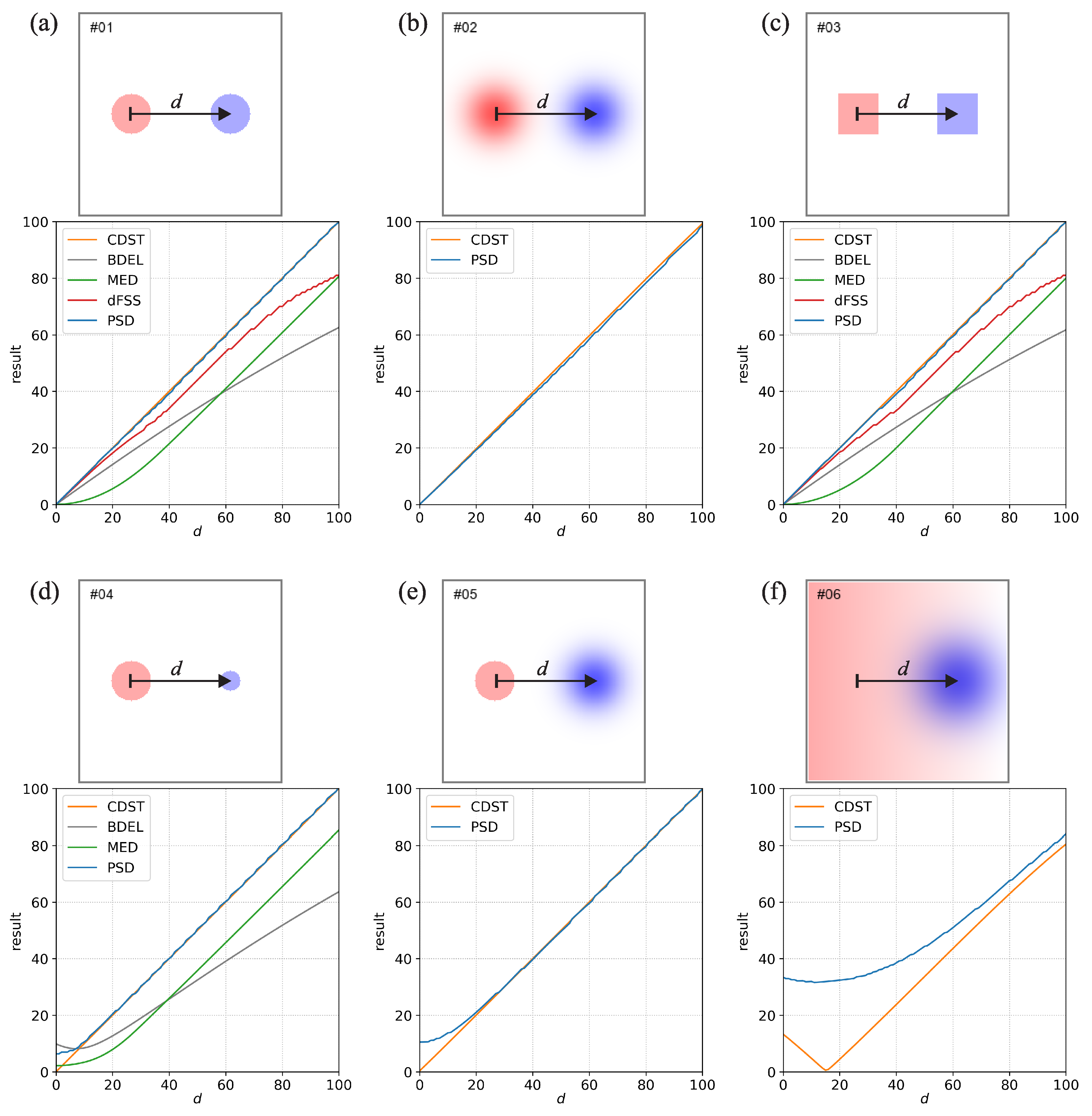
The behavior of the new method was analyzed by applying the new measure along with four other measures to a set of 23 situations with idealized geometric fields. The situations and the corresponding results are shown in Figure 1, Figure 2, Figure 3 and Figure 4. All comparisons are based on fields constructed on a 200 × 200 regular grid. Some of the situations are based on the cases from [3,12] while others are new. Some of the fields are binary, while others are multi-level or continuous. They are described in detail in the supplementary material. Each situation also depends on a variable parameter d, reflecting the displacement of one of the events. The results are always provided for a range of d values, starting from 0 and going to either 50 or 100 grid points. All the input fields that were used for the idealized situations are freely available on github (for details please refer to the Data Availability Statement at the end of the article).
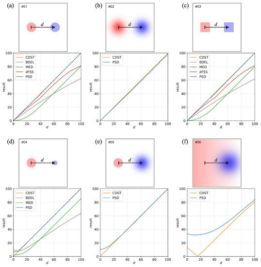
Figure 1.
The subfigures (a–f) show six idealized situations that were used to analyze the behavior of the distance measures. The top panel in each subfigure shows the layout of the idealized situation. The blue color corresponds to the values in the first field, and the red color corresponds to the values in the second field. The higher the value, the darker the respective color. The arrow marked with d shows the displacement of the event it is pointing to. For example, for , the blue circular event in (a) will completely overlap the red event, while for , the blue event is moved toward the right. The bottom panel in each subfigure shows the results of the distance metrics. Since the results depend on the d, they are provided for values ranging from 0 to 100 grid-points. If the value of a certain metric is undefined, its results are not shown (e.g., the input fields are non-binary, but the metric can only be used with binary fields).
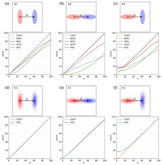
Figure 2.
Same as Figure 1 but for the six comparisons that use a pair of either binary or Gaussian events of elliptical shape.
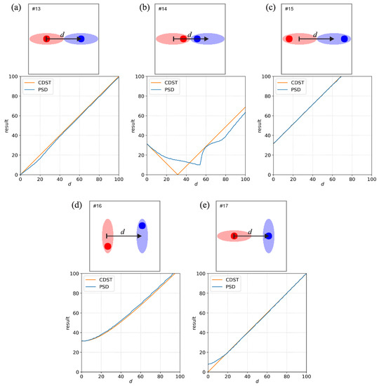
Figure 3.
Same as Figure 1 but for the six comparisons that use a set of displaced double-level events. The area with low-intensity values is elliptical but contains a smaller circular area with high-intensity values.
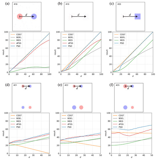
Figure 4.
Same as Figure 1 but for noisy, scattered and two-set event fields.
Figure 1 shows the first six comparisons denoted by indices #1 to #6. Comparisons #1–#3 (Figure 1a–c) use a single event of either circular, Gaussian, or square shape, with an identical but displaced event in the other field. The PSD and CDST give a near-perfect estimate of the actual displacement for the whole range of d values for the circular and square-shaped events. All other measures underestimate the displacement with the smallest underestimation provided by dFSS. For the Gaussian events, due to the events being non-binary, only PSD and CDST provide a result, with both giving a near-perfect estimate of the actual displacement for the whole range of d values.
For the dFSS, the underestimation is quite well documented and discussed in [3]. For example, Figure 3c in [3] shows that the relative underestimation is the largest when the displacement is equal to the diameter of the circular events. For comparisons #1–#3 the underestimation additionally increases for large displacements when d approaches 100. This happens due to the so-called border effect, which can result in dFSS underestimating the displacement if the events are located relatively close to the domain borders (this is also mentioned [3]). The border effect can be mitigated by increasing the domain size (this was not done here). Regarding MED, the likely cause of the underestimation is its reliance on distance maps generated via the nearest-neighbor methodology. When the MED between two non-overlapping events is calculated, the distance between the grid points of one event to the closest part of the second event is considered, which results in an underestimation. BDEL is also based on distance maps. Still, since the nearest-neighbor distances are evaluated over the whole domain, including the non-event regions, its behavior is more complicated and more difficult to interpret. For example, for comparison #1 at , reducing the domain size (thereby reducing the size of non-event regions that surround the central region with the two events) will decrease the BDEL value, while increasing the domain size will increase the value.
Comparison #4 (Figure 1d) is similar to #1 but uses circular events with different sizes (diameters 20 and 10 grid points). For , both PSD and CDST give a near-perfect estimate of the actual displacement, while the other measures underestimate it. Due to the two fields having a significant bias, the dFSS cannot provide a result. At , the CDST approaches zero as , while the decrease of PSD slows and is about 6 grid points at . The CDST being zero at is a consequence of the centers-of-mass of the two circular events being collocated. However, since the two fields are not identical, having a displacement of zero (which indicates a perfect forecast) does not make much sense. Since the overlap of the two events is not perfect, and parts of the larger event stick out from the area of the smaller event, it makes more sense that the displacement is larger than zero. Since the larger event sticks out from the smaller event for 0 to 10 grid points, with the middle being five grid points, the PSD result of 6 grid points seems quite reasonable.
Comparison #5 (Figure 1e) uses a circular and a displaced Gaussian event. Similarly to #2, only PSD and CDST provide a result, with both giving a near-perfect estimate of the actual displacement for . Similarly to Comparison #04, the CDST approaches zero as , while the decrease of PSD slows and is about ten grid points at .
Comparison #6 (Figure 1f) uses a linear gradient event, with values increasing from 0 to 1 from right to left, and a circular event. Again, since the gradient event is non-binary, only PSD and CDST provide results. Since the magnitude of the gradient event is the largest on the left side of the domain, the resulting estimates of displacements are largest when the circular event is on the right side (i.e., if d is large). At , both measures provide a similar result of grid points, but the difference between the two measures starts to increase when d decreases. At approximately , the PSD and CDST values are the smallest, with PSD being 31 grid points while CDST is zero. Again, CDST being zero does not make much sense since the two fields are, in fact, very different, regardless of the value of d.
Figure 2 shows the six comparisons that use a pair of either binary or Gaussian events of elliptical shape in various combinations of displacement and orientation. Comparisons #7 and #8 (Figure 2a,b) use a pair of identically oriented binary elliptically events. The PSD and CDST give a near-perfect estimate of the actual displacement for the whole range of d values. All other measures underestimate the displacement with the smallest underestimation provided by dFSS. The underestimation is especially large for #8 in the case of MED and BDEL, which is again linked to the nearest-neighbor methodology they are based on (due to the horizontal orientation, one end of the ellipse will always stick quite far out towards the center of the other ellipse). In comparison #9 (Figure 2c) the two elliptical events are perpendicular, with all the measures, except CDST, providing a larger than zero result for . At , the PSD and CDST give an excellent estimate of the actual displacement, while the other measures underestimate it. For the comparisons #10–#12 (Figure 2d–f), with the non-binary Gaussian elliptical events, only PSD and CDST can provide results, which are very similar to the ones for binary elliptical events (comparisons #7–#9).
Comparisons #13 to #17 (Figure 3) use a set of displaced double-level events in various combinations of displacement and orientation. The area with low-intensity values is elliptical but contains a smaller circular area with high-intensity values. Since the fields are non-binary, only the PSD and CDST provide results. The low and high-intensity regions’ magnitude (the sum of values) is comparable (the ratio is about 7.5:10). The positioning of the high-intensity regions is different for each comparison. In comparison #13 (Figure 3a), the centers of high and low-intensity areas are collocated, and both the PSD and CDST give a good estimate of the actual displacement. In contrast, in #14 and #15 (Figure 3b,c), the higher intensity areas are displaced either toward the center or to the sides. Depending on the overlap and distance between the low- and high-intensity regions, the resulting values can noticeably decrease or increase.
Since both fields in Comparison #14 are vertically symmetrical around the middle, the center of mass is located on the middle line. As d changes, the blue event is transposed in the left-right direction, and the distance between the centers of mass will change linearly—thus, the CDST will also change linearly with d. At approximately , the centers of mass of the two events are collocated, and . The behavior of PSD is roughly similar, with two local maximums at and 100 grid points and one minimum in the middle. The minimum of PSD is near when the two high-intensity regions have considerable overlap, while at the same time, there is also some overlap between the low-intensity regions.
Comparison #16 (Figure 3d) is similar to previous comparisons, but the ellipses are vertically aligned with the circular areas diagonally displaced. Comparison #17 (Figure 3e) is similar to #9 (Figure 2c), but the collocated higher intensity regions cause a slight reduction of the PSD value at small values of d.
It is worthwhile mentioning what would happen if comparisons #13 to #15 were analyzed using a metric that requires thresholding. If a single threshold value would be used that was smaller than the low-intensity precipitation denoted by the lighter colors, then comparisons #13 to #15 would all provide identical results. This happens since the binary fields for these three comparisons would be identical and all elliptical events inside the fields would be identical, regardless of the actually intensity of precipitation inside them. If the threshold would be set to an intermediate value (precipitation intensity that would correspond between the low- and high-intensities shown by lighter and darker colors), then the resulting binary events would represent only the small circular high-intensity regions while the low-intensity regions would be ignored. Of course, if the chosen threshold was higher than the high-intensity precipitation denoted by the darker colors, then there would be no events left after the thresholding. As PSD does not require thresholding it takes into account all the precipitation at the same time, while also taking note of the differences in its intensity.
Figure 4 shows the comparisons with noisy, scattered, and two-set event fields. Comparison #18 (Figure 4a) is the same as #1 (Figure 1a) but with a small amount of randomly generated noise in both fields. The results of the PSD, CDST, and dFSS for the noisy situation are almost the same as for the non-noisy situation, indicating that these metrics are not overly sensitive to noise. On the other hand, the noise greatly influences the MED and BDEL, with significantly smaller displacement estimates. This behavior indicates that the MED and BDEL are quite sensitive to small changes in the fields. The behaviour can be linked to the use of nearest-neighbor methodology they are based on. Namely, since the noisy events are more or less evenly spread out throughout the domain, it is never far to the nearest event, which results in a severely reduced estimate of the displacement. Moreover, BDEL has almost a constant value of about 11 grid points, which can be attributed to the nearest-neighbour distances being evaluated over the whole domain (which includes the regions without events).
Comparison #19 (Figure 4b) uses the so-called scattered events. Both fields contain small-scale single-grid-point events randomly scattered inside a square-shaped envelope. With respect to d, the two envelopes can be overlapping or are far apart. The real-world analogy is a region of small-scale convective systems, with the region being either correctly or incorrectly positioned in the forecast. For larger displacements, when the two envelopes do not overlap (e.g., grid points), the results are quite similar to comparison #3 (Figure 1c), which uses the fully-filled square-shaped events. However, when the two envelopes overlap, the results diverge from #3, with PSD and dFSS providing smaller displacement estimates. This behavior can be interpreted as measures transitioning from estimating the large-scale envelopes’ displacement toward the displacement of individual small-scale events in the overlapping portions of the envelopes. At , the envelopes overlap fully, and all metrics provide an estimate between 2 and 3 grid points, which corresponds quite well to the average nearest-neighbor distance between the single-grid-point events. Even CDST is not zero at , which might be surprising since the centers of the two envelopes are collocated. The reason is that the small-scale events in the two envelopes are randomly generated, resulting in the centers of mass of the two fields not necessarily being collocated.
Comparison #20 (Figure 4c) is a mix of comparisons #3 and #19. One field contains the square-shaped envelope with small-scale scattered events, while the other contains a fully-filled square-shaped event of identical size. While the dFSS cannot provide a result (due to the bias being too large), the results of other methods are similar to comparison #19. However, there are some differences at smaller values of d when the two square-shaped regions overlap. For example, at , PSD is 2.7, CDST 0.3, BDEL 4.5 and MED is 1.5 grid points.
Comparisons #21 to #23 (Figure 4d–f) use two sets of events. The sets are located near the top or the bottom of the domain. The d reflects the displacement of the events in the top set only, while the displacement in the bottom set is fixed to 50 grid points. These setups are interesting as they indicate how the metrics behave in a multi-event situation.
In #21 (Figure 4d) all the events are identical. At most of the metrics provide results of about 25 grid points (except MED, which is about 20 grid points). A displacement of approximately 25 grid points makes sense since this is the average displacement of the events in the two sets—at , the displacement of the top set is zero, and the displacement of the bottom set is always 50 grid points. As d increases, so do the values of all measures (except CDST). PSD and dFSS increase more or less linearly with d and are close to 50 grid points at —thus, they both approximate well the average displacement of the events in the two sets. The values of BDEL and MED tend to be somewhat smaller and behave less linearly with respect to d. Contrary to other measures, CDST decreases with d and reaches 0 at . This is again linked to the centers of mass of the two fields being collocated. Namely, since all the events are identical, the center of mass of each field will always be located on the middle line between the bottom and top domain borders. At , the centers of mass of both fields are collocated in the exact center of the domain, resulting in CDST = 0.
Comparison #22 (Figure 4e) is similar to #21, but the events in the bottom set are larger (the magnitude of events in the bottom set is twice the magnitude of the events in the top set). A real world analogy would be a two pairs of stronger and weaker precipitation events. At the PSD, dFSS and CDST are close to 33 grid points, which is the magnitude weighted average displacement of the events in the two sets (i.e., ). As d increases, the PSD and dFSS also increase more or less linearly to about 50 grid points at —thus, they approximate well the magnitude weighted average displacement of the events in the two sets. On the other hand, the CDST again decreases with d, and the BDEL and MED values tend to be smaller than PSD and dFSS. Surprisingly, the BDEL values are almost identical to #21, which indicates that the magnitude of events does not influence the results. This behavior can likely be attributed to the nearest-neighbor distances being evaluated over the whole domain instead of only the areas with events. The larger size of the events probably does not significantly affect the distance maps in most parts of the domain, and the BDEL value remains almost the same.
In comparison #23 (Figure 4f), the events in each set are biased—there is a larger and a smaller event in each set. Again BDEL values are almost identical to #21 for the same reasons as for #22. Surprisingly, MED values are also practically identical to #21. This behavior can be attributed to the nearest-neighbor methodology used by MED. Only the distance to the nearest event is evaluated, regardless of how big or small that event might be. On the other hand, PSD, dFSS, and CDST are markedly larger compared to #21. This behavior makes sense—since each set is biased, one could expect the displacement to be larger since the events of each set do not balance each other out perfectly. The behavior of CDST is nearly linear with respect to d, but its value does not change much. The center of mass of one field is located more towards the top, while the center of mass of the other field is more towards the bottom. The vertical distance between the centers of mass is larger than the horizontal (which depends on d) so the CDST does not change much with d. The behavior of PSD and dFSS is more variable and complex, with PSD consistently larger compared to dFSS. They both have a global minimum at approximately grid points and are larger for other values of d.
Figure 5 shows the results of six additional non-spatial measures for comparison #1 with the displaced circular events. Figure 5 can be compared with the bottom panel of Figure 1a, which shows the results of the distance metrics. The non-spatial measures are the root-mean-square-error (RMSE, [13]) and five measures based on contingency tables: the probability of detection (POD, also called hit rate), false alarm ratio (FAR), critical success index (CSI, also called threat score), Heidke skill score (HSS) and Gilbert skill score (GSS, also called equitable threat score). The description of the five contingency-table-based measures is available in [14].
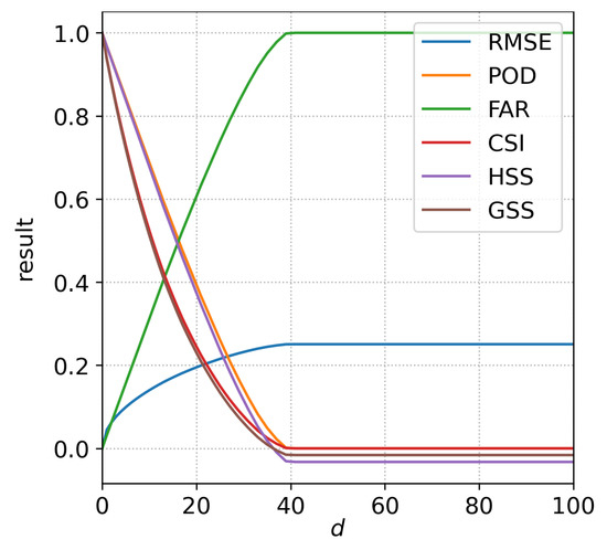
Figure 5.
Same as the bottom frame of Figure 1a but instead of the distance metrics, the results of six non-spatial measures are shown: root-mean-square-error (RMSE), probability of detection (POD, also called hit rate), false alarm ratio (FAR), critical success index (CSI, also called threat score), Heidke skill score (HSS) and Gilbert skill score (GSS, also called equitable threat score).
If the forecast is perfect (i.e., ) the values of the non-spatial measures are either 0 (RMSE, FAR) or 1 (POD, CSI, HSS, GSS). As d increases, the overlap becomes smaller, and the values of RMSE and FAR increase, while the values of other measures decrease, which is as expected. However, once d reaches 40, their values do not change anymore (for example, FAR starts at 0 and increases towards the worst possible value of 1 at , but does not change when the displacement is further increased). This happens since the overlap becomes zero at and remains zero for all larger values of d. Thus, as long as there is no overlap, the non-spatial measures will always give identical results regardless of the actual displacement. Clearly, this behavior does not make much sense since the forecast is evidently better if instead of . All non-spatial methods will display such behavior since they only compare values at collocated grid points. The distance metrics, which are spatial methods, do not exhibit such behavior (Figure 1a). They clearly show that the forecast error grows even after d is larger than 40, with the best estimates of actual displacement provided by PSD and CDST. It is also worth noting that large displacements of precipitation are common in real-world situations. For example, in a 9-day forecast, large-scale phenomena like cyclones will frequently be positioned at completely wrong locations. Since most precipitation in the mid-latitudes can be attributed to the frontal systems located inside the cyclones, the displacement will be large, and the likelihood of precipitation in the forecast not overlapping with the actual precipitation will be high.
Also, when , the value of RMSE will decrease if the forecast field is set to zero (not shown) – meaning that it would be better in terms of score’s value for the model to predict no precipitation as opposed to predicting at least some precipitation at some non-overlapping location. This is an example of the so-called ’double penalty problem’ mentioned in the introduction, where a forecast is penalized for predicting an event where it did not occur and again for failing to predict the event where it occurred. The HSS and GSS also exhibit such behavior, although the impact on their values is relatively small (not shown).
3.2. Analysis of Real-World Examples
While the analysis of idealized examples provides numerous valuable insights into the properties of the new metric, it is also important to demonstrate its behavior in real-world examples. Figure 6 shows some examples of 6-hourly precipitation forecasts over Europe and North Africa (domain size grid points and resolution). The examples are taken from the study done by Skok and Roberts [15]. The forecasts were calculated by the European Centre for Medium-range Weather Forecasting (ECMWF) model, with 6-hourly analysis precipitation (0000-0600 UTC precipitation accumulations) compared with the corresponding precipitation from the 1-, 5- and 9-day forecast. We only studied the PSD since we wanted to analyze the full continuous fields and did not want to use thresholding (the MED and BDEL can only provide results for binary input fields). While the CDST can be used with non-binary fields, we nevertheless decided not to use it here since the analysis of idealized cases showed that it often does not provide meaningful results.
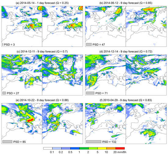
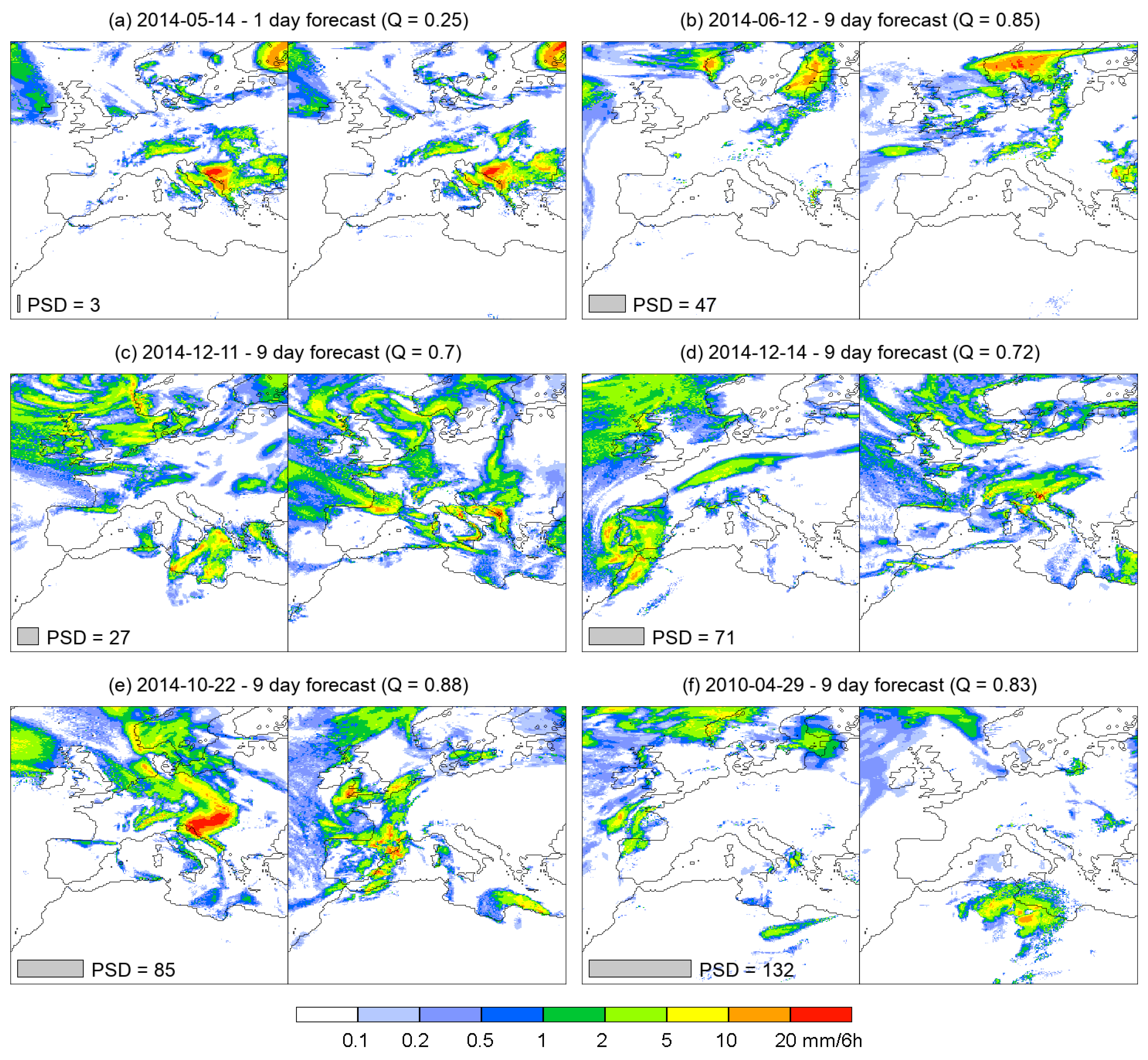
Figure 6.
PSD for selected examples of 6-hourly operational ECMWF precipitation forecasts over Europe and North Africa. The domain size is grid points. The left panel of each figure shows the analysis precipitation, while the right panel shows the forecast for the same 6-h period. The gray bar in the lower-left corner represents the estimate of displacement provided by PSD. The value of the Q parameter is also provided in each panel title.
Figure 6a shows a 1-day forecast, which is very similar to the analysis. The majority of precipitation is overlapping (Q = 0.25). Thus, the resulting PSD value is small (3 grid points). Figure 6b shows a 9-day forecast with most of the precipitation concentrated in either one or two dominating events. The single dominating event in the forecast is located between the two events in the analysis. There is very little overlapping precipitation (Q=0.85), which results in a medium PSD value of 47 grid points.
Figure 6c,d show situations with multiple events spread out over a large portion of the domain. In both cases, about 30% of precipitation is overlapping. At the same time, the regions of precipitation in Figure 6c are less displaced, resulting in a lower PSD value (27 grid points), compared to Figure 6c, where the PSD value is larger (71 grid points).
Figure 6e,f show 9-day forecasts that are very different from the analysis. There is less than 20% of overlapping precipitation, and the displacement is large. In Figure 6e, most of the precipitation in the forecast can be found over Western Europe, with the largest amount of precipitation in the analysis located over the western Balkans, which results in a rather large PSD value of 85 grid points. The displacement is even larger in Figure 6f, with most precipitation located either in the NW part of the domain or over North Africa, resulting in an even larger PSD value of 132 points.
Finally, Figure 7 shows the analysis of time-series of ECMWF precipitation forecasts for the same domain as before. It shows the monthly and yearly averages of PSD values for the 6-h precipitation accumulations (0000–0600 UTC) in the period 2007-2014. There is a clear difference between the 1-, 5-, and 9-day forecasts, with the average PSD values being approximately 5, 25, and 49 grid points, respectively. The corresponding values of standard deviations of PSD are 2, 13, and 24 grid points. The relatively large standard deviations indicate a large spread of the PSD values that presumably reflect various weather situations that can be present in the analyzed domain. Nevertheless, the series of yearly averages of PSD values has a statistically significant decreasing trend for the 1-day forecast ( grid points/year, significant at ) and the 5-day forecast ( grid points/year, ). The 9-day forecast does not have a significant trend. A modified Mann-Kendall test that utilizes a trend-free pre-whitening method [16] was used to determine the statistical significance of a trend. The decreasing and significant trends of the 1- and 5-day forecasts show a clear improvement in the forecasting ability of the ECMWF model, with regards to spatial displacement of precipitation, despite the analyzed period of 8 years being rather short. The 1- and 5-day forecasts also exhibit a noticeable seasonal dependence of PSD values, with the forecast being better during the cold part of the year. The seasonal variation of the PSD value is likely linked to the frequency of occurrence of convective precipitation (which is more challenging for the model to predict since convection is a sub-grid process), which appears more frequently in the warmer part of the year.
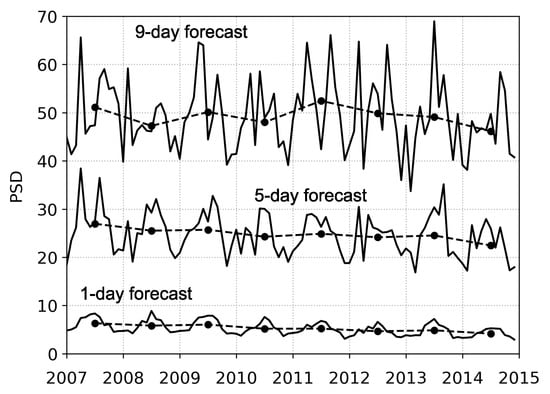
Figure 7.
Analysis of time-series of ECMWF precipitation forecasts. Monthly (solid line) and yearly (dash-dotted line with circles) averages of PSD values for the 6-h precipitation accumulations (0000–0600 UTC) in the period 2007–2014.
In order to determine if the ECMWF forecast possesses some minimal measure of skillfulness, its PSD values can be compared to the PSD values of the corresponding persistence forecasts. The persistence forecast assumes that the future state of the atmosphere (in this case, the precipitation that falls in 6 hours) is assumed to be identical to the current state of the atmosphere (the analysis precipitation). In the meteorological community, the persistence forecast is frequently used as a benchmark for evaluating forecast skill. As long as the error of the model’s forecast is smaller than the error of the persistence forecast, the model could be considered to possess some minimal measure of skillfulness, whereas if the reverse is true, the model can be considered to possess no skill. Current state-of-the-art NWP prediction models tend to beat the persistence forecast by a large margin at short lead times. However, at longer lead times (e.g., 10-days or more), the model’s error can become comparable to or larger than the error of the persistence forecast. In our case, the mean PSD values for the corresponding 1-, 5-, and 9-day persistence forecasts are 40, 59, and 61 grid points. As expected, for the 1-day forecast, the ECMWF model is much better than the persistence forecasts, with PSD being approximately ten times smaller for the ECMWF model. For the 5-day forecast, the ECMWF model is still significantly better, with the model’s PSD being about half of the PSD of the persistence forecast. For the 9-day forecast, the ECMWF model is still superior, but the difference is smaller since the model’s PSD is only about 20% smaller than the persistence forecast’s. This indicates that the model possesses only a limited amount of skill when used to perform the 9-day forecasts.
4. Discussion and Conclusions
In this study, a new spatial distance metric for precipitation is presented. The new metric is meant to be used by meteorologists and atmospheric scientists who want to compare or evaluate the predictive skill of multiple numerical weather prediction models or determine if a newer version of the same model has a better predictive skill than the older version. In order to determine if the model possesses some minimal measure of skillfulness, the metric can also be evaluated for the model’s forecasts and the corresponding persistence forecasts, and the results compared.
Contrary to most other distance metrics, the PSD does not require thresholding (although it can still be used if one wishes to) and can thus be used to analyze binary and non-binary (e.g., continuous or multi-level) fields. Similar to other distance measures, it provides a global estimate of spatial distance, a single value related to the spatial distribution of all events present in the two fields (as opposed to providing a different value for each individual event).
The analysis of 23 comparisons with idealized geometric fields showed that the new metric provides a good and meaningful approximation of the displacement in situations with a single displaced event. Typically the estimate of displacement provided by PSD was better than the results provided by most other metrics. For situations with multiple events, the measure’s behavior was not inconsistent with a subjective evaluation. The analysis also showed that the measure is not overly sensitive to noise, its results are directly related to the actual displacements of events, and that the events with a larger magnitude have a bigger influence on the resulting value.
The analysis of ECMWF precipitation forecasts over Europe and North Africa confirmed that the new metric provides a meaningful approximation of the displacement in real-world situations. If a sequence of fields is analyzed, the uncertainty of the mean PSD value can be estimated via statistical parameters linked to the width of the distribution (e.g., standard deviation, 10 and 90 percentile). The trend and its statistical significance can be determined using an appropriate variant of the Mann-Kendall test, which properly accounts for the autocorrelation present in the time series.
The value of the new metric can be calculated efficiently via the use of Fast-Fourier-Transform-based convolution and the Bisection method. A python code package for efficient calculation of the PSD value is freely available.
In the end, it is important to acknowledge that spatial displacement is only one type of forecast error [3]. It is thus always necessary to simultaneously use multiple metrics that can analyze different aspects of forecast performance. One example is the bias, which is a useful complementary measure to the PSD since it ignores the differences in the spatial distribution of precipitation and only compares the precipitation sums in the two fields.
Supplementary Materials
The following supporting information can be downloaded at: https://www.mdpi.com/article/10.3390/app12084048/s1, Section S1 includes a detailed description of how the new metric was devised, Section S2 provides a description of the comparisons with idealized geometric fields. Ref. [17] is cited in supplementary material.
Author Contributions
Conceptualization, G.S.; methodology, G.S.; software, G.S.; validation, G.S.; formal analysis, G.S.; investigation, G.S.; resources, G.S.; data curation, G.S.; writing—original draft preparation, G.S.; writing—review and editing, G.S.; visualization, G.S.; supervision, G.S.; project administration, G.S.; funding acquisition, G.S. All authors have read and agreed to the published version of the manuscript.
Funding
The authors acknowledge the financial support from the Slovenian Research Agency (Javna Agencija za Raziskovalno Dejavnost RS; research core funding No. P1-0188 and project J1-9431).
Data Availability Statement
A python code package for efficient calculation of the PSD value is freely available on https://github.com/skokg/PSD (DOI:10.5281/zenodo.6334211) (accessed on 14 April 2022). The input fields that were used for the idealized situations are freely available at netcdf fields on https://github.com/skokg/PSD_idealized_netcdf_fields (DOI:10.5281/zenodo.6334220) (accessed on 14 April 2022). The code and the idealized input fields can also be obtained upon request from the corresponding author.
Conflicts of Interest
The authors declare no conflict of interest. The funders had no role in the design of the study; in the collection, analyses, or interpretation of data; in the writing of the manuscript, or in the decision to publish the results.
References
- Brown, B.G.; Gilleland, E.; Ebert, E.E. Forecasts of Spatial Fields. In Forecast Verification; John Wiley and Sons, Ltd.: Chichester, UK, 2012; pp. 95–117. [Google Scholar] [CrossRef]
- Dorninger, M.; Gilleland, E.; Casati, B.; Mittermaier, M.P.; Ebert, E.E.; Brown, B.G.; Wilson, L.J. The setup of the MesoVICT project. Bull. Am. Meteorol. Soc. 2018, 99, 1887–1906. [Google Scholar] [CrossRef]
- Skok, G.; Roberts, N. Estimating the displacement in precipitation forecasts using the Fractions Skill Score. Q. J. R. Meteorol. Soc. 2018, 144, 414–425. [Google Scholar] [CrossRef]
- Davis, C.A.; Brown, B.G.; Bullock, R.; Halley-Gotway, J. The Method for Object-Based Diagnostic Evaluation (MODE) Applied to Numerical Forecasts from the 2005 NSSL/SPC Spring Program. Weather. Forecast. 2009, 24, 1252–1267. [Google Scholar] [CrossRef] [Green Version]
- Baddeley, A.J. An error metric for binary images. In Robust Computer Vision; Förstner, W., Ruwiedel, S., Eds.; Wichmann: Karlsruhe, Germany, 1992; pp. 59–78. [Google Scholar]
- Gilleland, E. A new characterization within the spatial verification framework for false alarms, misses, and overall patterns. Weather. Forecast. 2017, 32, 187–198. [Google Scholar] [CrossRef]
- Roberts, N.M.; Lean, H.W. Scale-Selective Verification of Rainfall Accumulations from High-Resolution Forecasts of Convective Events. Mon. Weather. Rev. 2008, 136, 78–97. [Google Scholar] [CrossRef]
- Roberts, N. Assessing the spatial and temporal variation in the skill of precipitation forecasts from an NWP model. Meteorol. Appl. 2008, 15, 163–169. [Google Scholar] [CrossRef] [Green Version]
- Mittermaier, M.; Roberts, N.; Thompson, S.A. A long-term assessment of precipitation forecast skill using the Fractions Skill Score. Meteorol. Appl. 2013, 20, 176–186. [Google Scholar] [CrossRef]
- Press, W.H.; Teukolsky, S.A.; Vetterling, W.T.; Flannery, B.P. Numerical Recipes 3rd Edition: The Art of Scientific Computing, 3 ed.; Cambridge University Press: Cambridge, MA, USA, 2007. [Google Scholar]
- Smith, S.W. The Scientist and Engineer’s Guide to Digital Signal Processing; California Technical Publishing: San Diego, CA, USA, 1999. [Google Scholar]
- Gilleland, E.; Skok, G.; Brown, B.G.; Casati, B.; Dorninger, M.; Mittermaier, M.P.; Roberts, N.; Wilson, L.J. A Novel Set of Geometric Verification Test Fields with Application to Distance Measures. Mon. Weather. Rev. 2020, 148, 1653–1673. [Google Scholar] [CrossRef]
- Déqué, M. Deterministic Forecasts of Continuous Variables. In Forecast Verification; Wiley: New York, NY, USA, 2011; pp. 77–94. [Google Scholar] [CrossRef]
- Manzato, A.; Jolliffe, I. Behaviour of verification measures for deterministic binary forecasts with respect to random changes and thresholding. Q. J. R. Meteorol. Soc. 2017, 143, 1903–1915. [Google Scholar] [CrossRef]
- Skok, G.; Roberts, N. Analysis of Fractions Skill Score properties for random precipitation fields and ECMWF forecasts. Q. J. R. Meteorol. Soc. 2016, 142, 2599–2610. [Google Scholar] [CrossRef]
- Yue, S.; Wang, C.Y. Applicability of prewhitening to eliminate the influence of serial correlation on the Mann-Kendall test. Water Resour. Res. 2002, 38, 4-1–4-7. [Google Scholar] [CrossRef]
- Weisstein, E.W.; Circular Segment. From MathWorld—A Wolfram Web Resource. Available online: https://mathworld.wolfram.com/CircularSegment.html (accessed on 7 January 2022).

Publisher’s Note: MDPI stays neutral with regard to jurisdictional claims in published maps and institutional affiliations. |
© 2022 by the author. Licensee MDPI, Basel, Switzerland. This article is an open access article distributed under the terms and conditions of the Creative Commons Attribution (CC BY) license (https://creativecommons.org/licenses/by/4.0/).