Abstract
Assessment of a corroded pipe is crucial to determine when it must be repaired or replaced. However, the conventional corrosion assessment codes for the failure pressure predictions of corroded pipes with circumferentially aligned interacting defects are conservative (underestimations of more than 40%), resulting in premature repair or replacements of pipelines. Alternatively, numerical approaches may be used, but they are time consuming and computationally expensive. In this study, an analytical equation based on finite element analysis for the failure pressure prediction of API 5L X52, X65, and X80 corroded pipes with circumferentially aligned interacting corrosion defects subjected to combined loadings is proposed. An artificial neural network trained with failure pressure obtained from the finite element analysis of the three pipe grades for varied defect spacings, depths and lengths, and axial compressive stress were used to develop the equation. Subsequently, a parametric study on the effects of these parameters on the failure pressure of a corroded pipe with circumferential-interacting defects was conducted using the equation to determine the correlation between the defect geometries and failure pressure of the pipe. The new equations predicted failure pressures for these pipe grades with an R2 value of 0.99 and an error range of −9.92% to 0.98% for normalised defect spacings of 0.00 to 3.00, normalised effective defect lengths of 0.00 to 2.95, normalised effective defect depths of 0.00 to 0.80, and normalised axial compressive stress of 0.00 to 0.60.
1. Introduction
Over the past decades, researchers have investigated and established the severity of damage caused by corrosion defects in API 5L X52, X65, and X80 oil and gas pipelines, which are commonly used in the industry [1,2,3,4,5,6,7,8,9,10,11]. Generally, corrosion can be divided into three categories, which are single defects, interacting defects, and complex defects [12]. Single defects are corrosion defects that have no interaction with neighboring defects. They are sufficiently isolated from the surrounding defects, resulting in no overlapping regions of stress and strain disturbance. Unlike single defects, the overlapping regions of stress and strain disturbance are present for interacting defects [4,7]. For two defects that are in close proximity (within the interaction limit), the stress concentration is the highest at the overlap region. As such, the threat imposed by interacting defects is much more severe than that of single defects. As for complex defects, it is another form of interacting defects, where a cluster of defects is present. Table 1 illustrates the difference between single, interacting, and complex defects. Each type of defect orientation exhibits different failure pressure behavior. This study focuses on circumferentially aligned interacting corrosion defects.

Table 1.
Classification of defects [12].
1.1. Conventional Corrosion Assessment Codes
Various corrosion assessment methods have been developed to assess the integrity of a pipeline under various conditions to ensure safe operations. Failure pressure predictions based on conventional corrosion assessment codes, such as ASME B31G, Modified B31G, SHELL 92, RSTRENG, PCORRC, and DNV-RP-F101, are conservative, resulting in premature pipeline repairs and replacements [13]. Of all the codes that are being used in the industry for failure pressure prediction of corroded pipes subjected to combined loading, the DNV-RP-F101 code (DNV) is the most comprehensive [2,6,14,15,16,17].
Over the years, various studies have been carried out to develop accurate interaction rules based on corrosion defect categories such as longitudinal interacting defects, circumferential interacting defects, or single defects. The interaction rule applied for circumferentially aligned interacting defects in commonly used corrosion assessment codes in the industry are presented in Table 2.
Table 2.
Interaction rules applied for circumferentially aligned interacting defects in common corrosion assessment methods [18].
However, since the validation of the DNV approach was based on burst tests carried out on pipes of grades API 5L X45 to API 5L X65, it was designed primarily to examine the integrity of medium toughness pipelines. When applied to high toughness pipelines, it results in inaccurate and overly conservative predictions [4,6]. In addition, this method is only applicable for interacting defects subjected to internal pressure only.
1.2. Artificial Neural Network as a Failure Pressure Prediction Tool
The utilization of an artificial neural network (ANN) in the field of failure pressure assessment has improved over the years, resulting in more practical applications. In early applications of ANN, researchers took into account the physical, mechanical, operational, and environmental factors that influenced the residual strength of a pipeline [19].
Liu et al. [20] developed a multilayer feedforward neural network with backpropagation learning algorithms for predicting the failure pressure of X80 pipe with corrosion defects caused by stray current. By comparing the ANN model results to experimental burst test results and earlier failure pressure estimate model findings, it was established that the ANN model results are both accurate and efficient with a R2 value of 0.9992. Zangenehmadar et al. [19] also used this approach in their research to determine the useful life of pipelines using the Levenberg–Marquart backpropagation algorithm. Their ANN model was able to predict the useful life of a pipeline with an error percentage of less than 5%.
The architecture of an ANN is determined by the data type and desired output. The feedforward neural network algorithm is primarily used to predict the failure pressure of corroded pipelines. This form of ANN architecture (Figure 1) is designed to learn from paired datasets, in which the model is trained using one or more inputs and the matching output of the training dataset. A feedforward neural network is simple to implement and is well-suited for delivering a single output. Generally, a feedforward neural network is used with the Levenberg–Marquardt backpropagation approach to train the model, as it performs well and requires less time and epochs for convergence [21].
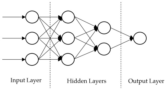
Figure 1.
A feedforward neural network with two hidden layers.
For ANN applications, a small dataset is not recommended as it will not generalise the data well. Shirzad et al. [22] and Senouci et al. [23] emphasised in their paper that an ANN model with reasonable accuracy and robustness cannot be achieved without sufficient real-life data. In such models, a comprehensive input is needed to ensure that the model is accurate. Hence, large training datasets need to be gathered [23]. However, obtaining a large training dataset for such cases is challenging.
1.3. Finite Element Method as a Failure Pressure Prediction and Data Generation Tool of Corroded Pipes
In this approach, the issue of having a limited amount of real-life data to generate training data for the ANN model can be overcome by using a Finite Element Method (FEM). FEM has been widely applied in the industry and among researchers for predicting the failure pressure or residual strength of a corroded pipeline. Using FEM, Lee et al. in 2005 assessed the failure of an API 5L X65 gas pipe at multiple corrosion defect regions with a maximum percentage error of less than 10.00% [5]. Similarly, Belachew et al. [8] utilised FEM for burst test analysis of a corroded API 5L X52 grade steel pipe with a maximum percentage error of less than 5.00%. The results of this study also showed that FEM is a reliable tool to analyse the effects of defect geometries on the failure pressure of the pipe.
In a study conducted by Xu et al. [24], an ANN was developed for the failure pressure prediction of a pipe with interacting corrosion defects using FEM to generate training data for ANN. A feed forward neural network was utilised with a backpropagation algorithm. Their ANN was developed with four neurons in the input layer, five neurons in the hidden layer, and one neuron in the output layer. The input parameters are the normalised defect length, depth, longitudinal spacing, and circumferential spacing. The number of neurons in the hidden layer was calculated using Equation (1), where is the number of hidden neurons, is the number of inputs while is the number of outputs. The developed ANN was validated against burst tests, and it was revealed that ANN can predict the failure pressure of a corroded pipe to a high level of accuracy, with a maximum percentage difference of 2.00%.
1.4. Development of Empirical Equations for Corroded Pipe Failure Pressure Prediction
Tohidi and Sharifi [25] developed an empirical equation for the prediction of the load-carrying capacity of locally corroded steel-plate girder ends based on an artificial neural network. Lo et al. [4] applied this approach in an effort of developing an empirical equation for the failure pressure of medium toughness corroded pipelines with longitudinal interacting corrosion defects subjected to combined loadings. Based on their study, it was found that the development of an empirical equation using the weights and biases of an ANN shows promising results. The developed equations predicted the failure pressure of a corroded API 5L X65 with longitudinal interacting corrosion defects with a maximum percentage difference of 2.26%.
While there are a few research studies [26,27,28,29] on the effects of internal pressure and axial compressive stress on the failure pressure of a high toughness pipe with circumferentially aligned interacting corrosion defects, there are no analytical closed form solutions for the failure pressure prediction of high toughness corroded pipeline subjected to internal pressure and axial compressive stress. Despite being the most comprehensive failure pressure assessment method in the industry, the DNV code incorporates internal pressure and axial compressive stress for the assessment of single defects only. As for interacting defects, it considers internal pressure only.
Furthermore, the DNV method was primarily developed to assess the integrity of low to medium toughness pipelines, as the validation of this method was based on full-scale burst tests conducted on pipes of grades API 5L X45 to API 5L X65 [12]. Hence, this method results in inaccurate failure pressure predictions when applied for high toughness pipes [6]. For these reasons, a DNV-like assessment method that incorporates combined loadings for the failure pressure prediction of high toughness pipelines with circumferentially aligned interacting corrosion defects is necessary. In addition, with empirical equations, failure pressure predictions can be obtained instantly, which is an important feature in time critical situations. Hence, an accurate and fast failure pressure assessment method is necessary for practical applications and the analysis of the failure pressure prediction of corroded high-toughness pipelines.
In this study, an empirical equation for the failure pressure prediction of the commonly used API 5L X52, X65, and X80 pipes with circumferentially aligned interacting corrosion defects subjected to internal pressure and axial compressive stress was developed using the weights and biases of an ANN model that was trained using data generated using FEM.
2. Materials and Methods
This study is based on quantitative data analysis where primary data are generated using computer-aided simulations using ANSYS 16.1 Structural Product of Mechanical ANSYS Parametric Design Language (APDL) for the failure pressure prediction of circumferentially aligned interacting corrosion defects subjected to combined loading. During the data preparation phase, failure pressure datasets were gathered by generating the training data using FEM. This was followed by data assessment and validation to ensure that there were no faulty data; outliers are removed; and the data conforms to a standardised pattern. Upon obtaining an organised failure pressure database, the data were transformed to reach a well-defined outcome using ANN. The first step in the development of the artificial neural network was to generate comprehensive training data for circumferentially aligned interacting corrosion defects subjected to internal pressure and axial compressive stress for pipe grades ranging from medium to high toughness materials. The second step involves the development and training of the ANN, followed by the development of the empirical equation.
2.1. Generation of ANN Training Data
2.1.1. Overview of Geometric Parameters for Generation of ANN Training Data
The training data for the ANN was generated using finite element analysis (FEA) for a range of parameters for API 5L X52, X65, and X80 pipe grades. The material properties are tabulated in Table 3, and the geometric parameters of the corroded pipe is tabulated in Table 4. The material properties of the pipe body are represented by a nonlinear true stress–strain curve of the materials during finite element simulations, as illustrated in Figure 2. FEM has proven to be a reliable tool for structural analysis and many researchers have utilised this method to generate training data for the development of ANN [4,25]. However, prior to FEA, FEM was validated against full-scale burst tests to ensure that the methodology and applied boundary conditions are correct. The results of the finite element analysis used as the training data for the developed ANN can be found in Supplementary Materials. A total of 1353 datasets were generated.
Table 3.
Material properties of the pipe grades used in this study.
Table 4.
Geometric parameters of the corroded pipe models.
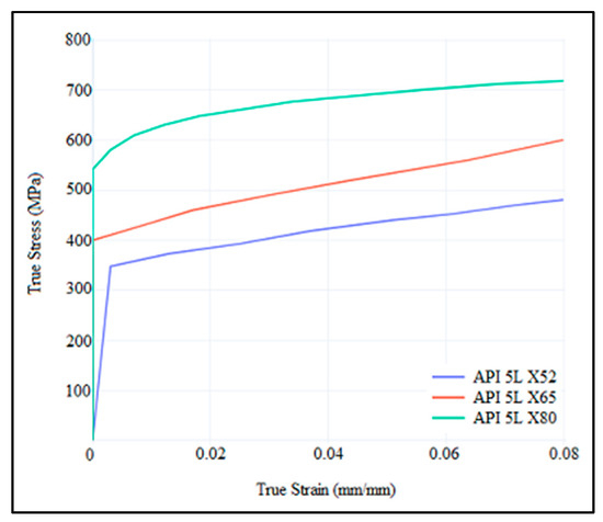
Figure 2.
True stress–strain curves for API 5L X52 [2], X65 [3], and X80 steel pipes [18].
2.1.2. Modelling and Meshing of the Quarter Models
In this study, quarter pipes with a rectangular shape idealization of corrosion defects were modelled using AutoCAD. Quarter models reduce computation time, while rectangular defect idealization allows for a safer, lower bound failure pressure prediction without compromising accuracy. The pipes were modelled with end caps for even distributions of axial compressive stress, and the full length of the model was set to 2000 mm to eliminate end-cap influence [2,4,8,12]. Figure 3 illustrates an example of the quarter model used during FEA.
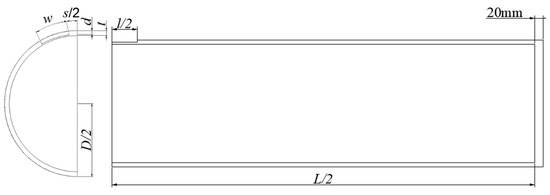
Figure 3.
Quarter pipe model of a pipe with circumferentially aligned interacting corrosion defects.
Prior to finite element simulations, the quarter models were meshed using ANSYS 16.1 Structural Product of Mechanical ANSYS Parametric Design Language (APDL), referred to as ANSYS. Hexahedral SOLID185 (linear order) and tetrahedral SOLID186 (quadratic order) elements were used to mesh the pipe body and end cap, respectively [2,4,8,30,31]. These elements were used to represent the solid structure, while shell elements were used to represent the outer surface of a structure [32].
With a total of three layers and mesh size of 2 mm in length and depth, the mesh settings at the defect region are in line with the recommendations by the British Standards Institution (BSI) [33]. Prior to finalizing the mesh settings, a convergence test was carried out to optimise the number of elements to ensure minimum computation time without compromising accuracy. Moving away from the defect region, a mesh bias with an aspect ratio of 0.5 was applied to the elements with a total of 80 divisions. The details and results of the convergence test are presented in Table 5.
Table 5.
Convergence test details and results.
2.1.3. Application of Boundary Condition
Since quarter models were utilised in this study, symmetrical boundary conditions were applied to the model for the model to be treated as an entire pipe. The degrees of freedom (DOF) in the x, y, and z directions were constrained at 4/5 of the model length away from the region of interest. As for the applied loadings in this transient analysis, incremental ramped loading was used to apply internal pressure and axial compressive stress on the pipe walls [2,8]. The loadings were applied in two timesteps: First, axial compressive stress was applied, then internal pressure was applied during the second timestep. The following assumptions were made during FEA:
- Isothermal condition (constant temperature throughout the simulation);
- Isotropic and homogenous pipe model (uniform material properties in all directions).
2.1.4. Failure Criterion
The failure pressure was determined using von Mises stress-based criterion, where the pipe is said to have failed when the von Mises stress reaches the true ultimate tensile strength of the material [2,34,35]. As the defect region is the most critical part of the pipe, the von Mises stress is concentrated at this region and ultimately causes the pipe to fail when the stress penetrates throughout the wall’s thickness. In ANSYS, the von Mises stress is calculated as a function of hoop, radial, and axial stress. The failure pressure of the pipe is the effective stress when it equals the true ultimate tensile strength of the material used.
2.1.5. Validation of the Finite Element Method
Before proceeding with FEA, FEM was validated against burst tests to ensure its accuracy and correct application of loads. Burst tests carried out by Bjorney et al. [36] and Benjamin et al. [37] were used to validate the method. The summary and results of the validation is presented in Table 6 and Table 7. The greatest difference between the results obtained from FEM and burst tests was only 5.92% and 2.46% for single and interacting defects respectively. Negative values indicate conservative predictions, with the predicted pressure not exceeding the actual failure pressure. Hence, it is evident that FEM is reliable in order to be used as a failure pressure data generation tool for the training of ANN.
Table 6.
Summary of burst test details by Bjorney et al. and Benjamin et al.
Table 7.
FEM validation against full scale burst tests by Bjorney et al. and Benjamin et al.
2.2. Development and Training of the Artificial Neural Network
The optimization of the neural network in terms of the number of hidden layers and neurons was based on a convergence test. The aim was to develop a neural network with the least number of neurons, as the complexity of the empirical equation increases with the number of neurons. The activation functions used include the hyperbolic tangent function (Equation (3)) at the hidden layers and a linear function (Equation (4)) at the output node. The failure pressure of the corroded pipes obtained using FEM was normalised using the intact pressure (Equation (2)) of the pipe before it was fed to the ANN for training [4,6,38].
Seventy percent of the dataset was used for training ANN, while 15% of each of the remaining dataset was reserved as the validation and test dataset to prevent overfitting [4,39,40]. The training process starts with the random initialization of the weights and biases of the ANN. After each iteration, the algorithm calculates the mean square error of the validation dataset. The iteration was stopped upon reaching the maximum number of epoch or validation checks. The weights and biases at the epoch that produces the best validation performance were chosen and applied to the ANN. The ANN was validated based on its ability to produce results close to the training data. This was measured using the coefficient of determinant (R2) of the ANN with a value of 0.99 deemed acceptable. Based on previous literature, it was identified that the chosen algorithm is most suitable and efficient for the failure pressure of corroded pipes. Hence, the results were not compared with other algorithms [4,27,41,42].
2.3. Development of the Empirical Equation
The empirical equation was developed based on the weights and biases of the trained ANN. The entire neural network is represented by matrix equations, which is the basis of the developed corrosion assessment equations. During the training process, the inputs of the ANN were normalised to standardise the parameters and to prevent a dominance of inputs with large values. The input parameters and output of the developed equation are normalised and denormalised accordingly, using Equations (5) and (6), respectively.
3. Results
3.1. Development of Artificial Neural Network
MathWorks MATLAB R2021b was used to develop an artificial neural network with the Levenberg–Marquardt backpropagation algorithm. This algorithm falls under the supervised learning paradigm, where the neural network is presented with a set of input parameters and the expected output [40,42]. This algorithm is efficient due to its second-order convergence rate, which requires lesser convergence time. The input parameters of the model are the true ultimate tensile stress, normalised defect depth, length and spacing, and normalised axial compressive stress. The corresponding output of the ANN is the normalised failure pressure of the pipe obtained using FEA. Noise was not introduced as part of the modelling data as the presence of noise in the training data set will increase the complexity of the model and learning time, which degrades the performance of the learning algorithm. An ANN with one hidden layer and seven neurons in the hidden layer was developed using 1353 datasets. The training parameters of the ANN are summarised in Table 8. The best validation performance of the ANN was observed at epoch 241, as illustrated in Figure 4. Fifteen percent of the training dataset was reserved as the validation dataset and was not introduced to the ANN during training.
Table 8.
ANN training parameters.
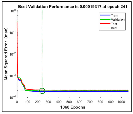
Figure 4.
Validation performance of the ANN.
The ANN resulted in an overall R2 value of 0.9996. The regression plot of the developed model is shown in Figure 5. Based on Figure 5, it was observed that the target output and line of best fit are in good correlation. This indicates that the ANN produces results that are very close to the desired output.
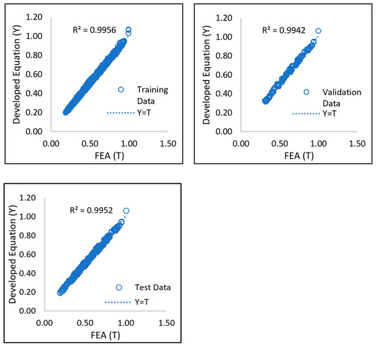
Figure 5.
Regression plot of the developed ANN for training, validation, and test phases.
The MAE, MSE, and R2 value of the model for each of the training, validation, and test phases are summarised in Table 9. Figure 6 represents the William’s plot of the ANN. As illustrated in Figure 6, the failure pressure data falls within the valid region of 0 < h < 0.01 and −3 < SR < 3. The implementation of the leverage strategy established the statistical validity of the developed model.
Table 9.
Mean absolute error (MAE), MSE, and R2 values of the model for training, validation, and test phase.
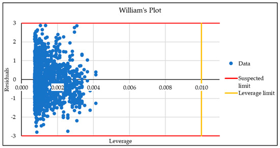
Figure 6.
William’s plot of the ANN model.
3.2. Development of the Empirical Equation
The empirical equation for the failure pressure prediction of circumferentially aligned interacting corrosion defects subjected to internal pressure and axial compressive stress is based on the representation of the developed ANN in matrix form. The developed equations have been organised into four steps to arrive at the failure pressure prediction of the corroded pipe with circumferentially aligned defects. The steps involved are summarised as follows.
Step 1: Calculation of the normalised effective length and depth of defect.
Step 2: Normalization of input parameters
Step 3: Calculation of the normalised output value.
Step 4: Calculation of failure pressure.
3.3. Evaluation of the Developed Empirical Failure Pressure Assessment Method
Based on Figure 7, it was observed that the predicted failure pressures obtained using the developed empirical equation are comparable to that of FEM. The maximum and minimum percentage differences observed are 0.98% and −9.92%, respectively. A positive percentage difference indicates overestimation. However, this overestimation is less than 1.00%; hence, it is negligible. In addition, only 1.70% of the 1353 datasets resulted in overestimation. The standard deviation of the results is 2.27, and the confidence level of the percentage error of predictions that are less than 9.92% is 99.9%, as the errors fall within four standard deviations of the mean.
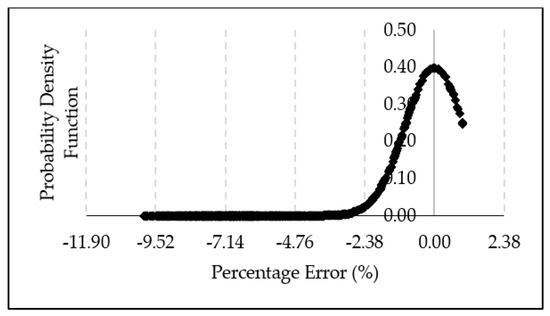
Figure 7.
Probability distribution of the percentage error obtained using the new empirical failure pressure assessment method and FEM based on the parameters of the ANN training data.
Since data on burst tests of corroded pipes subjected to combined loadings for interacting defects are limited, FEM was utilised to further verify the new prediction approach using a set of arbitrary data for API 5L X52, X65, and X80 material. Table 10 summarises the parametric details, failure pressure predictions using FEM, and the developed equation, as well as the percentage difference between the methods. Based on Table 10, the Root Mean Square Error (RMSE) of the failure pressure predictions is 0.05. This indicates a good correlation among the predictions obtained using FEM and the developed equations. The minimum and maximum percentage differences observed are −9.42% and −0.01%, respectively.
Table 10.
Percentage difference between the failure pressure obtained using FEA and the developed equation for arbitrary models.
The predicted failure pressures fall within the 99.9% confidence level for true ultimate tensile strength values of 612 MPa, 629 MPa, and 718 MPa, normalised defect spacings of 0.00 to 3.00, normalised effective defect lengths of 0.00 to 2.95, normalised effective defect depths of 0.00 to 0.80, and normalised axial compressive stress of 0.00 to 0.60. The equations resulted in minimal overestimations, while underestimated values were not overly conservative (within an error of 0.98%). Using these equations, a correlation between defect geometries and the failure pressure of API 5L X52, X65, and X80 with circumferentially aligned interacting corrosion defects subjected to internal pressure and axial compressive stress was established. This contributes to overcoming the limitations of the conventional assessment codes as the conventional codes do not cater for pipes with interacting defects subjected to combined loading. Furthermore, the developed ANN model in this study can be easily retrained using data for different materials to increase its robustness, and the equations can be revised accordingly, which can be useful for future research.
4. Extensive Parametric Studies Using the Developed Empirical Equation
Using the developed empirical equations, a parametric study was carried out to analyse the behaviour of API 5L X52 and X65 pipe grades for different combinations of geometric parameters. Generally, for API 5L X52 and X65 pipes, it was found that the normalised failure pressures overlap almost completely. However, the normalised failure pressures for X80 pipes are comparatively higher than that of the other two materials, as illustrated in Figure 8, Figure 9, Figure 10 and Figure 11.
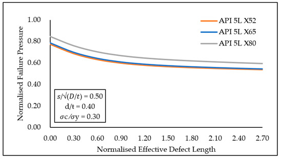
Figure 8.
Failure pressure predictions for API 5L X52, X65, and X80 pipe for multiple normalised effective defect lengths.
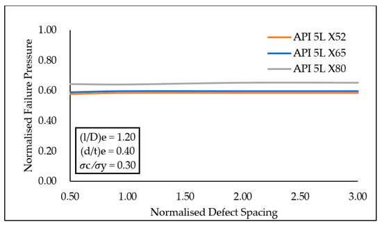
Figure 9.
Failure pressure predictions for API 5L X52, X65, and X80 pipe for multiple normalised defect spacings.
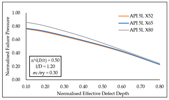
Figure 10.
Failure pressure predictions for API 5L X52, X65, and X80 pipes for multiple normalised effective defect depths.
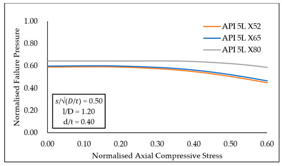
Figure 11.
Failure pressure predictions for API 5L X52, X65, and X80 pipes for multiple normalised axial compressive stress.
For the effects of normalised effective defect lengths and defect spacing, it was found that as the normalised effective defect length increases from 0.00 to 1.80 for a defect spacing of 0.50, normalised effective defect depth of 0.4, and a normalised axial compressive stress of 0.30, the failure pressure decreases gradually up to a maximum of 28.17% and begins to plateau beyond a normalised effective defect length of 1.80, as illustrated in Figure 8. This trend is observed for all other conditions as well.
Based on Figure 9, as the normalised defect spacing increases from 0.00 to 3.00 for a normalised effective defect length of 1.20, a normalised effective defect depth of 0.4, and a normalised axial compressive stress of 0.30, the failure pressure also increases (a maximum of 0.95%) due to the decrease in stress–strain overlapping regions. These results are consistent with the former literature [18,32,43]. Under all other geometric conditions, for a change in the parameters, the normalised failure pressures of API 5L X52 and X65 pipes are almost similar with a maximum percentage difference of 1.26%. However, the normalised failure pressure for high toughness pipe material is relatively larger, with a maximum percentage difference of 9.48%.
As for the effects of defect depth, as the defect depth increases from 0.10 to 0.80, the failure pressure of the corroded pipe drops drastically with a maximum decrease of 71.88% for a normalised defect spacing of 0.50, a normalised effective defect length of 1.2, and a normalised axial compressive stress of 0.30 for a high toughness pipe (API 5L X80). It was observed that, beyond a normalised effective defect depth of 0.60, the normalised failure pressure of the three pipe grades begins to converge and overlap, as illustrated in Figure 10. Under all other conditions, the normalised failure pressures of the three materials exhibit the same failure pressure trend.
It was observed that when a normalised axial compressive stress of larger than 0.60 was imposed on a corroded pipe, the pipe buckles. This is also the case for pipes subjected to an axial compressive stress of 0.60, with normalised effective defect depths of greater than 0.60. The normalised failure pressures of the pipe remain constant for a normalised axial compressive stress values of 0.00 to 0.40. Beyond that, the normalised failure pressure begins to reduce gradually with a maximum pressure drop of 31.57% observed for the API 5L X52 pipe of 0.50 normalised defect spacing, 1.20 normalised effective defect length, and 0.40 normalised defect depth, as illustrated in Figure 11.
In this study, the developed equation is accurate for API 5L X52, X65, and X80 pipes. However, the accuracy of the equation drops significantly (up to 30.00%) when applied to pipe grades that fall between the ranges of these materials, as the interval between the true ultimate tensile strength of high toughness and medium toughness pipe grades used in this study is large. To overcome this situation, future studies should consider using a greater number of ANN training dataset that consists of different types of materials with smaller true ultimate tensile strength intervals to increase the robustness of ANN.
5. Conclusions
In this study, an empirical equation to predict the failure pressure of API 5L X52, X65, and X80 pipes with circumferentially aligned interacting corrosion defects subjected to internal pressure and axial compressive stress as a function of true ultimate tensile strength, normalised defect spacing, depth and length, and axial compressive stress was developed. The new equations predicted failure pressures for these pipe grades with an R2 value of 0.99 and an error range of −9.92% to 0.98% for the normalised defect spacings of 0.00 to 3.00, normalised effective defect lengths of 0.00 to 2.95, normalised effective defect depths of 0.00 to 0.80, and normalised axial compressive stress of 0.00 to 0.60.
Based on the parametric study conducted, it was found that the low and medium toughness materials exhibit the same pipe failure patterns as the normalised failure pressure values of the pipe materials; they are almost similar. However, for high toughness materials, the normalised failure pressures are higher by a maximum of 9.48% than that of the low and medium toughness materials. The defect depth has the most significant influence on the failure pressure of a corroded pipeline with a maximum pressure drop of 68.90% followed by axial compressive stress (maximum pressure drop of 31.57%), defect length (maximum pressure drop of 28.17%), and the defect spacing (maximum pressure drop of 0.95%).
The proposed assessment method that incorporates combined loadings for the failure pressure prediction of API 5L X52, X65, and X80 pipelines with circumferentially aligned interacting corrosion defects overcomes the lack of an analytical closed-form solution for the failure pressure prediction of API 5L X52, X65, and X80 corroded pipelines subjected to combined loadings.
Supplementary Materials
The following supporting information can be downloaded at: https://www.mdpi.com/article/10.3390/app12094120/s1.
Author Contributions
Conceptualization, S.K. and M.O.; methodology, M.L. and S.D.V.K.; software, S.K.; validation, M.L., S.D.V.K. and S.K.; formal analysis, M.L., S.D.V.K. and S.K.; investigation, M.L. and S.D.V.K.; resources, S.K.; data curation, M.L., S.D.V.K. and S.K.; writing—original draft preparation, M.L. and S.D.V.K.; writing—review and editing, S.K. and M.O.; visualization, S.K. and M.O.; supervision, S.K.; project administration, S.K.; funding acquisition, S.K. All authors have read and agreed to the published version of the manuscript.
Funding
This work was supported by Yayasan Universiti Teknologi PETRONAS, Malaysia (015LC0-110) and the Ministry of Higher Education, Malaysia (FRGS/1/2018/TK03/UTP/02/1).
Conflicts of Interest
The authors declare no conflict of interest.
Nomenclature
| ANN | Artificial neural network |
| DOF | Degree of freedom |
| FEA | Finite element analysis |
| FEM | Finite element method |
| MAE | Mean absolute error |
| Pipe diameter | |
| Modulus of elasticity | |
| Pipe length | |
| Pipe failure pressure | |
| Normalised pipe failure pressure obtained using the newly developed equation | |
| Normalised pipe failure pressure obtained using FEM | |
| Pipe intact pressure | |
| Defect depth | |
| Input parameter value | |
| Maximum input parameter value | |
| Minimum input parameter value | |
| Normalised input parameter value | |
| Normalised maximum input parameter value | |
| Normalised minimum input parameter value | |
| Defect length | |
| Neuron in hidden layer | |
| Output parameter value | |
| Maximum output parameter value | |
| Minimum output parameter value | |
| Normalised output parameter value | |
| Normalised maximum output parameter value | |
| Normalised minimum output parameter value | |
| Pipe wall thickness | |
| Circumferential defect spacing | |
| Poisson’s ratio | |
| Defect width | |
| Ultimate tensile strength | |
| True ultimate tensile strength | |
| Yield stress |
References
- Ossai, C.I.; Boswell, B.; Davies, I. Application of Markov modelling and Monte Carlo simulation technique in failure probability estimation—A consideration of corrosion defects of internally corroded pipelines. Eng. Fail. Anal. 2016, 68, 159–171. [Google Scholar] [CrossRef]
- Arumugam, T.; Karuppanan, S.; Ovinis, M. Finite element analyses of corroded pipeline with single defect subjected to internal pressure and axial compressive stress. Mar. Struct. 2020, 72, 102746. [Google Scholar] [CrossRef]
- Choi, J.; Goo, B.; Kim, J.; Kim, Y.; Kim, W. Development of limit load solutions for corroded gas pipelines. Int. J. Press. Vessel. Pip. 2003, 80, 121–128. [Google Scholar] [CrossRef]
- Lo, M.; Karuppanan, S.; Ovinis, M. Failure Pressure Prediction of a Corroded Pipeline with Longitudinally Interacting Corrosion Defects Subjected to Combined Loadings Using FEM and ANN. J. Mar. Sci. Eng. 2021, 9, 281. [Google Scholar] [CrossRef]
- Lee, Y.; Kim, Y.P.; Moon, M.; Bang, W.H.; Oh, K.H.; Kim, W.S. The Prediction of Failure Pressure of Gas Pipeline with Multi Corroded Region. Mater. Sci. Forum 2005, 475–479, 3323–3326. [Google Scholar] [CrossRef]
- Kumar, S.V.; Karuppanan, S.; Ovinis, M. Failure Pressure Prediction of High Toughness Pipeline with a Single Corrosion Defect Subjected to Combined Loadings Using Artificial Neural Network (ANN). Metals 2021, 11, 373. [Google Scholar] [CrossRef]
- Kumar, S.D.V.; Karuppanan, S.; Ovinis, M. An Empirical Equation for Failure Pressure Prediction of High Toughness Pipeline with Interacting Corrosion Defects Subjected to Combined Loadings Based on Artificial Neural Network. Mathematics 2021, 9, 2582. [Google Scholar] [CrossRef]
- Belachew, C.T.; Ismail, M.C.; Karuppanan, S. Burst Strength Analysis of Corroded Pipelines by Finite Element Method. J. Appl. Sci. 2011, 11, 1845–1850. [Google Scholar] [CrossRef][Green Version]
- Chen, Y.; Zhang, H.; Zhang, J.; Liu, X.; Li, X.; Zhou, J. Failure assessment of X80 pipeline with interacting corrosion defects. Eng. Fail. Anal. 2015, 47, 67–76. [Google Scholar] [CrossRef]
- De Andrade, E.Q.; Benjamin, A.C.; Machado, P.R.S.; Pereira, L.C.; Jacob, B.; Carneiro, E.G.; Guerreiro, J.N.C.; Silva, R.C.C.; Noronha, D.B. Finite Element Modeling of the Failure Behavior of Pipelines Containing Interacting Corrosion Defects. In Proceedings of the International Conference on Offshore Mechanics and Arctic Engineering-OMAE, Hamburg, Germany, 4–9 June 2006; pp. 315–325. [Google Scholar] [CrossRef]
- Fatoba, O.; Akid, R. Low Cycle Fatigue Behaviour of API 5L X65 Pipeline Steel at Room Temperature. Procedia Eng. 2014, 74, 279–286. [Google Scholar] [CrossRef]
- DNV. Recommended Practice DNV-RP-F101; no. May; DNV: Oslo, Norway, 2017. [Google Scholar]
- Chiodo, M.S.; Ruggieri, C. Failure assessments of corroded pipelines with axial defects using stress-based criteria: Numerical studies and verification analyses. Int. J. Press. Vessel. Pip. 2009, 86, 164–176. [Google Scholar] [CrossRef]
- Cosham, A.; Hopkins, P. The Assessment of Corrosion in Pipeline-Guidance in the Pipeline Defect Assessment Manual (PDAM). In Proceedings of the Pipeline Pigging and Integrity Management Conference, Amsterdam, The Netherlands, 17–18 May 2004; pp. 1–18. [Google Scholar]
- Cosham, A.; Hopkins, P.; Macdonald, K. Best practice for the assessment of defects in pipelines—Corrosion. Eng. Fail. Anal. 2007, 14, 1245–1265. [Google Scholar] [CrossRef]
- Netto, T.A.; Ferraz, U.; Estefen, S. The effect of corrosion defects on the burst pressure of pipelines. J. Constr. Steel Res. 2005, 61, 1185–1204. [Google Scholar] [CrossRef]
- Chauhan, V.; Swankie, T.D.; Espiner, R.; Wood, I. Developments in Methods for Assessing the Remaining Strength of Corroded Pipelines. In Proceedings of the NACE Corrosion 2009 Conference Expo, Houston, TX, USA, 4–7 November 2009; No. 09115. pp. 1–29. [Google Scholar]
- Li, X.; Bai, Y.; Su, C.; Li, M. Effect of interaction between corrosion defects on failure pressure of thin wall steel pipeline. Int. J. Press. Vessel. Pip. 2016, 138, 8–18. [Google Scholar] [CrossRef]
- Zangenehmadar, Z.; Moselhi, O. Assessment of Remaining Useful Life of Pipelines Using Different Artificial Neural Networks Models. J. Perform. Constr. Facil. 2016, 30, 4016032. [Google Scholar] [CrossRef]
- Liu, X.; Xia, M.; Bolati, D.; Liu, J.; Zheng, Q.; Zhang, H. An ANN-based failure pressure prediction method for buried high-strength pipes with stray current corrosion defect. Energy Sci. Eng. 2019, 8, 248–259. [Google Scholar] [CrossRef]
- Hagan, M.T.; Menhaj, M.B. Training feedforward networks with the Marquardt algorithm. IEEE Trans. Neural Netw. 1994, 5, 989–993. [Google Scholar] [CrossRef]
- Shirzad, A.; Tabesh, M.; Farmani, R. A comparison between performance of support vector regression and artificial neural network in prediction of pipe burst rate in water distribution networks. KSCE J. Civ. Eng. 2014, 18, 941–948. [Google Scholar] [CrossRef]
- El-Abbasy, M.S.; Senouci, A.; Zayed, T.; Mirahadi, F.; Parvizsedghy, L. Artificial neural network models for predicting condition of offshore oil and gas pipelines. Autom. Constr. 2014, 45, 50–65. [Google Scholar] [CrossRef]
- Shuai, Y.; Shuai, J.; Xu, K. Probabilistic analysis of corroded pipelines based on a new failure pressure model. Eng. Fail. Anal. 2017, 81, 216–233. [Google Scholar] [CrossRef]
- Tohidi, S.; Sharifi, Y. Load-carrying capacity of locally corroded steel plate girder ends using artificial neural network. Thin-Walled Struct. 2016, 100, 48–61. [Google Scholar] [CrossRef]
- Sun, J.; Cheng, Y.F. Assessment by finite element modeling of the interaction of multiple corrosion defects and the effect on failure pressure of corroded pipelines. Eng. Struct. 2018, 165, 278–286. [Google Scholar] [CrossRef]
- Dongshan, Z. Residual Strength Calculation & Residual Life Prediction of General Corrosion Pipeline. Procedia Eng. 2014, 94, 52–57. [Google Scholar] [CrossRef]
- Soares, E.; Bruère, V.M.; Afonso, S.M.; Willmersdorf, R.B.; Lyra, P.R.; Bouchonneau, N. Structural integrity analysis of pipelines with interacting corrosion defects by multiphysics modeling. Eng. Fail. Anal. 2019, 97, 91–102. [Google Scholar] [CrossRef]
- Kumar, S.D.V.; Karuppanan, S.; Ovinis, M. Artificial Neural Network-Based Failure Pressure Prediction of API 5L X80 Pipeline with Circumferentially Aligned Interacting Corrosion Defects Subjected to Combined Loadings. Materials 2022, 15, 2259. [Google Scholar] [CrossRef]
- Arumugam, T.; Rosli, M.K.A.M.; Karuppanan, S.; Ovinis, M.; Lo, M. Burst capacity analysis of pipeline with multiple longitudinally aligned interacting corrosion defects subjected to internal pressure and axial compressive stress. SN Appl. Sci. 2020, 2, 1201. [Google Scholar] [CrossRef]
- ANSYS. ANSYS Theory Reference; ANSYS Inc.: Canonsburg, PA, USA, 2019. [Google Scholar]
- Wang, Y.-L.; Li, C.-M.; Chang, R.-R.; Huang, H.-R. State evaluation of a corroded pipeline. J. Mar. Eng. Technol. 2016, 15, 88–96. [Google Scholar] [CrossRef]
- Wiesner, C.; Maddox, S.; Xu, W.; Webster, G.; Burdekin, F.; Andrews, R.; Harrison, J. Engineering critical analyses to BS 7910—The UK guide on methods for assessing the acceptability of flaws in metallic structures. Int. J. Press. Vessel. Pip. 2000, 77, 883–893. [Google Scholar] [CrossRef]
- Cronin, D.; Pick, R.J. Prediction of the failure pressure for complex corrosion defects. Int. J. Press. Vessel. Pip. 2002, 79, 279–287. [Google Scholar] [CrossRef]
- Terán, G.; Capula-Colindres, S.; Velázquez, J.C.; Fernández-Cueto, M.J.; Angeles-Herrera, D.; Herrera-Hernández, H. Failure Pressure Estimations for Pipes with Combined Corrosion Defects on the External Surface: A Comparative Study. Int. J. Electrochem. Sci. 2017, 12, 10152–10176. [Google Scholar] [CrossRef]
- Bjørnøy, O.H.; Sigurdsson, G.; Cramer, E. Residual Strength of Corroded Pipelines, DNV Test Results. In Proceedings of the Tenth (2000) International Offshore and Polar Engineering Conference, Seattle, WA, USA, 28 May–2 June 2000; Volume II, pp. 1–7. [Google Scholar]
- Benjamin, A.C.; Freire, J.L.F.; Vieira, R.D.; Diniz, J.L.C.; de Andrade, E.Q. Burst Tests on Pipeline Containing Interacting Corrosion Defects. In Proceedings of the 24th International Conference on Offshore Mechanics and Arctic Engineering (OMAE 2005), Halkidiki, Greece, 12–17 June 2005; Volume 3, pp. 403–417. [Google Scholar] [CrossRef]
- Чин, К.Т.; Арумугам, Т.; Каруппанан, С.; Овинис, М. Failure pressure prediction of pipeline with single corrosion defect using artificial neural network. Sci. Technol. OIL OIL Prod. Pipeline Transp. 2021, 4, 10–17. [Google Scholar] [CrossRef]
- Xu, W.Z.; Li, C.B.; Choung, J.; Lee, J.M. Corroded pipeline failure analysis using artificial neural network scheme. Adv. Eng. Softw. 2017, 112, 255–266. [Google Scholar] [CrossRef]
- Gurney, K. An Introduction to Neural Networks; UCL Press: London, UK, 1997. [Google Scholar]
- Atta, M.M.; Abd-Elhady, A.; Abu-Sinna, A.; Sallam, H. Prediction of failure stages for double lap joints using finite element analysis and artificial neural networks. Eng. Fail. Anal. 2019, 97, 242–257. [Google Scholar] [CrossRef]
- Kumar, S.D.V.; Kai, M.L.Y.; Arumugam, T.; Karuppanan, S. A Review of Finite Element Analysis and Artificial Neural Networks as Failure Pressure Prediction Tools for Corroded Pipelines. Materials 2021, 14, 6135. [Google Scholar] [CrossRef] [PubMed]
- Alang, N.A.; Razak, N.A.; Shafie, K.A.; Sulaiman, A. Finite Element Analysis on Burst Pressure of Steel Pipes with Corrosion Defects. In Proceedings of the 13th International Conference on Fracture, Beijing, China, 16–21 June 2013; no. 1. pp. 1–10. [Google Scholar]


Publisher’s Note: MDPI stays neutral with regard to jurisdictional claims in published maps and institutional affiliations. |
© 2022 by the authors. Licensee MDPI, Basel, Switzerland. This article is an open access article distributed under the terms and conditions of the Creative Commons Attribution (CC BY) license (https://creativecommons.org/licenses/by/4.0/).