Hierarchy Establishment from Nonlinear Social Interactions and Metabolic Costs: An Application to Harpegnathos saltator

Abstract

Social hierarchies are ubiquitous in social groups such as human societies and social insect colonies; however, the factors that maintain these hierarchies are less clear. Motivated by the shared reproductive hierarchy of the ant species Harpegnathos saltator, we have developed simple compartmental nonlinear differential equations to explore how key life-history and metabolic rate parameters may impact and determine its colony size and the length of its shared hierarchy. Our modeling approach incorporates nonlinear social interactions and metabolic theory. The results from the proposed model, which were linked with limited data, show that: (1) the proportion of reproductive individuals decreases over colony growth; (2) an increase in mortality rates can diminish colony size but may also increase the proportion of reproductive individuals; and (3) the metabolic rates have a major impact in the colony size and structure of a shared hierarchy.

1. Introduction

Animals live in social groups to obtain collective benefits like improved foraging, predator evasion, and brood care [1]. Hierarchies within a group allow individuals with higher status to enjoy a greater share of resources than those with lower status [2]. While theoretical and empirical work has provided insight into how hierarchies are established [3], different strategies may govern the stability of their resulting structure [4,5]. Within animal taxa, the structures of these hierarchies can take linear or non-linear forms. A linear hierarchy occurs when each group member occupies a single rank and is subordinate to those ranked above them and dominant to those ranked below [6,7]. Not all hierarchies in nature are linear. For example, there are despotic hierarchies where a single individual monopolizes power over a group of subordinates [7,8,9,10], and shared dominance structures where multiple individuals occupy a single rank [11]. We say that a group presents a non-linear hierarchy if a shared hierarchy is present in the group. Some taxa, including humans, show a shared (non-linear) hierarchy, where a group of dominant individuals presides over many subordinates [11].

In eusocial colonies, some members are reproductive, while others are not. In this way, the distribution of reproduction among the population is skewed by the many individuals who are reproductive [12]. The allocation of individuals in the colony to reproduction forms hierarchies in several species, where those holding a reproductive role have a higher rank, and those who are not reproductive occupy subordinate ranks [6]. For instance, in the ant species Harpegnathos saltator, the privilege of reproduction (for a certain subgroup inside its colony) generates a nonlinear social hierarchy, i.e., a ranking. Other examples of shared hierarchies are in the queenless colonies of the Ponerine ant, Pseudoneoponera tridentata, Gnamptogenys menadensis, and Rhytidoponera confusa, where certain mated workers can become reproductively active members, known as gamergates [7,13,14].

Previous mathematical models dealing with hierarchy establishment have used probabilistic and game theory approaches with emphasis on dominance hierarchy. Dominance hierarchy is a form of animal social structure in which a linear or nearly linear ranking exists. Monnin et al. (1999) constructed a probabilistic model using the inclusive-fitness model (that is, the fitness of the colony/cost of becoming dominant is greater than the benefits), combined with alpha replacement with different types of near-linear hierarchies [15]. They looked into a critical rank at which ants enter the reproductive hierarchy and the length of that hierarchy. Cant et al. (2005) extended their previous model dealing with kin selection to quantify the helping effort and see how relatedness plays a role in hierarchical development [16]. They found that lower ranks work harder at raising the young than higher up ranks do, that helpers work less hard in larger groups, and that the productivity will increase with relatedness between group members. Furthermore, Broom et al. (2002) modeled dominance hierarchy, starting from a group with no established order, as a multi-player game through game theory [17]. Using the classic Dove–Hawk model and Swiss tournament rules, they found that when a majority of resources go to the few of the top hierarchy, the final contests of top individuals become violent, while the final contests of lower-ranked individuals are peaceful. Later, Broom (2002) proposed a general unified model of dominance hierarchy using evolutionary game theory where he investigated how the hierarchies were formed and maintained [4]. Beaugrand (1997) created a simulation model to see how hierarchies were formed concerning individual differences and how it affected the transitive property of dominance for the animal’s resource holding potential [18]. He found that a carry-over effect may explain why there are differences in predicted hierarchies in contrast with observed hierarchies; when individual differences in the group members are significant, they lead to a winner–loser/carry-over effect (successive victories lead to more victories and vice versa).

Social dominance hierarchies are widespread with most attention on linear and despotic hierarchies. However, little is known about the mechanisms that produce nonlinear structures, especially shared hierarchies [7]. To our best knowledge, the available work on this topic has been done by Sasaki et al. [7]. In this study, agent-based models, combined with experimental data on the ant species H. Saltator, were used to predict the emergence of complex animal hierarchies including shared hierarchies. Their computer simulations show that a linear hierarchy emerges when a typical winner–loser interaction (dominance biting of H. Saltator) is present; a despotic hierarchy emerges when a policing interaction is added; and a shared hierarchy emerges with the addition of a winner-winner interaction that results in a positive outcome for both interactors (antennal dueling). The model developed by Sasaki et al. [7] provides a baseline for us to build mathematical tractable models that can explore the impacts of the colony size and metabolic rates on the establishment of shared hierarchies.

A metabolic theory of ecology suggests that increased group size reduces overall metabolic costs, thereby increasing the efficiency of the group [19,20]. Studies [21,22,23,24] show that colony size (the group size of worker ants) affects parameters across different taxa, (e.g., metabolic rates), such that these parameters scale with colony size. For instance, the number of reproductive individuals in multiple ant species has been shown to be a function of the number of workers elevated to an exponent less than one. In addition, the number of reproductives per capita decreases with the size of mature colonies across some species [23]. Temnothorax ants, in the laboratory, show a colony size scaling as lower per capita brood production and lower energy consumption occur at larger colony sizes [24]. In the ant P. occidentalis, the biomass of reproduction does not scale with colony size, but the probability of producing a reproductive individual increases with colony size [25]. This scaling phenomenon is not considered in the approach proposed by Sasaki et al. [7] since their computational results are based on fixed colony size. So, there is a need to develop a simple mathematical model to explore the impacts of colony size and the related metabolic theory of ecology on shaping shared social hierarchy.

Motivated by the ant species Harpegnathos saltator and the work by Sasaki et al. [7], we develop a mechanistic-based but mathematical tractable model to understand how the shared hierarchy inside a colony, reflected by the ratio of reproductive workers to all workers, impacts the population dynamics and structure of social insect colonies. Our proposed model incorporates nonlinear social interactions and the related metabolic rate influenced by hierarchy establishment. We expect our proposed model provides insight into the role of colony size in shaping shared hierarchy.

The paper is organized as follows: In Section 2, we start with the biological background of the particular ant species H. Saltator which motivates our work, and then we formulate a mathematical model based on ecological assumptions that are supported by data and literature. In Section 3, we perform mathematical analyses of the proposed model. In Section 4, we compare model simulations to data on colony size and reproductive ratio for laboratory-observed H. Saltator colonies. We also perform parameter estimation and bifurcation analysis for the proposed model. Finally, in Section 5, we summarize our results and elaborate on the implications of our model and potential future work.

2. Model Formulation

Motivated by the work of queenless colonies of the Ponerine ant, Harpegnathos saltator [7], we derive our model on its shared hierarchy. A Harpegnathos saltator ant’s life cycle consists of four stages: egg, larva, pupa, and adult. Fertilized eggs become female ants (queens and workers), whereas unfertilized eggs develop into male ants. The period from egg to adult can last over 79 days [26]. The average Harpegnathos worker lives from 200 to 400 days in the lab, while the ecological factors in the field reduce this life span [27]. In contrast, a reproductive queen can live for more than 5 years in the laboratory [28]; however, it is estimated that she may only live for as long as 1.79 years in the field [29]. Single individual queens establish new colonies as foundresses. After constructing a nest, a queen then produces and cares for eggs, which grow into larvae, pupae, and finally workers. In this species, a foundress hunts above ground to feed her first offspring. This continues until adult workers take over brood care, nest construction, and foraging. However, when the queen senesces and/or dies, she is replaced by gamergates (reproductive workers) who partition their reproduction among one another evenly [13,30]. Most gamergates lose their status through senescence and death, although some may revert to worker-like behavior and physiology in the laboratory [31].

While queens and workers of H. Saltator show morphological differences, non-reproductive workers also exhibit distinct behaviors such as rapid locomotion, hunting and handling of live arthropods, and low posture that differ from gamergates who show slow locomotion, high posture, and egg-laying [32]. Since any adult worker can become a gamergate, all can be categorized as potential gamergates during the establishment of a new reproductive hierarchy [33]. Over time, the shared nonlinear hierarchy is established through potential chemical cues and social interactions, such as policing, antennal dueling, and dominance biting. These interactions eventually divide the colony into two classes based on reproduction: established gamergates and non-reproductive workers [7]. Established gamergates are defined as gamergates who maintain their social position in the hierarchy.

This specific biological background provides us with a template for mathematical modeling. We denote $N_g\left(t\right)$ as the number of established gamergates, $N_w\left(t\right)$ denotes the number of non-reproductive workers, and $N\left(t\right)=N_g\left(t\right)+N_w\left(t\right)$ represents the total population size of female adult ants (colony size) at time t (days). We develop a mechanistic model based on nonlinear social interactions and metabolic theory to explore how life-history parameters and the related metabolic costs shape the hierarchy structure of a social insect colony. Ecological assumptions of our generalized model are as follows:

(a)

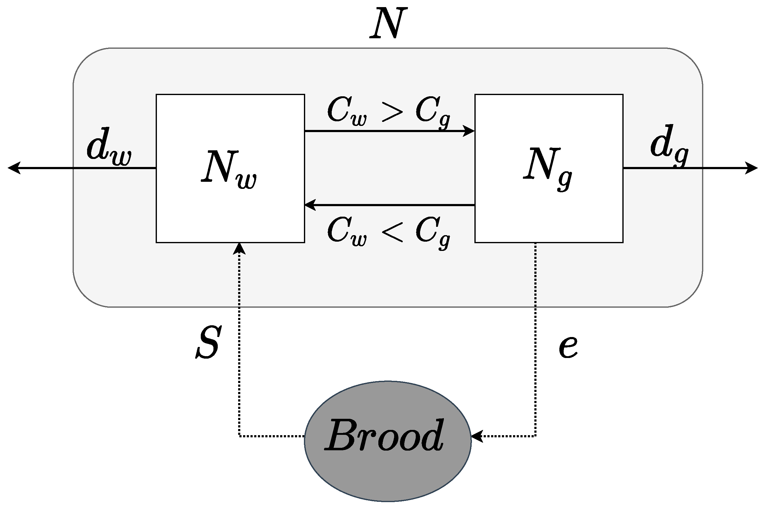
Modeling Relative Cost: Assuming that gamergates are the only members of the colony who actively reproduce, the cost for all gamergates of remaining in their status in the colony is measured by $E_g$ (Kcal) which consists of the energy cost of laying eggs as well as the energy to perform behaviors that maintain the social hierarchy such as antennal dueling and dominance behaviors. According to the ecological metabolism theory, the formulation of $E_g$ is modeled by

$$E_g={\beta }_g{N}_g^{{\delta }_g},$$

where ${\beta }_g$ is a normalization constant (measured in microwatts per gram μW/gr). This coefficient ${\beta }_g$ corresponds to the variation in metabolic rates across gamergates in the group. Then, ${\delta }_g$ is a scaling exponent, which describes how fast the cost/metabolic rate changes with respect to the biomass of the group of gamergates [34]. If ${\delta }_g<1$, then the metabolic rate of the group grows slower than the biomass. Instead, if ${\delta }_g>1$ the metabolic rate of the group grows faster than the biomass. From the literature, the values of ${\delta }_g$ for social insects (e.g., ants) should be in the range 0–1.75 [20,35]. Adopting a similar modeling approach for the non-reproductive worker population, the cost of all non-reproductive workers $N_w$ to maintain their status in the colony is $E_w$, given by

$$E_w={\beta }_n{N}^{{\delta }_n},$$

which includes the energy cost of providing resources for the whole colony, such as brood care, foraging, etc. We assume that $E_w$ is proportional to the total colony size N as the non-reproductive workers take care of the whole colony (and not just themselves, unlike gamergates). Based on their faster relative speed [32], non-reproductive workers most likely have a higher metabolic cost compared to gamergates [27], i.e., ${\delta }_n\ge {\delta }_g$. Therefore, the relative cost for gamergates is defined by

$${\displaystyle C_g=\frac{E_g}{E_g+E_w}=\frac{{\beta }_g{N}_g^{{\delta }_g}}{{\beta }_g{N}_g^{{\delta }_g}+{\beta }_n{N}^{{\delta }_n}}.}$$

(1)

Applying the similar arguments to non-reproductive workers $N_w$, their relative cost is defined as

$$\begin{array}{ccc}\hfill C_w& :=& \frac{E_w}{E_g+E_w}=\frac{{\beta }_n{N}^{{\delta }_n}}{{\beta }_g{N}_g^{{\delta }_g}+{\beta }_n{N}^{{\delta }_n}}\hfill \end{array}$$

Note that $C_g+C_w=1$

(b)

Colony Size N: Let e be the average number of eggs produced per gamergate, then the total number of eggs produced at time t would be $e{N}_g\left(t\right)$. The survival of eggs is directly linked to the care provided by the number of non-reproductive workers [32]. Thus, we assume that the survival rate of eggs is proportional to the relative cost of the worker class $C_w$. Therefore, the input of new members is obtained as follows

$$\mathrm{New} \mathrm{Colony} \mathrm{Members}=\frac{e{\beta }_n{N}^{{\delta }_n}}{{\beta }_g{N}_g^{{\delta }_g}+{\beta }_n{N}^{{\delta }_n}}{N}_g.$$

(2)

We assume that the colony has a density-dependent mortality rate due to limited resources, given by

$$\mu =(d_w{N}_w+d_g{N}_g)$$

(3)

where $d_w$ and $d_g$ represent the mortality rate of workers and gamergates, respectively. Therefore, the colony size is modeled as follows

$$\begin{array}{ccc}\hfill \frac{dN}{dt}& =& \underset{\mathrm{survival}\mathrm{rate}}{\underbrace{\frac{{\beta }_n{N}^{{\delta }_n}}{{\beta }_g{N}_g^{{\delta }_g}+{\beta }_n{N}^{{\delta }_n}}}}\underset{\mathrm{eggs}}{\underbrace{e{N}_g}}-\underset{\mathrm{density}\mathrm{depend}\mathrm{mortality}\mathrm{rate}}{\underbrace{\left(d_w{N}_w+d_g{N}_g\right)}}N\hfill \end{array}$$

(c)

Gamergates $N_g$ and Workers $N_w$: We adopt the concept of [15] to model that a non-reproductive worker would leave its worker status and enter into the gamergate phase when the worker’s relative cost $C_w$ is higher than the gamergate’s relative cost $C_g$, and vice versa [15,32]. Since it has been shown that gamergates can revert to worker status [31] and non-reproductive workers can become gamergates [33], we assume that an ant can interchange between a gamergate and non-reproductive worker status based on the relative cost of remaining in a particular group. This relative cost derives from metabolic costs and is also related to its contribution to colony function. Thus, the population dynamics of gamergates is modeled as follows

$$\begin{array}{ccc}\hfill \frac{d{N}_g}{dt}& =& \underset{\mathrm{switch}\mathrm{from}\mathrm{worker}\mathrm{to}\mathrm{gamergates}}{\underbrace{max\{C_w-C_g,0\}{N}_w}}-\underset{\mathrm{switch}\mathrm{from}\mathrm{gamergates}\mathrm{to}\mathrm{worker}}{\underbrace{max\{C_g-C_w,0\}{N}_g}}-\underset{\mathrm{Mortality}}{\underbrace{d_{g}N{N}_g}}\hfill \end{array}$$

(4)

To model the non-reproductive workers’ population dynamics, we assume that all newborns are in the non-reproductive worker status first, with the possibility of transitioning into the status of gamergates. We apply a similar approach as above so that the population dynamics of non-reproductive workers is given by

$$\begin{array}{ccc}\hfill \frac{d{N}_w}{dt}& =& \underset{\mathrm{newborn}}{\underbrace{\frac{e{N}_g{\beta }_n{N}^{{\delta }_n}}{{\beta }_g{N}_g^{{\delta }_g}+{\beta }_n{N}^{{\delta }_n}}}}+\underset{\mathrm{switch}\mathrm{from}\mathrm{gamergates}\mathrm{to}\mathrm{worker}}{\underbrace{max\{C_g-C_w,0\}{N}_g}}\hfill \\ & & -\underset{\mathrm{switch}\mathrm{from}\mathrm{worker}\mathrm{to}\mathrm{gamergates}}{\underbrace{max\{C_w-C_g,0\}{N}_w}}-\underset{\mathrm{Mortality}}{\underbrace{d_{w}N{N}_w}}\hfill \end{array}$$

(5)

We provide the flow diagram of our mathematical model in Figure 1 and the related parameters in

Table 1. Biological meanings, best-fit values, ranges, and references for the parameters of the system (9) and (10).

Parameter	Description	Best Estimation	Range	Units	Reference
e	Egg-laying rate	2.42	$[0.5,2.42]$	eggs/day	Estimated
$d_g$	Natural death rate of gamergates	0.00028	$[0.0001,0.0025]$	$1/\mathrm{day}$	[27]
$d_w$	Natural death rate of workers	0.0025	$[0.0025,0.005]$	$1/\mathrm{day}$	[27]
${\beta }_g$	Normalized metabolic rates for gamergates	33.00	$[25,50]$	$\mathsf{\mu }\mathrm{W}/\mathrm{gr}$	Assumed
${\beta }_n$	Normalized metabolic rates for workers	74.60	$[45,150]$	$\mathsf{\mu }\mathrm{W}/\mathrm{gr}$	Assumed
${\delta }_g$	Hypometric relation factor of gamergates	0.99	$[0,2]$	1	Assumed
${\delta }_n$	Hypometric relation factor of workers	0.261	$[0,1]$	1	Assumed

. Based on the discussions above, we have the following nonlinear equations to model nonlinear hierarchy in social insect colonies:

$$\begin{array}{ccc}\hfill \frac{dN}{dt}& =& \frac{{\beta }_n{N}^{{\delta }_n}}{{\beta }_g{N}_g^{{\delta }_g}+{\beta }_n{N}^{{\delta }_n}}e{N}_g-\left(d_w{N}_w+d_g{N}_g\right)N\hfill \end{array}$$

(6)

$$\begin{array}{ccc}\hfill \frac{d{N}_w}{dt}& =& e{N}_g\frac{{\beta }_n{N}^{{\delta }_n}}{{\beta }_g{N}_g^{{\delta }_g}+{\beta }_n{N}^{{\delta }_n}}+N_{g}max\{C_g-C_w,0\}-N_{w}max\{C_w-C_g,0\}-d_w{N}_{w}N\hfill \end{array}$$

(7)

$$\begin{array}{ccc}\hfill \frac{d{N}_g}{dt}& =& N_{w}max\{C_w-C_g,0\}-N_{g}max\{C_g-C_w,0\}-d_g{N}_{g}N\hfill \end{array}$$

(8)

Remark 1.

The addition of relative costs is the unity, i.e., $C_w+C_g=1$, with all costs being non-negative [36,37]. The values of $C_w,C_g$ could determine the survival rate of eggs (e.g., brood care, foraging), and the interchangeable rate between gamergates and workers, [32]. Because non-reproductive workers perform risky tasks such as foraging, while gamergates remain in the nest and produce brood [38,39], it would be reasonable to assume that $d_w>d_g$, i.e., the mortality rate of workers is larger than that of gamergates.

Notice that $N_w=N-N_g$, so that we can reduce our proposed system (6)–(8) to the following two equations:

$$\begin{array}{ccc}\hfill \frac{dN}{dt}& =& e{N}_g\frac{{\beta }_n{N}^{{\delta }_n}}{{\beta }_g{N}_g^{{\delta }_g}+{\beta }_n{N}^{{\delta }_n}}-d_g{N}_{g}N-d_w(N-N_g)N\hfill \end{array}$$

(9)

$$\begin{array}{ccc}\hfill \frac{d{N}_g}{dt}& =& (N-N_g)max\{C_w-C_g,0\}-N_{g}max\{C_g-C_w,0\}-d_g{N}_{g}N\hfill \end{array}$$

(10)

which allows us to explore the following research questions theoretically:

• What are the key life-history parameters that determine the dynamics of the different classes in the colony $N,N_g,N_w$?
• How do the metabolic parameters, such as ${\beta }_g,{\beta }_n$, and the exponent parameters ${\delta }_g,{\delta }_n$ affect the colony size, N, and the size of the reproductive class $N_g$?
• How do the colony size, N, and the number of established gamergates, $N_g$, regulate each other?

3. Mathematical Analysis

Based on the formulation of Model (9) and (10), we observe that if $N=0$, then the system automatically has $N_g=N_w=0$ as $N=N_g+N_w$. At the same time, the expression of the metabolic cost $C_w$ and $C_g$ is not well defined at $N=0$. For convenience, by using the compactness concept, we define the following:

$$\begin{array}{c}\hfill \frac{dN}{dt}{|}_{N=0}=0 \mathrm{and} \frac{d{N}_g}{dt}{|}_{N=0}=0.\end{array}$$

(11)

Thus, we provide the following basic properties of the system (9) and (10):

Theorem 1.

The system (9) and (10) is positive invariant and bounded in ${\mathbb{R}}^{+2}$.

Notes: Theorem 1 implies that our proposed system (9) and (10) is well-defined biologically.

The first step to study the system (9) and (10) is to solve its steady states, i.e., equilibrium. According to (11), we can conclude that $N=N_g=0$ is always an equilibrium of the system (9) and (10). Moreover, this equilibrium is unstable.

Let us look at its interior equilibrium $(N^{*},N_g^{*})$. From the biological point of view, at the equilibrium the relative cost do not change and also the relative cost of workers is larger than that for gamergates.

For convenience, let us define the reproductive ratio ${\displaystyle X=\frac{N_g}{N}}$. Then by letting ${\displaystyle \frac{dN}{dt}=\frac{d{N}_g}{dt}=0}$, we obtain the following two equations:

$$\begin{array}{ccc}\hfill 0& =& e{N}_g\frac{{\beta }_n{N}^{{\delta }_n}}{{\beta }_g{N}_g^{{\delta }_g}+{\beta }_n{N}^{{\delta }_n}}-d_g{N}_{g}N-d_w(N-N_g)N\hfill \end{array}$$

(12)

$$\begin{array}{ccc}\hfill 0& =& (N-N_g)\frac{{\beta }_n{N}^{{\delta }_n}-{\beta }_g{N}_g^{{\delta }_g}}{{\beta }_n{N}^{{\delta }_n}+{\beta }_g{N}_g^{{\delta }_g}}-d_g{N}_{g}N\hfill \end{array}$$

(13)

Suppose $N_g,N\ne 0$. Dividing (12) by $N^2$ and letting $X=\frac{N_g}{N}$, we have the following equation:

$$0=eX\frac{{\beta }_n{N}^{{\delta }_n-1}}{{\beta }_g{\left(NX\right)}^{{\delta }_g}+{\beta }_n{N}^{{\delta }_n}}-d_{g}X-d_w+d_{w}X$$

Simplifying it further, we obtain this expression:

$$\frac{{\beta }_n{N}^{{\delta }_n-1}}{{\beta }_g{\left(NX\right)}^{{\delta }_g}+{\beta }_n{N}^{{\delta }_n}}=\frac{d_{g}X+d_w(1-X)}{eX}=\frac{d_g-d_w}{e}+\frac{d_w}{eX}$$

which gives

$$\begin{array}{c}\hfill \frac{{\beta }_n{N}^{{\delta }_n}}{{\beta }_g{\left(NX\right)}^{{\delta }_g}+{\beta }_n{N}^{{\delta }_n}}=N\left[\frac{d_g-d_w}{e}+\frac{d_w}{eX}\right].\end{array}$$

(14)

Notice that

$$\frac{{\beta }_n{N}^{{\delta }_n}-{\beta }_g{N}_g^{{\delta }_g}}{{\beta }_n{N}^{{\delta }_n}+{\beta }_g{N}_g^{{\delta }_g}}=\frac{2{\beta }_n{N}^{{\delta }_n}}{{\beta }_n{N}^{{\delta }_n}+{\beta }_g{N}_g^{{\delta }_g}}-1.$$

Based on (13), then we obtain the following equation:

$$\frac{2{\beta }_n{N}^{{\delta }_n}}{{\beta }_n{N}^{{\delta }_n}+{\beta }_g{N}_g^{{\delta }_g}}-1=\frac{d_{g}NX}{1-X}$$

which gives

$$\begin{array}{c}\hfill \frac{{\beta }_n{N}^{{\delta }_n}}{{\beta }_g{\left(NX\right)}^{{\delta }_g}+{\beta }_n{N}^{{\delta }_n}}=\frac{d_{g}NX}{2(1-X)}+1/2.\end{array}$$

(15)

Therefore, from (14), we have the following

$$N\left[\frac{d_g-d_w}{e}+\frac{d_w}{eX}\right]=\frac{d_{g}NX}{2(1-X)}+1/2.$$

It follows

$$\begin{array}{c}\hfill N=\frac{(1-X)eX}{-X^2(e{d}_g+2d_g-2d_w)+2X(d_g-2d_w)+2d_w}=:g\left(X\right).\end{array}$$

(16)

Substituting $X=\frac{N_g}{N}$ and $N=g\left(X\right)$ of (16) to the Equation (15), we obtain the following after some arrangement

$$\begin{array}{c}\hfill \begin{array}{cc}\frac{{\beta }_n}{{\beta }_g{N}^{{\delta }_g-{\delta }_n}{X}^{{\delta }_g}+{\beta }_n}\hfill & =\frac{d_{g}NX}{2(1-X)}+1/2\hfill \\ & =\frac{e{d}_g{X}^2}{2\left[-X^2(e{d}_g+2d_g-2d_w)+2X(d_g-2d_w)+2d_w\right]}+1/2\hfill \\ & =:f\left(X\right),\hfill \end{array}\end{array}$$

(17)

which gives

$$\begin{array}{c}\hfill N^{{\delta }_g-{\delta }_n}=\frac{{\beta }_n[1-f\left(X\right)]X^{-{\delta }_g}}{{\beta }_{g}f\left(X\right)},\end{array}$$

or equivalently,

$$\begin{array}{c}\hfill N=\varphi \left(X\right):={\left(\frac{{\beta }_n[1-f\left(X\right)]X^{-{\delta }_g}}{{\beta }_{g}f\left(X\right)}\right)}^{\frac{1}{{\delta }_g-{\delta }_n}}\end{array}$$

provided that ${\delta }_g\ne {\delta }_n$.

Thus, when ${\delta }_g\ne {\delta }_n$, the positive equilibrium $(N^{*},N_g^{*})$ occurs if and only if $X^{*}=\frac{N_g^{*}}{N^{*}}\in (0,1)$ solves the equation $\varphi \left(X\right)=g\left(X\right)$ subject to $g\left(X\right)>0$ and $0<f\left(X\right)<1$. If ${\delta }_g={\delta }_n$, then the positive equilibrium $(N^{*},N_g^{*})$ exists if and only if $X^{*}=\frac{N_g^{*}}{N^{*}}\in (0,1)$ solves the equation $\frac{{\beta }_n}{{\beta }_g{X}^{{\delta }_g}+{\beta }_n}=f\left(X\right)$ and $N^{*}=g\left(X^{*}\right)$.

Denote

$$\begin{array}{c}\hfill \psi \left(X\right)=-X^2(e{d}_g+2d_g-2d_w)+2X(d_g-2d_w)+2d_w.\end{array}$$

(18)

When $e{d}_g+2d_g-2d_w\ne 0$, i.e., $\frac{d_g}{d_w}\ne \frac{2}{2+e}$, $\psi \left(X\right)$ has two real zeros:

$$\begin{array}{c}\hfill X_1=\frac{d_g-2d_w+\sqrt{2e{d}_g{d}_w+d_g^2}}{e{d}_g+2d_g-2d_w},X_2=\frac{d_g-2d_w-\sqrt{2e{d}_g{d}_w+d_g^2}}{e{d}_g+2d_g-2d_w}.\end{array}$$

If $\frac{d_g}{d_w}=\frac{2}{2+e}$, then $\psi \left(X\right)$ has a unique positive root $\frac{d_w}{2d_w-d_g}$. We still denote it as $X_1$, i.e., $X_1=\frac{d_w}{2d_w-d_g}=\frac{2+e}{2+2e}$. For each case, we have $0<X_1<1$ (see the proof of Theorem 2 in Appendix A.2).

Now, we show the existence of an interior equilibrium of the system (9) and (10).

Theorem 2.

Let $\frac{d_g}{d_w}<1$.

1. 

If ${\delta }_g>{\delta }_n$, then there exists $X^c$ such that $0<X^c<X_1<1$ and $\varphi \left(X\right)=g\left(X\right)$ has a unique solution in $(0,X^c)$ and no solution in $(X^c,1)$.

2. 

If ${\delta }_g={\delta }_n$, $\varphi \left(X\right)=g\left(X\right)$ has a unique solution in $(0,X_1)$ and no solution in $(X_1,1)$.

3. 

If ${\delta }_g<{\delta }_n$, then there exists $X^c$ such that $0<X^c<X_1<1$ and $\varphi \left(X\right)=g\left(X\right)$ has no solution in $(X^c,1)$. In $(0,X^c)$, we have the following statements:

(a) 

If ${\delta }_g<{\delta }_n<2{\delta }_g$, $\varphi \left(X\right)=g\left(X\right)$ has at least one positive solution.

(b) 

If $2{\delta }_g<{\delta }_n$, $\varphi \left(X\right)=g\left(X\right)$ has no positive solution provided that ${\beta }_n/{\beta }_g$ is small enough.

(c) 

If $2{\delta }_g={\delta }_n$, $\varphi \left(X\right)=g\left(X\right)$ has at least one positive solution provided that $\frac{{\beta }_n}{{\beta }_g}>{\left(\frac{e}{2d_w}\right)}^{-d_g}$, while no positive solution provided that ${\beta }_n/{\beta }_g$ is small enough.

If $\varphi \left(X^{*}\right)=g\left(X^{*}\right)$ has a positive solution $X^{*}\in (0,1)$, then the system (9) and (10) has an interior equilibrium $(N^{*},N_g^{*})$ with $X^{*}=\frac{N_g^{*}}{N^{*}}$ and $N^{*}=g\left(X^{*}\right)$.

Notes: Theorem 2 provides theoretical results regarding how the mortality ratio $\frac{d_g}{d_w}$ and the nonlinear metabolic ratio $\frac{{\delta }_g}{{\delta }_n}$ determine the existence of an interior equilibrium $(N^{*},N_g^{*})$ for the system (9) and (10). The results indicate that if $\frac{d_g}{d_w}<1$ and $\frac{{\delta }_g}{{\delta }_n}>1$, then the system (9) and (10) has a unique interior equilibrium $(N^{*},N_g^{*})$. The biological meaning of $\frac{d_g}{d_w}<1$ and $\frac{{\delta }_g}{{\delta }_n}>1$ is that the mortality of gamergates is smaller than that of the non-reproductive workers and the metabolic rate of gamergates is higher than that of the non-reproductive workers. The first condition is in line with literature reports [38,39]. In addition, Theorem 2 also suggests the following:

• The values of $X_1$ and $X_2$ are determined by the average reproduction ability of gamergate e and the average mortality of gamergates and workers, which provide an upper bound for the reproductive ratio.
• Note that $X_1$ can be rewritten as

  $${\displaystyle X_1=\frac{{\displaystyle 1-\frac{2d_w}{d_g}+\sqrt{{\displaystyle \frac{2e{d}_w}{d_g}+1}}}}{{\displaystyle e+2-\frac{2d_w}{d_g}}}.}$$

  provided that $\frac{d_g}{d_w}\ne \frac{2}{2+e}$. Due to

  $$\frac{d{X}_1}{{\displaystyle d\frac{d_w}{d_g}}}=\frac{{\left(\sqrt{{\displaystyle 2e\frac{d_w}{d_g}+1}}-e-1\right)}^2}{\sqrt{{\displaystyle 2e\frac{d_w}{d_g}+1}}{\left({\displaystyle e+2-2\frac{d_w}{d_g}}\right)}^2}>0,$$
  $X_1$ is increasing as $\frac{d_w}{d_g}$ increases. If $\frac{d_g}{d_w}=\frac{2}{2+e}$, we also have that $X_1=\frac{d_w}{2d_w-d_g}$ is increasing as $\frac{d_w}{d_g}$ increases. One potential biological meaning of this result is that when the mortality of the non-reproductive workers is sufficiently close but larger than that of the gamergates, increasing the mortality of the non-reproductive workers would cause a higher proportion of gamergates in the colony since they would reproduce more to make up for the loss of non-reproductive workers.
• Note that $X_2$ can be rewritten as

  $${\displaystyle X_2=\frac{{\displaystyle 1-\frac{2d_w}{d_g}-\sqrt{{\displaystyle \frac{2e{d}_w}{d_g}+1}}}}{{\displaystyle e+2-\frac{2d_w}{d_g}}},}$$

  which suggests that the value of the upper bound $X_2$ decreases when the value of ${\displaystyle \frac{d_w}{d_g}}$ increases. Thus, this provides a potential smaller value of $X^{*}$ due to

  $${\displaystyle \frac{d{X}_2}{{\displaystyle d\frac{d_w}{d_g}}}=-\frac{{\left(\sqrt{2e\frac{d_w}{d_g}+1}+e+1\right)}^2}{\sqrt{{\displaystyle 2e\frac{d_w}{d_g}+1}}{\left({\displaystyle e+2-2\frac{d_w}{d_g}}\right)}^2}<0.}$$
  One potential biological meaning of this result is that when the mortality of non-reproductive workers is much larger than that of the gamergates, decreasing the mortality of gamergates would result in a smaller proportion of gamergates as they would reproduce more during its life time.

4. Model Validations and Simulations

From the results and related proofs shown in the previous section, we see that the reproductive ratio X (i.e., the ratio of gamergates to the total colony size) is determined by $g\left(X\right)$ and $\varphi \left(X\right)$, i.e.,

$$N=g\left(X\right)=\varphi \left(X\right)$$

with

$${\displaystyle g\left(X\right)=\frac{(1-X)eX}{-X^2(e{d}_g+2d_g-2d_w)+2X(d_g-2d_w)+2d_w},f\left(X\right)=\frac{d_{g}Xg\left(X\right)}{2(1-X)}+\frac{1}{2}}$$

and

$$\varphi \left(X\right)={\left({\displaystyle \frac{{\beta }_n[1-f\left(X\right)]X^{-{\delta }_g}}{{\beta }_{g}f\left(X\right)}}\right)}^{{\displaystyle \frac{1}{{\delta }_g-{\delta }_n}}}.$$

Thus, we have $\varphi \left(X\right)$ shown as below:

$$\begin{array}{ccc}\hfill \varphi \left(X\right)& =& {\left({\displaystyle \frac{2{\beta }_n[1-X]X^{-{\delta }_g}}{{\beta }_g[d_{g}Xg\left(X\right)+1-X]}}\right)}^{{\displaystyle \frac{1}{{\delta }_g-{\delta }_n}}}\hfill \end{array}$$

(19)

which contains all parameters of the system (9) and (10). Additionally, when ${\delta }_g={\delta }_n$, the reproductive ratio X is determined by $\frac{{\beta }_n}{{\beta }_g{X}^{{\delta }_g}+{\beta }_n}=f\left(X\right)$ and $N=g\left(X\right)$

4.1. Data and Parameter Estimations

Based on the proof of Theorem 2, it is interesting to point out that $N=\varphi \left(X\right)$(i.e., (19)) is a decreasing function in X when $\frac{d_g}{d_w}<1$ and $\frac{{\delta }_g}{{\delta }_w}>1$. This is in line with data collected from 65 colonies (see Figure 2). There are 65 open circles in Figure 2 which correspond to the data collected from three resources: (1) laboratory data from [7], (2) field data from [13], and (3) laboratory data collected collected in the Liebig Laboratory at Arizona State University. Figure 2 suggests that the colony size N decreases in a nonlinear fashion when the reproductive ratio X increases, which portrays in the similar patterns by $N=\varphi \left(X\right)$ when the scaling exponent of the metabolic rate of gamergates is larger than that of the non-reproductive workers and the mortality rate of gamergates is smaller than that of the non-reproductive workers per Theorem 2, i.e., ${\displaystyle {\delta }_n<{\delta }_g}$ and ${\displaystyle d_g<d_w}$, respectively.

To further our understanding of the data and the colony size N as a function of the reproductive ratio X, i.e., $N=\varphi \left(X\right)$, we let the average egg-laying rate of a gamergate being $e=2.42$, the mortality of gamergates being $d_g=0.00028,$ and the mortality of workers being $d_w=0.0025$ per literature and laboratory data. Although, the metabolic rate parameters ${\beta }_n,{\beta }_g$ and ${\delta }_n,{\delta }_g$ are not known, by taking advantage of data from 65 colonies, the best approximation of those metabolic rate parameters are ${\beta }_g=33$, ${\delta }_g=0.99$, ${\delta }_n=0.261$, and ${\beta }_n=74.6$ (solid curve in Figure 2). Under those parameters’ values, the nonlinear hierarchy model (9) and (10) approaches to a median colony size $N^{*}=60$ with the reproductive ratio being $X^{*}=0.1114$. In the case that ${\beta }_n=35.2$ and keeping the other parameters’ values unchanged, the nonlinear hierarchy model (9) and (10) approaches a small colony size of about $N^{*}=37$ with the reproductive ratio being $X^{*}=0.0732$ (shown as the short-dashed curve in Figure 2). In the case that ${\beta }_n=145.2$ and keeping the other parameters’ values unchanged, the nonlinear hierarchy model (9) and (10) approaches a large colony size of about $N^{*}=90$ with the reproductive ratio being $X^{*}=0.16$ (shown as the long-dashed curve in Figure 2).

Our model (9) and (10) employs the assumption that the social status, i.e., becoming gamergate or non-reproductive worker, is determined by the energy cost which is measured through the concept of the ecological metabolism theory with the form of ${\beta }_i{N}_i^{\delta }$ whose values of ${\beta }_i$ and ${\delta }_i$ are not available in the literature. The data and the related fitting shown in Figure 2 provide a baseline on the related metabolic rate parameters ${\beta }_i$ and ${\delta }_i$; and the three curves suggest that the larger the values of the normalized metabolic rates for workers ${\beta }_n$, the larger the colony size $N^{*}$ and the reproductive ratio $X^{*}$ (also see Figure 3b). Now we use time series data of two colonies (labeled F44 and SAFC12) to provide parameter estimations. As we only have three data points for each colony (

Table 2. Time series data for colonies F44 and SAFC12.

Colony	Day	Colony Size (N)	Number of Gamergates (${\mathbf{N}}_{\mathbf{g}}$)	Reproductive Ratio (X)
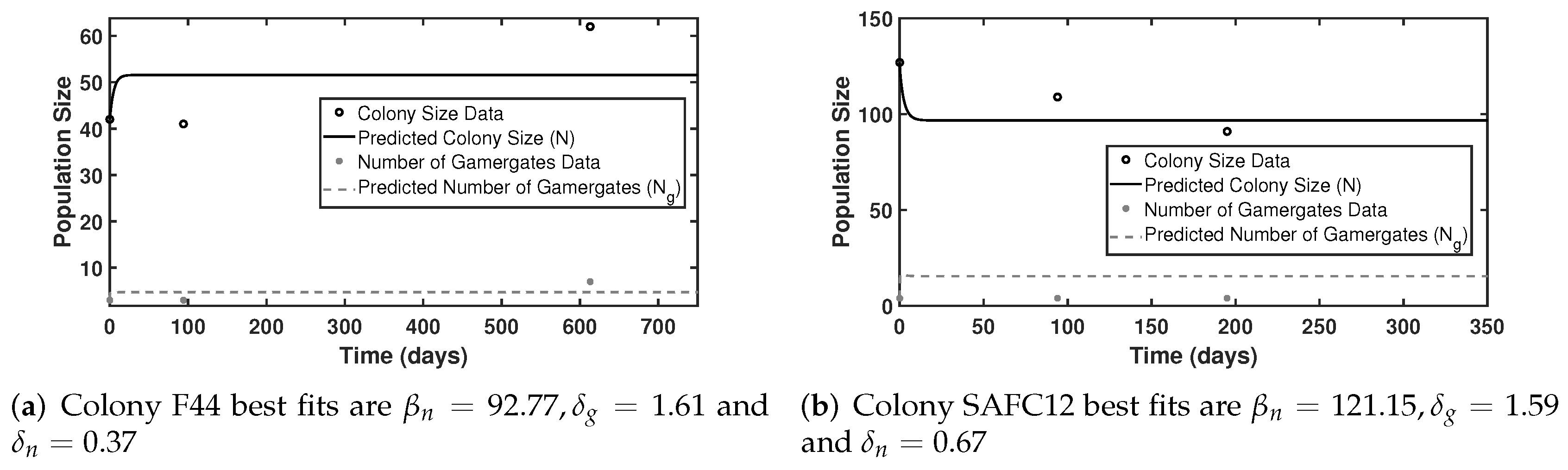
F44	0	42	3	0.0714
	94	41	3	0.0732
	613	62	7	0.1129
SAFC12	0	127	4	0.0315
	94	109	4	0.0360
	125	91	4	0.0440

), we fix $e=2.42$, $d_g=0.00028$, $d_w=0.0025$, and ${\beta }_g=33$ and estimate the values of ${\beta }_n$ and ${\delta }_i,i=n,g$ for each colony. The results are shown in

Table 3. Best fitting parameters (${\beta }_n,{\delta }_g,{\delta }_n$) of model (9) and (10) for colonies F44 and SAFC12. The fixed parameters are $e=2.42$, $d_g=0.00028$, $d_w=0.0025$, and ${\beta }_g=33$. Moreover, the colony size at equilibrium ($N^{*}$), number of gamergates at equilibrium ($N{g}^{*}$), and fraction of gamergates at equilibrium ($X^{*}$) for each colony are presented.

Colony	${\mathit{\beta }}_{\mathit{n}}$	${\mathit{\delta }}_{\mathit{g}}$	${\mathit{\delta }}_{\mathit{n}}$	${\mathit{N}}^{*}$	${\mathit{Ng}}^{*}$	${\mathit{X}}^{*}$
F44	92.77	1.61	0.37	51	5	0.098
SAFC12	121.15	1.59	0.67	97	15	0.155

. In Figure 4a, the fitted parameters for Colony F44 are ${\beta }_n=92.77,{\delta }_g=1.61$, and ${\delta }_n=0.37$ with the colony reaching a size of $N^{*}=51$, number of gamergates $N_g^{*}=5$, and the reproductive ratio $X^{*}=0.098$. In Figure 4b, Colony SAFC12 best fits are ${\beta }_n=121.15,{\delta }_g=1.59$, and ${\delta }_n=0.67$ which reaches a size of $N^{*}=97$, number of gamergates $N_g^{*}=15$, and reproductive ratio $X^{*}=0.155$. Our estimations seem to be in agreement with values of parameters presented in literature, and the predictions from our model are reasonable.

4.2. Simulations and Bifurcations

Our simulations suggest that the system (9) and (10) always has a unique interior equilibrium $(N^{*},N_g^{*})$ which appears to be globally stable, i.e., the colony would reach its stable reproductive ratio for a fixed set of parameter values. Observations from Figure 3 indicate that the metabolic parameters are crucial for the colony size N and the reproductive ratio X. The interior equilibrium $(N^{*},X^{*})$ depends on the metabolic parameters: Figure 3a,c shows that the larger the normalization measure of the gamergates ${\beta }_g$ and the hypometric relation factor of gamergates ${\delta }_g$, the smaller the colony size N and the reproductive ratio X. Figure 3b,d shows that the larger the normalization measure of the workers ${\beta }_g$ and the hypometric relation factor of workers ${\delta }_n$, the larger the colony size N and the reproductive ratio X. Figure 3 suggests that metabolic parameters of workers have opposite effects of gamergates’ metabolic parameters. To have a better picture of how ${\beta }_i$ and ${\delta }_i$ impact the colony size $N^{*}$ and the related reproductive ratio $X^{*}=\frac{N_g^{*}}{N^{*}}$, we highlight the curve of $N=\varphi \left(X\right)$ in red when $e=2.42$, $d_g=0.00028$, $d_w=0.0025$, ${\beta }_g=33$, ${\beta }_n=76.4$, ${\delta }_g=0.99,$ and ${\delta }_n=0.261$ which is the best approximation shown in Table 1. Four subfigures in Figure 3 suggest that the hypometric relation factor of metabolic rate ${\delta }_i$ is more sensitive than the normalization measure of ${\beta }_i$.

The bifurcation diagrams shown in Figure 5 were implemented to determine the effects of parameters, such as mortality and the egg laying rate, in shaping the hierarchy structure and demographics of the colony, i.e., N and X, respectively. In Figure 5a, as the parameter $d_g$ is increased in the range $(0.001;1)$ while fixing $e=2.42$, $d_w=0.0025$, ${\beta }_g=33$, ${\beta }_n=74.6$, ${\delta }_g=0.99,$ and ${\delta }_n=0.261$, the colony size $N^{*}$ decreases and the reproductive ratio $X^{*}$ increases. Similarly, as the parameter $d_w$ increases in the range $(0.0025;1)$ while fixing $e=2.42$, $d_g=0.00028$, ${\beta }_g=33$, ${\beta }_n=74.6$, ${\delta }_g=0.99,$ and ${\delta }_n=0.261$ (Figure 5b), the colony size $N^{*}$ decreases and the reproductive ratio $X^{*}$ increases. In Figure 5c, as the parameter ${\beta }_g$ increases in the range $(20;50)$ while fixing $e=2.42$, $d_g=0.00028$, $d_w=0.0025$, ${\beta }_n=74.6$, ${\delta }_g=0.99,$ and ${\delta }_n=0.261$, both the colony size $N^{*}$ and the reproductive ratio $X^{*}$ decrease. In contrast, in Figure 5d, as the parameter ${\beta }_n$ increases across the range $(35;150)$ while fixing $e=2.42$, $d_g=0.00028$, $d_w=0.0025$, ${\beta }_g=33$, ${\delta }_g=0.99,$ and ${\delta }_n=0.261$, both the colony size $N^{*}$ and the reproductive ratio $X^{*}$ increase. In Figure 5e, as the hypometric relation factor in gamergates (${\delta }_g$) increases across the range $(0;0.5)$ while fixing $e=2.42$, $d_g=0.00028$, $d_w=0.0025$, ${\beta }_g=33$, ${\beta }_n=74.6,$ and ${\delta }_n=0.261$, the colony size $N^{*}$ and the reproductive ratio $X^{*}$ decrease. In Figure 5f, as the hypometric relation factor in non-reproductive workers (${\delta }_n$) increases from 0 to $0.5$ while fixing $e=2.42$, $d_g=0.00028$, $d_w=0.0025$, ${\beta }_g=33$, ${\beta }_n=74.6,$ and ${\delta }_g=0.99$, the colony size $N^{*}$ and the reproductive ratio $X^{*}$ increase.

5. Conclusions

Complex hierarchies are prevailing in societies of both vertebrate and invertebrate species. In social insect colonies, the distribution of reproduction among the population in the colony can form linear, despotic, and nonlinear hierarchies. For example, the queenless colonies of the Ponerine ant, Harpegnathos saltator, have a shared (i.e., nonlinear) hierarchy [7]. Workers of H. Saltator establish a shared hierarchy for reproductive rights. Unlike most ant species, workers of H. Saltator retain the ability to mate and reproduce. Workers initiate a tournament after the death of their queen or when her fertility wanes to establish a subgroup of equally ranked reproductive individuals termed “gamergates” [13,40,41]. During tournaments, workers display three distinct agonistic interactions: dominance biting, physical policing, and antennal dueling, which are needed to form nonlinear shared hierarchies [7,32]. We have developed a compartmental model with nonlinear differential equations to address how the shared hierarchy depends on metabolic rates and life-history parameters related to colony size.

Our theoretical results presented in Theorem 2 provide insight into how mortality rates and metabolic parameters of gamergates and workers shape the nonlinear relationship between colony size (N) and the reproductive ratio (X). Under the conditions that the colony has ad libitum food, the mortality of gamergates is lower than that of non-reproductive workers, and that the metabolic rate of gamergates is higher than that of non-reproductive workers, our model predicts that the colony has a unique and stable interior equilibrium $(N^{*},N_g^{*})$ with $N_g^{*}$ being an increasing function of its reproductive ratio $X^{*}=\frac{N_g^{*}}{N^{*}}$. This prediction is in line with available biological data [38,39] (see Figure 2 and Figure 4).

Our model is able to use limited data to perform parameter estimations on the metabolic rate related parameters, ${\beta }_i,i=n,g$ and ${\delta }_i,i=n,g$, which is in the forms of ${\beta }_n{N}_n^{\delta }$ and ${\beta }_g{\left(XN\right)}_g^{\delta }$. By using laboratory data from 65 colonies and the ontological data of two individual colonies in the lab, our model provides some baseline ideas on the values of ${\beta }_i,i=n,g$, and ${\delta }_i,i=n,g$. Figure 3 suggests that the metabolic parameters are crucial for the colony size N and the reproductive ratio X. More specifically, the larger the values of the normalized metabolic rate of gamergates ${\beta }_g$ and the hypometric relation factor of gamergates ${\delta }_g$, the smaller the colony size N and the reproductive ratio X; meanwhile, the larger the values of the normalization measure of the workers ${\beta }_n$ and the hypometric relation factor of workers ${\delta }_n$, the larger the colony size N and the reproductive ratio X. It seems that the metabolic parameters of workers have an opposite effect than those of the gamergates. The additional bifurcation diagrams shown in Figure 5c–f confirm these observations and suggest that the hypometric relation factor of metabolic rate ${\delta }_i$ is more sensitive than the normalization measure ${\beta }_i$.

The bifurcation diagrams based on the mortality rate of workers $d_w$ (see Figure 5b) and the mortality rate of gamergates $d_g$ (see Figure 5a) show that increasing mortality leads to decreased colony size N and an increased reproductive ratio X. This result implies that a higher mortality rate would require higher investments in reproduction to sustain the population. Larger values of the metabolic parameters of non-reproductive workers (${\beta }_n,{\delta }_n$) result in larger colony size N and reproductive ratio X (see Figure 5d,f). This implies that the task performance of workers contributes to the colony’s function, and therefore, more investments in workers would benefit the colony. On the other hand, larger values of the metabolic parameters of gamergates (${\beta }_g,{\delta }_g$) result in smaller colony size N and reproductive ratio X (see Figure 5c,e). This indicates that the energy required for gamergates to maintain their reproductive status may negatively impact the size of their colony or the number of other gamergates that can be maintained.

The theoretic and bifurcation analysis of our model, validated by lab data, provides us important insights in addressing how may the key life-history parameters determine the colony demographic components $N,N_g,N_w$ and how the metabolic parameters affect the colony size, N, and shape the reproductive hierarchy $N_g$. It would be important to see how energetically demanding behaviors such as dominance biting, physical policing, and antennal dueling contribute to the stability of the hierarchy. Stochasticity should be included in future modeling efforts.

References

- Fewell, J.H.; Harrison, J.F. Scaling of work and energy use in social insect colonies. Behav. Ecol. Sociobiol. 2016, 70, 1047–1061. [Google Scholar] [CrossRef]
- Sidanius, J.; Pratto, F. Social Dominance: An Intergroup Theory of Social Hierarchy and Oppression; Cambridge University Press: Cambridge, UK, 1999. [Google Scholar] [CrossRef]
- Chase, I.D.; Tovey, C.; Spangler-Martin, D.; Manfredonia, M. Individual differences versus social dynamics in the formation of animal dominance hierarchies. Proc. Natl. Acad. Sci. USA 2002, 99, 5744–5749. [Google Scholar] [CrossRef] [Green Version]
- Broom, M. A unified model of dominance hierarchy formation and maintenance. J. Theor. Biol. 2002, 219, 63–72. [Google Scholar] [CrossRef]
- Hickey, J.; Davidsen, J. Self-organization and time-stability of social hierarchies. PLoS ONE 2019, 14, e0211403. [Google Scholar] [CrossRef] [Green Version]
- Chase, I.D.; Seitz, K. Self-Structuring Properties of Dominance Hierarchies: A New Perspective. Adv. Genet. 2011, 75, 51. [Google Scholar]
- Sasaki, T.; Penick, C.A.; Shaffer, Z.; Haight, K.L.; Pratt, S.C.; Liebig, J.; van Doorn, G.S.; Bronstein, J.L. A Simple Behavioral Model Predicts the Emergence of Complex Animal Hierarchies. Am. Nat. 2016, 187, 765–775. [Google Scholar] [CrossRef] [Green Version]
- Uhrich, J. The social hierarchy in albino mice. J. Comp. Psychol. 1938, 25, 373–413. [Google Scholar] [CrossRef]
- Kinsey, K.P. Social behaviour in confined populations of the Allegheny woodrat, Neotoma floridana magister. Anim. Behav. 1976, 24, 181–187. [Google Scholar] [CrossRef]
- Deslippe, R.J.; M’Closkey, R.T.; Dajczak, S.P.; Szpak, C.P. A quantitative study of the social behavior of tree lizards, Urosaurus ornatus. J. Herpetol. 1990, 24, 337–341. [Google Scholar] [CrossRef]
- Harcourt, A.H.; De Waal, F.B.M. (Eds.) Coalitions and Alliances in Humans and Other Animals; Oxford University Press: Oxford, UK, 1992. [Google Scholar]
- Reeve, H.K.; Keller, L. Tests of reproductive-skew models in social insects. Annu. Rev. Entomol. 2001, 46, 347–385. [Google Scholar] [CrossRef] [Green Version]
- Peeters, C.; Hölldobler, B. Reproductive cooperation between queens and their mated workers: The complex life history of an ant with a valuable nest. Proc. Natl. Acad. Sci. USA 1995, 92, 10977–10979. [Google Scholar] [CrossRef] [Green Version]
- Peelers, C.; Crozier, R.H. Caste and reproduction in ants: Not all mated egg-layers are “queens”. Psyche 1988, 95, 283–288. [Google Scholar] [CrossRef] [Green Version]
- Monnin, T.; Ratnieks, F.L. Reproduction versus work in queenless ants: When to join a hierarchy of hopeful reproductives? Behav. Ecol. Sociobiol. 1999, 46, 413–422. [Google Scholar] [CrossRef]
- Cant, M.A.; Field, J. Helping effort in a dominance hierarchy. Behav. Ecol. 2005, 16, 708–715. [Google Scholar] [CrossRef]
- Broom, M.; Cannings, C. Modelling dominance hierarchy formation as a multi-player game. J. Theor. Biol. 2002, 219, 397–413. [Google Scholar] [CrossRef]
- Beaugrand, J.P. Relative importance of initial individual differences, agonistic experience, and assessment accuracy during hierarchy formation: A simulation study. Behav. Process. 1997, 41, 177–192. [Google Scholar] [CrossRef]
- Jaffe, K. Quantifying social synergy in insect and human societies. Behav. Ecol. Sociobiol. 2010, 64, 1721–1724. [Google Scholar] [CrossRef]
- Waters, J.S.; Holbrook, C.T.; Fewell, J.H.; Harrison, J.F. Allometric scaling of metabolism, growth, and activity in whole colonies of the seed-harvester ant Pogonomyrmex californicus. Am. Nat. 2010, 176, 501–510. [Google Scholar] [CrossRef]
- Shik, J.Z.; Hou, C.; Kay, A.; Kaspari, M.; Gillooly, J.F. Towards a general life-history model of the superorganism: Predicting the survival, growth and reproduction of ant societies. Biol. Lett. 2012, 8, 1059–1062. [Google Scholar] [CrossRef]
- Dial, K.P.; Greene, E.; Irschick, D.J. Allometry of behavior. Trends Ecol. Evol. 2008, 23, 394–401. [Google Scholar] [CrossRef]
- Shik, J. Ant colony size and the scaling of reproductive effort. Funct. Ecol. 2008, 22, 674–681. [Google Scholar] [CrossRef]
- Cao, T.; Dornhaus, A. Larger laboratory colonies consume proportionally less energy and have lower per capita brood production in Temnothorax ants. Insectes Sociaux 2013, 60, 1–5. [Google Scholar] [CrossRef]
- Cole, B.; Wiernasz, D. Colony size and reproduction in the western harvester ant, Pogonomyrmex occidentalis. Insectes Sociaux 2000, 47, 249–255. [Google Scholar] [CrossRef]
- Penick, C.A.; Prager, S.S.; Liebig, J. Juvenile hormone induces queen development in late-stage larvae of the ant Harpegnathos saltator. J. Insect Physiol. 2012, 58, 1643–1649. [Google Scholar] [CrossRef]
- Ghaninia, M.; Haight, K.; Berger, S.L.; Reinberg, D.; Zwiebel, L.J.; Ray, A.; Liebig, J. Chemosensory sensitivity reflects reproductive status in the ant Harpegnathos saltator. Sci. Rep. 2017, 7, 3732. [Google Scholar] [CrossRef]
- Peeters, C.; Liebig, J.; Hölldobler, B. Sexual reproduction by both queens and workers in the ponerine ant Harpegnathos saltator. Insectes Sociaux 2000, 47, 325–332. [Google Scholar] [CrossRef]
- Liebig, J.; Poethke, H.J. Queen lifespan and colony longevity in the ant Harpegnathos saltator. Ecol. Entomol. 2004, 29, 203–207. [Google Scholar] [CrossRef]
- Mayoral, A. Analysis of Egg-Laying Rates of Harpegnathos saltator through Different Methods of Observation. Ph.D. Thesis, Arizona State University, Tempe, AZ, USA, 2017. [Google Scholar]
- Penick, C.A.; Ghaninia, M.; Haight, K.L.; Opachaloemphan, C.; Yan, H.; Reinberg, D.; Liebig, J. Reversible plasticity in brain size, behaviour and physiology characterizes caste transitions in a socially flexible ant (Harpegnathos saltator). Proc. R. Soc. B 2021, 288, 20210141. [Google Scholar] [CrossRef]
- Liebig, J. Eusociality, Female Caste Specialization, and Regulation of Reproduction in the Ponerine ant Harpegnathos Saltator Jerdon; Wiss.-und-Technik: Berlin, Germany, 1998. [Google Scholar]
- Liebig, J.; Hölldobler, B.; Peeters, C. Are ant workers capable of colony foundation? Naturwissenschaften 1998, 85, 133–135. [Google Scholar] [CrossRef]
- Waters, J.S.; Ochs, A.; Fewell, J.H.; Harrison, J.F. Differentiating causality and correlation in allometric scaling: Ant colony size drives metabolic hypometry. Proc. Biol. Sci. 2017, 284, 20162582. [Google Scholar] [CrossRef] [Green Version]
- Chown, S.; Marais, E.; Terblanche, J.; Klok, C.; Lighton, J.; Blackburn, T. Scaling of insect metabolic rate is inconsistent with the nutrient supply network model. Funct. Ecol. 2007, 21, 282–290. [Google Scholar] [CrossRef]
- Bourke, A.F. Worker reproduction in the higher eusocial Hymenoptera. Q. Rev. Biol. 1988, 63, 291–311. [Google Scholar]
- Franks, N.R.; Ireland, B.; Bourke, A.F. Conflicts, social economics and life history strategies in ants. Behav. Ecol. Sociobiol. 1990, 27, 175–181. [Google Scholar] [CrossRef]
- Stephens, D.W.; Krebs, J.R. Foraging Theory; Princeton University Press: Princeton, NJ, USA, 1986. [Google Scholar]
- Poethke, H.J.; Liebig, J. Risk-sensitive foraging and the evolution of cooperative breeding and reproductive skew. BMC Ecol. 2008, 8, 2. [Google Scholar] [CrossRef] [Green Version]
- Liebig, J.; Peeters, C.; Hölldobler, B. Worker policing limits the number of reproductives in a ponerine ant. Proc. R. Soc. Lond. Biol. Sci. 1999, 266, 1865–1870. [Google Scholar] [CrossRef]
- Hölldobler, B.; Wilson, E.O. The Superorganism: The Beauty, Elegance, and Strangeness of Insect Societies; WW Norton & Company: New York, NY, USA, 2009. [Google Scholar]