An Improved Point Clouds Model for Displacement Assessment of Slope Surface by Combining TLS and UAV Photogrammetry

Abstract

TLS can quickly and accurately capture object surface coordinates. However, TLS point clouds cannot cover the entire surface of the target object, due to block of view and limitation of measurement condition. Thus, using it to monitor deformation of slope reduces the detection accuracy of slope surface deformation. To overcome the drawbacks, a method to improve TLS point clouds by UAV photogrammetric point clouds is proposed. The two kinds of point clouds are registered as the new multi-view point clouds by PCA and ICP. The locations of monitoring points are extracted based on HSL color space recognition method from the new multi-view point clouds to analyze the surface displacement. At present, the proposed method has applied in a highway slope in Yunnan Province, and complete point clouds were successfully constructed. A RTK survey was used to compare and verify the proposed method. The verification result demonstrate that the difference of displacement between two measurement methods is less than 10 mm. Comprehensive experiments demonstrate that the proposed method is reliable and meets the slope displacement monitoring standard.

1. Introduction

The deformation of highway high slope usually causes the slope instability, which will lead to the occurrence of landslide and great harm to human society. Thousands of landslides have been reported annually, all over the world, and the number has extremely increased in recent years [1,2]. At present, highway high slopes are widely distributed, and the instability of highway slope brings great loss to human society [3]. Therefore, it has attracted the attention of governments, as well as experts and researchers in related fields worldwide.

Common slope stability monitoring methods, in project application, include laser scanner measurement, RTK positioning technology and UAV point clouds measurement [4,5,6]. At present, the more conventional slope deformation measurement method is the topographic survey carried out by Total Station and GNSS devices, as data acquisition sources of slope displacement. The accuracy of these methods, meet the accuracy requirements of slope measurement. However, there are many problems in the process of slope measurement, such as large amounts of tasks and vulnerable monitoring equipment a potential danger to the life of the surveyors during the steep slope operation.

In recent years, experts and researchers in related fields began to turn to image detection analysis for slope instability in pursuit of efficient and safe analysis methods. The image detection of slope damages such as surface crack, local collapse has been applied to slope instability analysis by UAV On-Site Inspection that is an image detection method [7,8]. However, it only identifies local slope damages. Thus, remote sensing-based techniques were proposed, including laser scanning point clouds, UAV photogrammetric point clouds, which can intuitive express the deformation of whole slope. Laser scanning is a widely used technology in a variety of fields especially in engineering. It mainly consists of three common types of laser scanning: ALS, TLS and MLS. ALS is mainly installed on the fixed wing aircraft or helicopter and can currently be fixed on a UAV, which has high scanning efficiency and flexible operation, but its measurement accuracy is lower. TLS is fixed scanning with high accuracy and long scanning range, but its scanning efficiency is lower. MLS is installed on the vehicle and has the characteristics of mobile scanning and high efficiency, but its measurement accuracy is lower. According to their own characteristics, ALS is more frequently used to estimate forest resources distribution survey [9], while TLS and MLS are usually used for engineering displacement analysis and deformation monitoring. In current research, the movement on surface and the displacement of landslide are studied [10] to prevent occurrences of hazard and risk by using TLS. Rock slope has also attracted extensive attention. The rockslide has been studied and some addressed approaches of using laser scanning were proposed to analyze the structure of steep scarp of rockslide and monitoring the failure position of large displacement of rock mass [11].

In a nutshell, TLS is usually used as a common monitoring and surveying approaches that has applied to a lot of research projects. However, in the actual field application, the data acquired by TLS often omits some level parts of slope surface because some level parts of slope surface cannot be captured by TLS. For instance, when the position of instrument is 25 m far from the toe of a 50 m high slope (consists of 4 horizontal platform), the TLS instrument cannot reach lowest platform to generate point clouds on it.

Targeting the disadvantages of TLS, ALS was used to provide missing point clouds from the overlook view and register with TLS. ALS usually generate 1–8 points per square meter and more points can be found in overlapping area [12]. However, it requires a high skill level of operators and the point densities of ALS are too sparse to fit displacement monitoring [13,14]. Studies on slope displacement measurement based on UAV photogrammetric point clouds have been carried out for some researches. An analytical method was explored that concluded a geometrical relationship among camera, measurement points and photographed images which made it possible to monitor the slope displacement by analyzing UAV photogrammetric point clouds [15]. The binocular vision system was used in the displacement monitoring for slope stability evaluation, which is convenient and accurate [16]. These studies supply a possibility for using UAV photography to analyze the slope displacement.

On UAV photogrammetric measuring, a way of image recognition [17] based on texture and tested one hundred UAV images to validate the correct classification rate was proposed. Based on the correct classification, the reliability of UAV for landslide body imaging detection and displacement analysis was proved by collecting real local landslide statistics [18]. Lucieer A et al. used UAV to collect images for many times, generated digital elevation model and analyzed the surface of two landslides at a certain time interval to calculate the displacement of landslide in that time period [19]. Besides, Yoon H et al. used UAV collecting video data and analyzed every picture to measure the civil infrastructure displacement such as bridges [20]. All the research provides a way of monitoring displacement by UAV images, however, the distortion was caused by camera lens that affect the accuracy of displacement analysis. It is of necessity to correct distortion before using the UAV images to work on a better accuracy level. However, due to the limitation of camera resolution and flight height, this method still cannot meet the requirements of slope displacement measurement accuracy.

At present, the scholars abroad and at home mostly focus on proposing new registration method and improving the registration efficiency. On the method proposition, Besl J forwarded a method of registration for 3D shapes [21] including point sets, curves and surfaces, it built the fundamental in registration field. Furthermore, fully automatic registration of 3D point clouds is proposed which includes coarse alignment based on extended Gaussian image and fine alignment based on ICP algorithm [22]. Based on the existing research, the image-based registration method for point clouds was also proposed. Zhu et al. proposed registration method using UAV images and LiDAR data generating 3D model [23]. Currently, Yun et al. concluded a new automated registration method by using sphere target to combine multi-view point clouds and developed a system to automatize the processing flow [24]. The time consumption of registration is also vital for ensuring the efficiency. Gressin put forward an improvement [25] for two steps of ICP [26] with optimal neighborhood knowledge and successfully applied it in ALS, TLS and MLS. Yan et al. proposed an algorithm combining genetic algorithm with ICP, which registers the TLS and MLS, and improved the efficiency of traditional GA registration method [27]. To solve the problem of high time consumption, a new point clouds automatic registration algorithm based on PCA algorithm and ICP algorithm is proposed [28]. There are adequate basic researches on point clouds registration, but most of them were concentrated on two entire point clouds registration which may consume much more time, so generating partial point clouds as complement to make up the view-blocked area is a more efficient way that proposed in this paper.

Generating point clouds by using UAV has some advantages that includes easy-operation, low hardware-cost and dense point clouds compare with generation cloud points by ALS [29], and can increase the point clouds density then improves accuracy in a certain way.

In this study, an improved point clouds model for displacement assessment of slope surface by combining TLS and UAV photogrammetry was used for the first time to calculate high slope surface displacement at a highway high slope in Yunnan Province. Entire structure of the paper is shown as follow: in Section 2, demonstrates the proposed method procedure of improving TLS point clouds. Several experiments to validate the accuracy improvement are carried out and on-site registered datum are collected, comparison between proposed method and traditional measurement method to test robustness in construction project is made in Section 3 as well. Section 4 draws some conclusions and listed some still existing issues need to be further learnt in the future.

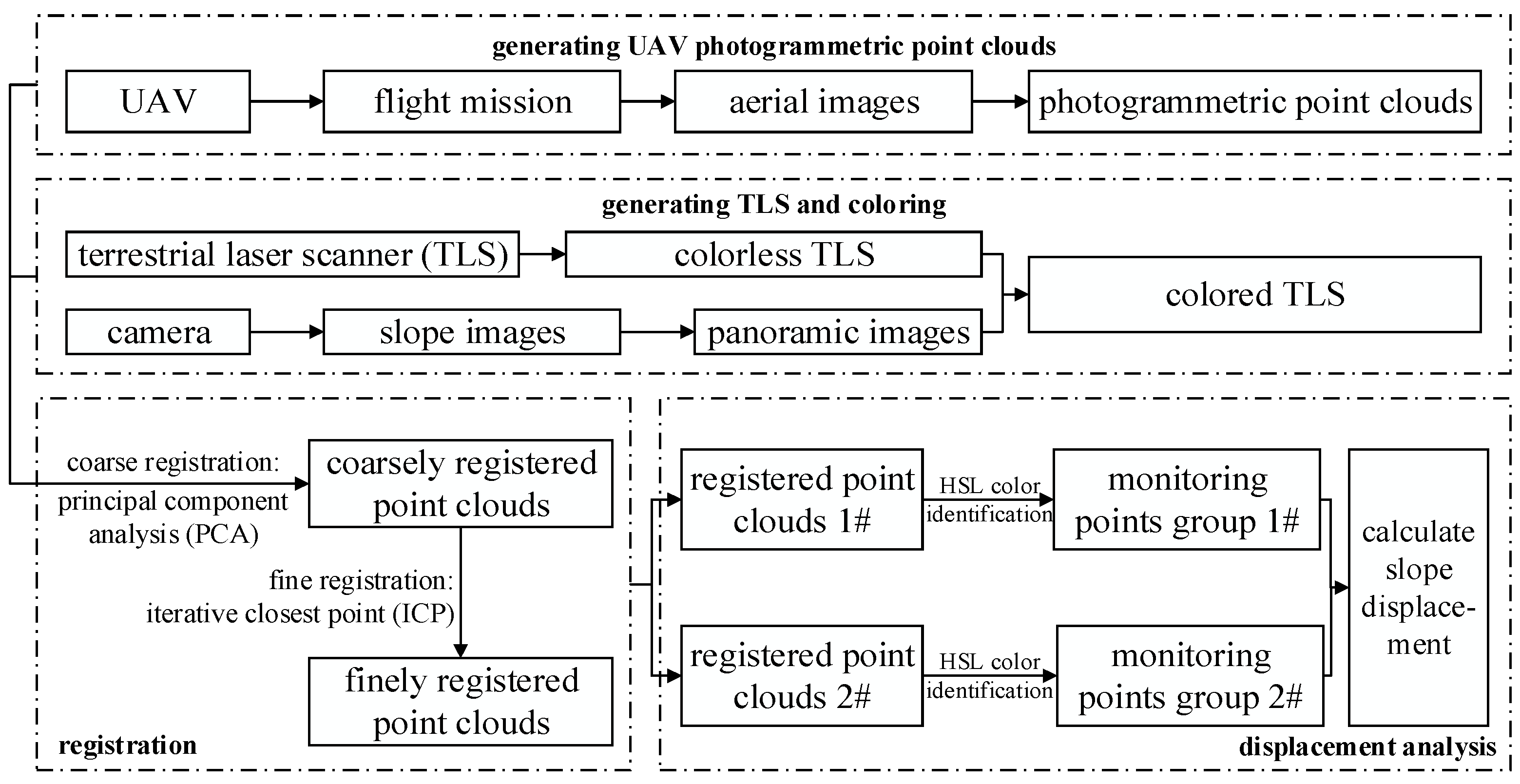
2. Methodology

The proposed method of improving TLS to monitoring surface displacement is compose of four parts: generating UAV photogrammetric point clouds, generating TLS and coloring, registration and displacement analysis. Based on the current studies and researches, a method to improve laser scanning point clouds by UAV photography on slope surface displacement analysis is proposed in this paper. The comprehensive processing flow is shown in Figure 1.

2.1. Generating UAV Photogrammetric Point Clouds

UAV photography point clouds reconstruction includes the following steps: UAV acquisition of images, image preprocessing, distortion correction, interest point recognition and matching, spatial conversion, sparse point cloud and point cloud encryption. The shoot process of UAV, the directional overlap rate is set to 85% and lateral overlap rate is set to 75%.

2.1.1. Image Preprocessing

In the process of exposure, imaging and recording, the image will be interfered and affected by certain factors such as mechanical movement and current generation, and there will be noise in the image that seriously affects the visual effect of the image, which reduces the image quality. Thus, the acquired images need to be processed by image filtering and image enhancement. Median filtering is used for image filtering, and histogram equalization is used for image enhancement. All optical camera lenses have the problem of distortion. Distortion is the geometric distortion of imaging, which is caused by the different magnification of the image in different areas on the focal plane. The degree of distortion increases from the center of the picture to the edge of the picture, and it is mainly reflected in the edge of the picture. The distortion problem is especially serious for remote photography [30], therefore, camera distortion of UAV needs to be corrected before generating UAV photogrammetric point clouds. Zhang’s camera calibration technique will be applied [31] as distortion correction method which has been widely adopted as a toolbox or packaged function in result of its high accuracy.

After distortion correction, interest points in UAV images needs to be distinguished and matched with algorithms such as SIFT and SURF, and a comparison between different algorithms was carried out. According to the result [32], the SIFT is more suitable for recognition and matching of points of interest. As shown in

Table 1. The comparison of SIFT and SURF algorithms.

No	1	2	3	4	5
Width × height/pixel	5472 × 3684		4608 × 3405
SIFT time-consuming/s	4.313	4.582	2.750	2.752	2.576
The number of feature points extracted by SIFT	426,067	448,317	13,796	29,538	9216
SURF time-consuming/s	3.915	4.833	1.734	1.910	1.517
The number of feature points extracted by SURF	139,640	127,072	4850	9156	3089

, interest points recognition of multiple groups of images were carried out in the study. It is found that SIFT usually takes more time, but more interest points are identified than SURF with better robustness. At the same time, SURF algorithm has some deficiencies in edge suppression, and more edge points are identified as interest points (Figure 2). In the process of UAV photography route planning, the robustness of size and rotation changes is required, and the matching accuracy is expected to be as high as possible. Finally, SIFT algorithm was adopted as the interest points identified algorithm.

2.1.2. Spatial Conversion

Before registration of two types of point clouds, the coordinate needs to be unified as world coordinate system due to UAV photographic measurement point clouds is generated in its own coordinate system. In a high-resolution image, every pixel, such as $P$($u,v$), is marked in image coordinate system. However, not all pixels have position associated mapping with the actual distance on the position, so the position coordinate system is introduced to bind pixel-position relationship and reflect the actual distance between any two pixels. For instance, there is a point in image which can be represented as ($x,y$) in the pixel position coordinate system, as Figure 3 shows. The interactive transforming relation can be presented as Equation (1). In the Equation (1), $\Delta x$ and $\Delta y$ are the unit distance on $x$-axis and $y$-axis between two adjacent pixels.

$$\left\{\begin{array}{c}u=\raisebox{1ex}{$x$}\!\left/ \!\raisebox{-1ex}{$\Delta x$}\right.+u_0\\ v=\raisebox{1ex}{$y$}\!\left/ \!\raisebox{-1ex}{$\Delta y$}\right.+v_0\end{array}\right. \mathrm{or}\left\{\begin{array}{c}x=\left(u-u_0\right)\Delta x\\ y=\left(v-v_0\right)\Delta y\end{array}\right.$$

(1)

Figure 4 then any pixel coordinate in camera coordinate system can be calculated as Equation (2). In the Equation (2), $z$ is the vertical distance from the camera to the origin of pixel position coordinate system.

$$\left\{\begin{array}{c}{x}_c=x=\left(u-u_0\right)\Delta x\\ y_c=y=\left(v-v_0\right)\Delta y\\ z_c=z_{O_c}+z=z_{O_c}+\left|O_c{O}_p\right|\end{array}\right.$$

(2)

The transformation from camera coordinate system to world coordinate system can be achieved by rotation matrix and translation matrix, presented as $\mathit{R}$ and $\mathit{T}$, respectively.

The camera on UAV automatically records the coordinate of it in world coordinate system, so the transformation can be executed itself. The final transformation relationship from image coordinate to pixel position coordinate to camera coordinate and finally to world coordinate system can be expressed as a series of equation matrix (Equations (3)–(5)).

$$\left[\begin{array}{c}u\\ v\\ 1\end{array}\right]=\left[\begin{array}{ccc}\raisebox{1ex}{$1$}\!\left/ \!\raisebox{-1ex}{$\Delta x$}\right.& 0& u_0\\ 0& \raisebox{1ex}{$1$}\!\left/ \!\raisebox{-1ex}{$\Delta y$}\right.& v_0\\ 0& 0& 1\end{array}\right]\left[\begin{array}{c}x\\ y\\ 1\end{array}\right]$$

(3)

$$z_c\left[\begin{array}{c}x\\ y\\ 1\end{array}\right]=\left[\begin{array}{ccc}\left|O_c{O}_p\right|& 0& \begin{array}{cc}0& 0\end{array}\\ 0& \left|O_c{O}_p\right|& \begin{array}{cc}0& 0\end{array}\\ 0& 0& \begin{array}{cc}1& 0\end{array}\end{array}\right]\left[\begin{array}{c}\begin{array}{c}{x}_c\\ y_c\end{array}\\ \begin{array}{c}{z}_c\\ 1\end{array}\end{array}\right]$$

(4)

$$\left[\begin{array}{c}\begin{array}{c}{x}_c\\ y_c\end{array}\\ \begin{array}{c}{z}_c\\ 1\end{array}\end{array}\right]=\left[\mathit{R}|\mathit{T}\right]\left[\begin{array}{c}\begin{array}{c}{x}_w\\ y_w\end{array}\\ \begin{array}{c}{z}_w\\ 1\end{array}\end{array}\right]$$

(5)

With the real coordinate of UAV photography, the actual distance and position relationship can be factually reflected, then the successive research work can go on.

2.1.3. Generating Encrypted Point Clouds

The generation of UAV photography point clouds starts from the matched interest points. First, the fundamental matrix (F) of the two images are calculated, then the Eigen matrix (E) is obtained through the relationship between the F and E, and then performs singular value decomposition (SVD) of E. The rotation matrix (R) and translation vector (T) of the camera between two images are calculated. The external parameters of the camera can be obtained by the above method. Combined with the internal parameters of the camera, both the internal and external parameters of the current image will be obtained. The position of pixels in the real space can be recovered by triangulation. Because the triangulation method sometimes has some errors in positioning, it is necessary to optimize positioning. After the interest points between the two images are spatially located, the above steps are recirculated to spatially locate the interest points in the subsequent images. When all the interest points in the images are restored to the three-dimensional space, the point cloud formed by the interest points in the current UAV image can be obtained. Figure 5 shows the generation process of UAV point clouds base on matching interest points.

The point clouds generated based on the matching interest points between images is sparse and exists many regional distribution points on the slope which greatly affected the accuracy of measurement. As the basic of UAV complementary photogrammetric point clouds, interest points are replaced into the space and densified by using patch-based multi-view stereo (Figure 6) [33]. PMVS is used to calibrate multi-view stereopsis. It outputs a set of dense rectangular patches that cover the surfaces visible in the input photogrammetric images. PMVS associates with each image $I_i$ a regular grid of w × w pixels cells $C_i\left(x,y\right)$ and tries to reconstruct at least one patch in every image. The algorithm consists of three procedure as follow:

(1)

Feature Matching: features discovery by Harris and Gaussians operators are first matched across input images, which yields a sparse set of patches associated with salient image regions;

(2)

Patch expansion: as the main part of the PMVS, output a dense set of patches by spreading the initial patches to around pixels;

(3)

Filtering: incorrect matches need to be eliminated by visibility constraints.

2.2. Generating TLS and Coloring

2.2.1. Laser Scanning Point Cloud Acquisition

The working principle of the TLS is similar to the traditional total station. TLS scan surrounding objects by transmitting a large number of laser beams at high speed, and calculating the distance, horizontal angle, and vertical angle of the corresponding position according to laser reflection. These parameter are stored in the formatted point clouds data. Taking the Trimble TX8 TLS as an example, it can obtain information of objects within the range of 340 m at the furthest in the scanning process with a field of view of 360° × 317° (Figure 7).

Table 2. Relationship between TX8 scanning accuracy level and acquired data.

Scanning Parameters		Precision Grade
		Preview the Scan	Accuracy Level 1	Accuracy Level 2	Accuracy Level 3	Expanded Scan
Maximum range		120 m	120 m	120 m	120 m	340 m
Scan time		1 min	2 min	3 min	10 min	20 min
The spacing of point clouds at different distances	10 m	15.1 mm	-	-	-	-
	30 m	-	22.6 mm	11.3 mm	5.7 mm	7.5 mm
	300 m	-	-	-	-	75.4 mm
The number of cloud point generated		8.7 × 105	3.4 × 106	1.38 × 108	5.55 × 108	3.12 × 108

shows the relationship between the main accuracy levels and the obtained data.

In the process of collecting TLS point clouds, it is necessary to pay attention to the location of the scanner and the site environment. TLS is an optical device, it is affected by perspective relationship. Therefore, when the slope is high, the lower slope may partly block the upper slope due to perspective relationship. The point clouds of this part can be supplemented by point cloud generated by UAV photography. In addition, if there is fog or dust on site, small particles scattered in the air will also affect the process of point clouds acquisition. Therefore, data collection should be carried out as far as possible under clear weather and good sight conditions.

Point clouds includes the measured object’s reflection intensity, the times of reflection and its x, y and z coordinates relative to the set position of the scanner. However, it does not include the corresponding color and texture information of the measured object. Scanned point clouds without RGB color cannot be used to calculate the slope surface displacement by the method of identifying the monitoring points based on the color. In addition, since point clouds coordinates generated by TLS are generated relative to the position set by scanner. Generated point clouds need to be converted to same coordinate system as point clouds generated by UAV for registration [34].

2.2.2. Point Clouds Coloring

Point clouds coloring for TLS requires matching point clouds with the color digital panoramic image. In this study, point clouds coloring is completed in software Trimble Realworks 10.0.1. The point cloud coloring of TLS is the fitting process of point cloud file and panorama file by RealColor of Trimble Realworks and the fitting process is divided into manual fitting and automatic fitting. The fitting effect of the manual fitting is better comparing with automatic fitting. Thus, the manual fitting is selected to complete Point clouds coloring by matching three key points. The Kolor Autopano Giga 3.7 is used to generate panorama image with the help of images captured with a digital camera.

A digital camera installed on a tripod will be used with a wide-angle lens. Because common lenses and wide-angle lenses used are different, wide-angle lenses needs to be calibrated that make point clouds and colorful panoramic image match well (Figure 8).

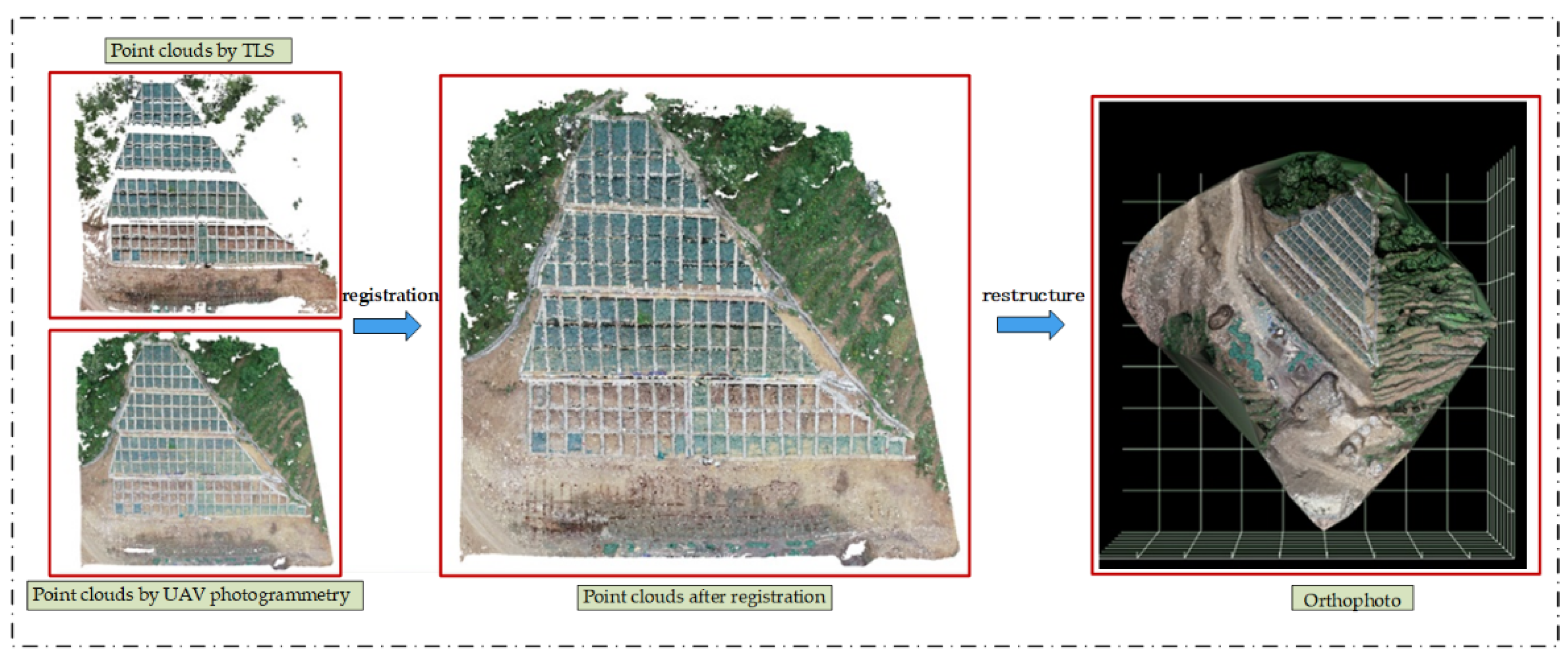
2.3. Registration

Point clouds registration is a process in which two groups of point cloud data with overlapping regions are aligned in the same coordinate system through coordinate transformation to form a complete point cloud data. The match points are some circular or square concrete piles and painted in vivid color which can be easily found and set near the view-blocked area where point clouds can be generated. A large number of complementary point clouds appeared at the edge of the point clouds loss region, and a large number of point clouds were generated in this region (Figure 9). Registration consists of two parts: coarse registration and fine registration.

2.3.1. Coarse Registration

Coarse registration is carried out with PCA. PCA is used to reduce the dimensionality of data. It retains some characteristics of large variance in point clouds, and is used to ensure that the coarse registration process reaches better efficiency and accuracy. Assuming two point sets: UAV photogrammetric point clouds as $\mathit{P}=\left\{p_1,p_2,p_3,\dots ,p_n\right\}$, TLS as $\mathit{Q}=\left\{q_1,q_2,q_3,\dots ,q_m\right\}$, calculate the centroid $\overline{p}$ (Equation (6)), $\overline{q}$ (Equation (7)) and covariance matrix $cov$ (Equation (8)).

$$\overline{p}=\raisebox{1ex}{$1$}\!\left/ \!\raisebox{-1ex}{$n$}\right.{{\displaystyle \sum }}_1^n{p}_i,\mathrm{as} \left[\begin{array}{c}\overline{x}\\ \overline{y}\\ \overline{z}\end{array}\right]=\raisebox{1ex}{$1$}\!\left/ \!\raisebox{-1ex}{$n$}\right.\left[\begin{array}{c}{{\displaystyle \sum }}_1^n{x}_i\\ {{\displaystyle \sum }}_1^n{y}_i\\ {{\displaystyle \sum }}_1^n{z}_i\end{array}\right]$$

(6)

$$\overline{q}=\raisebox{1ex}{$1$}\!\left/ \!\raisebox{-1ex}{$n$}\right.{{\displaystyle \sum }}_1^n{q}_i,\mathrm{as}\left[\begin{array}{c}\overline{x}\\ \overline{y}\\ \overline{z}\end{array}\right]=\raisebox{1ex}{$1$}\!\left/ \!\raisebox{-1ex}{$n$}\right.\left[\begin{array}{c}{{\displaystyle \sum }}_1^n{x}_i\\ {{\displaystyle \sum }}_1^n{y}_i\\ {{\displaystyle \sum }}_1^n{z}_i\end{array}\right]$$

(7)

$$cov=\left[\begin{array}{ccc}cov\left(x,x\right)& cov\left(x,y\right)& cov\left(x,z\right)\\ cov\left(y,x\right)& cov\left(y,y\right)& cov\left(y,z\right)\\ cov\left(z,x\right)& cov\left(z,y\right)& cov\left(z,z\right)\end{array}\right]$$

(8)

The eigenvalues and eigenvectors were calculated based on $cov$, and the original coordinates were redecomposed long the direction of the eigenvectors to obtain the UAV photogrammetric point clouds in the eigenvector coordinate system. Similarly, the centroid $\overline{q}$ of TLS point clouds is shifted to make it coincide with the centroid $\overline{p}$ of UAV photography point clouds, and TLS point clouds in the feature vector coordinate system are transformed to the direction of the UAV photography point clouds through rotation, so that the two coordinate systems are unified. At this time, point clouds of the two parts are converted to the same coordinate system and a preliminary registration of the overall fusion point clouds is obtained. Finally, the position of the two point clouds is judged by the point clouds minimum boundary box [35]. Minimum bounding box is an algorithm to solve the optimal enclosing space of discrete point sets. It replaces complex geometric objects with slightly larger volume and simple characteristics, as shown in Figure 10. Since the point clouds in the minimum enveloping box all meet the conditions:

$$\left\{\begin{array}{c}{x}_{min}\le x_c\le x_{max}\\ y_{min}\le y_c\le y_{max}\\ z_{min}\le z_c\le z_{max}\end{array}\right.$$

(9)

Therefore, each vertex ($(x_{max},y_{max},z_{max}$),$(x_{min},y_{max},z_{max}$), $(x_{max},y_{min},z_{max}$), $(x_{max},y_{max},z_{min}$), $(x_{min},y_{min},z_{max}$), $(x_{min},y_{max},z_{min}$), $(x_{max},y_{min},z_{min}$), $(x_{min},y_{min},z_{min}$)) of the minimum bounding box can be found by reading the maximum and minimum values of x, y and z in the point clouds, then, the region of the bounding box is delineated. Finally, the overlap rate of between the two point clouds bounding box can be used to judge whether the coordinate direction of the two part point clouds is opposite. When the overlap rate (The ratio of the number of point clouds in the overlapping region of the enveloping box to the total number of point clouds in itself) of the two point clouds exceeds a threshold, the coordinates of the two point clouds are in the same direction, and the coarse registration of the two part point clouds is completed. In this study, the overlap rate threshold was set at 90%.

2.3.2. Fine Registration

After coarse registration, the centroid coordinate of each point sets group will be calculated as the center of matching point to find the closest matched one in TLS point clouds. Then fine registration will be carried out. ICP is adopted as fine registration method, which is an algorithm for accurate registration of two point sets. ICP looks for points with a corresponding relationship between the two point sets and puts forward the points with a corresponding relationship to form a point set and regards the point set as a rigid body. After calculating the centroids of two rigid bodies, the centroid of two rigid bodies are rotated and shifted for making them close to each other. Then through iteration, the distance between the two point sets is gradually reduced and the direction tends to be the same. From a mathematical point of view. By repeatedly determining the corresponding point relation and calculating the rigid body transformation, two points are successfully matched when the distance between two point sets is less than a certain convergence threshold. ICP algorithm processing flow is shown in Figure 11.

Let P and Q be the corresponding point sets in the UAV photogrammetric point clouds and TLS point clouds, respectively. The main process of ICP algorithm includes the following steps:

(1)

Constructing the objective function of the least square method and setting the threshold as $\Delta$:

$$E\left(\mathit{R},\mathit{T}\right)=\frac{1}{n}{{\displaystyle \sum }}_{i=1}^n\Vert q_i-{\left(\mathit{R}{p}_i+\mathit{T}\right)\Vert }^2$$

(10)

where, the objective function $E$ is the mean of the sum of each distances between corresponding point pair, $p_i$ is in the point set $\mathit{P}$ and $q_i$ is in the point set $\mathit{Q}$, $\mathit{R}$ and $\mathit{T}$ are the rotation matrix and translation matrix respectively.

(2)

Find the centroid ${\mu }_p$ and ${\mu }_q$ of the point set $\mathit{P}$ and $\mathit{Q}$, and convert the position relation of each point into the relative centroid position relation:

$${\mu }_p=\frac{1}{n}{{\displaystyle \sum }}_{i=1}^n{p}_i$$

(11)

$${\mu }_q=\frac{1}{n}{{\displaystyle \sum }}_{i=1}^n{q}_i$$

(12)

$$p_i^{\prime }=p_i-{\mu }_p, q_i^{\prime }=q_i-{\mu }_q$$

(13)

(3)

The matrix $\mathit{M}$ is constructed according to ${\mathit{P}}^{\prime }$ and ${\mathit{Q}}^{\prime }$ obtained after transformation, so that:

$$\mathit{M}={{\displaystyle \sum }}_{i=1}^n{p}_i^{\prime }{q}_i^{\prime }{}^T$$

(14)

(4)

Singular value decomposition of matrix $\mathit{M}$ can be obtained:

$$\mathit{M}=\mathit{U}\mathit{\Sigma }{\mathit{V}}^T=\mathit{U}\left[\begin{array}{ccc}{\sigma }_1& 0& 0\\ 0& {\sigma }_2& 0\\ 0& 0& {\sigma }_3\end{array}\right]{\mathit{V}}^T$$

(15)

$$\mathit{D}=\left\{\begin{array}{c}{\mathit{I}}_3=\left[\begin{array}{ccc}1& 0& 0\\ 0& 1& 0\\ 0& 0& 1\end{array}\right] \det \left(\mathit{U}\right)\det \left(\mathit{V}\right)\ge 0\\ \mathit{d}\mathit{i}\mathit{a}\mathit{g}\left(1,1,-1\right)=\left[\begin{array}{ccc}1& 0& 0\\ 0& 1& 0\\ 0& 0& -1\end{array}\right] \det \left(\mathit{U}\right)\det \left(\mathit{V}\right) < 0\end{array}\right.$$

(16)

(5)

When $rank\left(\mathit{D}\right)$ ≥ 2, $\mathit{R}=\mathit{U}\mathit{D}{\mathit{V}}^T$:

$$\mathit{R}=\mathit{U}\mathit{D}{\mathit{V}}^T,\mathit{T}={\mu }_q-\mathit{R}{\mu }_p$$

(17)

When $rank\left(\mathit{M}\right)$= 3, there is a unique optimal rotation matrix ${\mathit{R}}_{\mathit{o}\mathit{p}\mathit{t}}$ and translation matrix ${\mathit{T}}_{\mathit{o}\mathit{p}\mathit{t}}$, making the objective function $E \left(\mathit{R},\mathit{T}\right)$ minimum.

$${\mathit{R}}_{\mathit{o}\mathit{p}\mathit{t}}=\mathit{U}{\mathit{V}}^T,{\mathit{T}}_{\mathit{o}\mathit{p}\mathit{t}}={\mu }_q-{\mathit{R}}_{\mathit{o}\mathit{p}\mathit{t}}{\mu }_p$$

(18)

(6)

Finally, the value of the objective function was calculated under the current rotation matrix and translation matrix, and be compared with the threshold. If the value is less than the threshold, the iteration ends; otherwise, the cycle is repeated step (2).

Point clouds after matching and registration are shown in Figure 11. Compared with the point clouds generated by UAV, the density of registration point clouds is well (Figure 12). The cloud points by TLS omit the horizontal part point clouds (Figure 12a). Both the matching and registration were completed and achieved by developed slope monitoring software which uses C++ as programming language and Qt as foreground interface. The development requirements of the slope monitoring system includes hardware device, software and development environment (

Table 3. The development requirements of the system.

	Tool Classification	Tool Name
Hardware device	UAV	DJI Matrice 600 Pro
	TLS	Trimble TX8
	Digital Camera	Canon 5D MarkIII
	Workstation	Dell PowerEdge R930
Software	Flight control software	DJI Go 4
		DJI GS Pro
	TLS data processing software	Trimble Realworks 10.0.1
	UAV point cloud generation software	Pix4D 4.4.12
Development environment	System development platform	Visual Studio 2015
	Programming language	Visual C++
	Front-end interface framework	Qt 5.7.0
	Image processing algorithm library	OpenCV, PCL
	Graphics processing and rendering visualization tools	Visualization Toolkit

). The system adopts C/S (Client/Server) architecture as the development mode. The open source OpenCV computer vision algorithm library is used to realize image processing and computer vision general algorithm. With the help of Bundler and PMVS, three-dimension reconstruction of structure from motion is realized. Using Visualization Toolkit (VTK) as a point cloud and reconstruction model rendering display tool, a set of multi-vision system for slope surface displacement is developed to achieve the function of obtaining high-precision point cloud, calculating slope surface displacement and slope stability analysis. Due to the limitation of the research range of this paper, details are not going to be demonstrated here, system functional framework as shown in Figure 13.

2.4. Color Space Selection

The displacement calculation is based on the two registration point clouds to find monitoring points with the same characteristics on the slope, monitoring points recognition through the color value, the initial data are expressed in RGB color space by numerical, but some disadvantages was found in the actual application, under the color space, monitoring points with the same characteristics will be under different light conditions present a different color value. For monitoring points in different time periods, RGB colors are different, and different RGB colors extracted inevitably complicates the identification process of monitoring points and affects the accuracy of identification.

Based on literature review, it is found that each color in HSL color space is represented by a unique set of indicators, namely, hue H, saturation S and brightness L. To verify the above view, the RGB color and HSL color of five monitoring points in two time periods are recorded through experiments (

Table 4. Comparison table of RGB color and HSL color of five monitoring points in two time periods.

Shooting Time	Monitoring Point Number	Monitoring Point Color
		R	G	B	H	S	L
10:30 a.m.	MP 1	232	131	145	352	0.44	0.91
	MP 2	237	138	152	352	0.42	0.93
	MP 3	237	130	152	348	0.45	0.93
	MP 4	235	134	151	350	0.43	0.92
	MP 5	240	132	144	353	0.45	0.94
3:53 p.m.	MP 1	199	101	118	350	0.49	0.78
	MP 2	209	109	125	350	0.48	0.82
	MP 3	192	111	119	354	0.42	0.75
	MP 4	191	113	126	350	0.41	0.75
	MP 5	201	113	126	351	0.44	0.79

). It can be seen from the Table 4 that light has a great influence on the color value of RGB space, light has a great influence on the L value of HSL color space, and little influence on H and S. Therefore, in this study, H and S were extracted to eliminate the interference of light on the extraction of monitoring points. The conversion relations are shown in Equations (19)–(21) [36]. The formula for converting RGB color space into HSL color space is as follows:

$$H=\left\{\begin{array}{c}\theta G\ge B\\ 2\pi -\theta G<B\end{array}\right.\mathrm{where}\theta ={\cos }^{-1}\left(\frac{2R-G-B}{2\sqrt{{\left(R-G\right)}^2+\left(R-B\right)\left(G-B\right)}}\right)$$

(19)

$$S=1-\frac{3 \min \left(R,G,B\right)}{R+G+B}$$

(20)

$$L=\frac{R+G+B}{3\times 255}$$

(21)

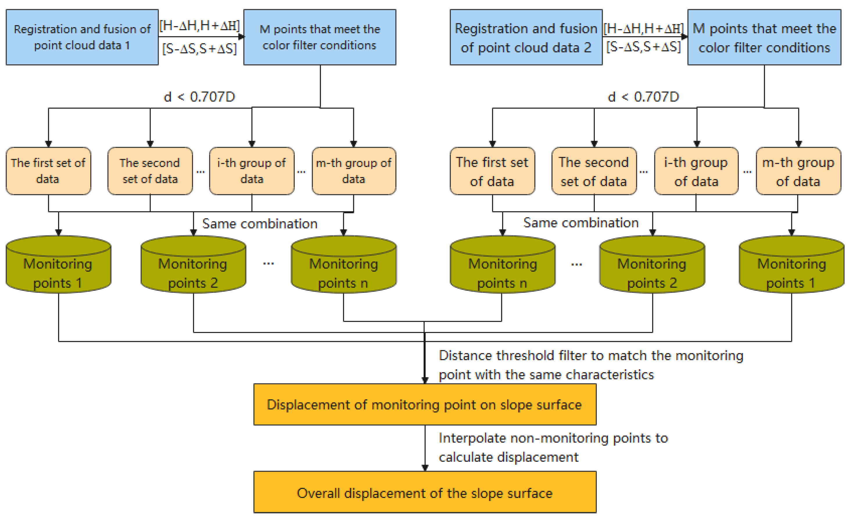
2.5. Displacement Calculation

The main idea of displacement calculation based on monitoring points is to set several monitoring points in advance on the slope to be measured, and find the monitoring points with the same characteristics in the results of two times reconstruction cloud points. Finally, calculating the coordinate difference based on the center point identified by two homonymous monitoring points, so as to obtain the displacement of this point on the slope.

Since the generated point clouds are disordered, it is the premise of displacement calculation to accurately distinguish and match the monitoring points with the same characteristics of two measured data from point clouds. In this study, all points in point clouds were searched by traversal. HSL space color was adopted as the recognition standard for the identification of the monitoring points. The monitoring points were extracted, and the displacement was calculated by matching between two times measurements. The main process is as follows (Figure 14):

(1)

Firstly, the recognition range of H and S parameters in the color of HSL space was determined according to the collected images and point clouds were screened to extract all points within the range of $\left[H-\Delta H,\hspace{0.17em}H+\Delta H\right]$, $\left[S-\Delta S,\hspace{0.17em}S+\Delta S\right]$ from point clouds;

(2)

The square side length of the monitoring point was named as D, and the distance d_ij between the ith point (0 < i ≤ m) and the jth point (0 < j ≤ m and j ≠ i) among the m points was calculated and screened out. If d_ij < 0.707 d ($d$, the distance from the center of the square monitoring point to the four corners), the jth point was divided into the ith group of data;

(3)

If there are points in group i + 1 that are the same characteristics as those in group i, the data in group i + 1 and group I are considered to represent the same monitoring point, and the two sets of data are combined to obtain n sets of data, where n should be equal to the number of monitoring points arranged;

(4)

Calculate N groups of data determined in the previous step to find the centroid of each group of data points, that is, the centroid is considered to be the center point within the painting range of the monitoring point, representing the position of the monitoring point;

(5)

According to the monitoring point was identified, the closest two points between the monitoring point in the second time registration point clouds and the monitoring points in the first time registration point clouds are regarded as the monitoring point with the same characteristics. Setting the distance threshold avoids matching the situation of the dislocation. When access to two of the coordinates of point clouds of monitoring points with the same characteristics, the calculation can be carried out according to the displacement calculation formula of the two-point coordinates.

3. Results

In this study, DJI Matrice 600 Pro, Canon 5D MarkIII and Trimble TX8 were used for data collection (Figure 15). The data acquisition of the system mainly includes three data acquisition of UAV image, TLS point cloud and color panoramic image. DJI Matric 600 Pro was used to collect aerial images. DJI GS Pro was used as route planning software to delimit UAV photography areas. Trimble TX8 TLS is installed 20 m away from the slope. The highest accuracy Level 3 is used to generate point clouds. After the scanning is completed, the position of TLS is changed to digital camera equipped with wide-angle lens to take a photo every 60°. A photo was taken vertically upward and downward, and six color photos were used for the generation of panoramic image mosaic (Figure 16). Color was provided to the point clouds by matching with the colorless point clouds of TLS by Trimble Realworks.

3.1. Experimental Area

The experimental area is located between Yunnan and Sichuan provinces, China. Relying on Zhaotong Expressway project, there are 26 high slopes in section A5 of Yiliang-Zhaotong section of Zhaotong expressway (Figure 17). The maximum height of slope excavation is 93.45 m, with 10 stages (k153 + 423 ~ k153 + 599 section); the minimum height of slope excavation is 27.4 m and the grade is 3 (k158 + 978 ~ k159 + 139 section). Mainly rock slope and composite slope.

In the early stage of construction, the stability of the high slope in the experimental area was analyzed, it is found that some slopes have poor stability. Therefore, the stability monitoring of the slope should be carried out to regularly grasp the current slope deformation, and timely reinforce the slope in case of large deformation, so as to prevent potential slope sliding, collapse, landslide and other accidents.

3.2. Accuracy and Flight Altitude Correlation

There is a conflict between the UAV resolution and image range. On the premise that camera parameters remain unchanged, the wider capture area, the fewer pixels are distributed over a certain area. Hence, the UAV flight altitude is an essential factor to the accuracy of displacement analysis and clarifying the correlation between accuracy and flight altitude helps to control the accuracy of this proposed method, meanwhile, further guarantee the validation of the result.

Several experiments were carried out in on-site researches. In the experiments, there were three factors taken into consideration, including flight altitude, monitoring point area and the measurement error comparing with actual displacement based on the T = total station or RTK survey. Because the shape of the monitoring points are always sets as square or circle, the side length or radius are used in analysis instead of the area.

In the field study, monitoring points and datum points need to be set up (Figure 18), red square were used as monitoring point and blue square were used as datum point. The datum point is used to calibrate coordinate system of point clouds by UAV and the coordinate of datum point was measured by a RTK survey. The calibrate process is carried out by marking datum point in every image. The monitoring point needs to be measured to obtain its own displacement. In the process of measurement, the monitoring point will be identified by set the value color H and S of HSL color space.

The flight heights of UAV were set at different elevations such as 20 m, 30 m, 40 m, 50 m, 60 m, 70 m, 80 m, 90 m, 100 m, 110 m and 120 m respectively. The side lengths of the selected monitoring points are 15 cm, 20 cm, 30 cm, 40 cm and 45 cm, respectively. Controlling the error within 10 mm, the correlation between flight altitude and monitoring point size is shown in Figure 19a, it is easy to conclude an approximate linear correlation that with the flight altitude rises, the size needs to be set larger. In Figure 19b, when controlling the flight altitude as a constant (30 m) to analyze the correlation between monitoring point size and error that draw a conclusion: the larger the size of the monitoring point, the smaller the error. When controlling the size of monitoring point (40 cm), the correlation of the UAV flight altitude and error is shown in Figure 19c.

It is exactly obvious that there are some results can be concluded as follow: (1) Approximate linear correlation between monitoring point size and UAV flight altitude can be presented as an equation $y=0.33x+9.24$. It shows that to make the error meet the requirements of construction project and specification, the monitoring point size needs to be set larger when the UAV altitude rising. (2) Monitoring point is better from 30 cm to 45 cm, accordingly the measurement error will be reduced with the size increases in a certain extent. (3) In order to ensure the validation of this method, when the size of monitoring point is set to 40 cm, it is recommended that the UVA altitude of less than 60 m. While the altitude excess 60 m, the measurement error will increase greatly and quickly. However, in the application, the relative height cannot be strictly controlled.

3.3. Comparison between Different Methods

This article uses three methods (only using UAV, only using TLS, and a combination of the two to form a registration point clouds). The comparison index includes horizontal error, inclined error and RMSE (Equation (22)). Horizontal error is the error between actual displacement and measure displacement of monitoring point on a horizontal plane. Inclined error is the error between actual displacement and measure displacement of monitoring point on an inclined plane.

The comparison results are shown in

Table 5. Comparison of the three methods in the number of monitoring points, horizontal error, inclined error and root mean square error.

Index	UAV	TLS	UAV + TLS
Number	10	7	10
Horizontal error	10 mm	-	-
Inclined error	20–30 mm	10 mm	-
RMSE	1.2 mm	0.48 mm	0.73 mm

. The horizontal error and inclined error is the absolute error between actual displacement and measure displacement.

$$RMSE=\sqrt{\frac{1}{m}{{\displaystyle \sum }}_{i=1}^m{(l_i-{\widehat{l}}_i)}^2}$$

(22)

where, $l_i$ is the measured value of ith monitoring point displacement, ${\widehat{l}}_i$ is the actual value of ith monitoring point displacement and m is the number of monitoring points.

When only using UAV for displacement measurement, the number of monitoring points identified is 10, which is more accurate when measuring the displacement of the monitoring points arranged on the horizontal plane and can be basically controlled within 10 mm, but when measuring the displacement of the monitoring points on the inclined plane, the direction error is relatively large, about 20–30 mm. The RMSE is 1.2 mm.

When only using TLS to measure the displacement of a slope surface, due to the limitation of the viewing angle, the horizontal monitoring points arranged on the step slope platform cannot be scanned. Finally, the number of monitoring points identified is 7, the displacement measurement accuracy of the 7 monitoring points on the inclined surface in all three directions (x, y and z) can be measured. The RMSE is 0.48 mm.

When using TLS and UAV to generate a registration point clouds for slope surface displacement measurement, the number of monitoring points identified is 10, the measurement accuracy can reach less than 10 mm and the RMSE is 0.73 mm. The displacement of 10 monitoring points are shown in Figure 20.

As shown in the Figure 20, the displacement accuracy of horizontal monitoring points higher the inclined monitoring points by UAV. The displacement curves measured by UAV + TLS are similar to the actual displacement curves and have a high degree of coincidence. The displacement accuracy measured of the inclined monitoring points by UAV + TLS is higher than by TLS alone. The error of horizontal monitoring displacement larger than the error of inclined monitoring displacement by UAV + TLS.

3.4. On-Site Practical Result

This paper relies on the slope of a highway construction project in Yunnan, China to verify the improved method of surface displacement monitoring on five large-scale slopes. The on-site practical experiments implemented DJI M600 Pro and Trimble TX8 TLS as the slope image and point clouds data acquisition devices. The TLS is erected at the point 28.2 m away from the slope toe line of the vertical slope.

Besides the monitoring points set on slope, there are some squares can be mobilized to manual stimulate large displacement situation. After data collection and UAV image distortion correction, the complement point clouds made up the block area which TLS view cannot reach. The registration of two point clouds formed a complete datasets, thus, the surface displacement was calculated. In order to improve the visual display, the orthophoto was generated based on the registered point cloud, as shown in the Figure 21.

Because the actual deformation of the slope is relatively small, so as to test the calculation accuracy of this method for different degrees of displacement in this paper, the square formwork sprayed with red paint was artificially moved to simulate the situation of large displacement, in addition to using the slope frame beam and the monitoring points on the platform. The displacement measurement results of monitoring points are shown in

Table 6. Displacement processing result of monitoring points (cm).

No.	$\left|\mathsf{\Delta }\mathit{x}\right|$	$\left|\mathsf{\Delta }\mathit{y}\right|$	$\left|\mathsf{\Delta }\mathit{z}\right|$	$\left|\mathsf{\Delta }\mathit{d}\right|$	$\left|\mathsf{\Delta }{\mathit{d}}_{\mathit{R}\mathit{T}\mathit{K}}\right|$	$\left|\mathsf{\Delta }\mathit{d}\right|$ $-\left|\mathsf{\Delta }{\mathit{d}}_{\mathit{R}\mathit{T}\mathit{K}}\right|$
1	0.4	0.4	0.1	0.6	0.5	0.1
2	5.1	20.1	0.6	20.7	20.7	0.0
3	0.3	0.3	0.5	0.7	0.8	0.1
4	0.6	0.5	0.2	0.8	0.6	0.2
5	0.5	0.7	0.1	0.9	0.7	0.2
6	0.5	0.5	0.2	0.7	0.8	0.1
7	0.8	0.4	0	0.9	0.6	0.3
8	1.1	0.6	0.5	1.4	2.2	0.8
9	0.7	0.5	0.5	1	1.5	0.4
10	8	17.1	0.6	18.9	17.8	1.1
11	0.8	0.1	0.2	0.8	0.8	0.0
12	0.5	0.1	0.2	0.6	0.5	0.1
13	0.5	0.5	0.2	0.7	0.6	0.1
14	0.9	1.1	0.2	1.4	1.6	0.2
15	0.7	0.8	0.3	1.1	0.2	0.9
16	0.6	0.7	0.2	0.9	0.9	0.0
17	0.6	0.5	0.3	0.8	0.6	0.2

. In the measured data, the maximum displacement calculated by registration point clouds is 20.7 cm. In the project site, the RTK is used for verification, and the maximum displacement measured is 20.7 cm and the minimum value is 0.5 cm. The maximum displacement difference of each monitoring point between the two measurement methods is 1.1 cm. Among them, No. 2 monitoring point and No. 10 monitoring point are artificially moved red square formwork, moving 20.7 cm and 17.8 cm, respectively, which verifies the reliability of this method for large displacement monitoring.

4. Conclusions and Future Work

TLS point clouds cannot cover the entire surface of the target object, due to block of view and limitation of measurement condition. In order to improve measurement accuracy, we improved point clouds for displacement assessment of slope surface by registering TLS point clouds and UAV photogrammetry point clouds. By comparing only using UAV, only using TLS and the method proposed in this paper to measure surface displacement, it can be known that surface displacement measured by using the improved registration point clouds is more accurate. Compared with the existing research, its accuracy has been improved to a certain extent, and it can further provide accurate data for analysis of slope safety monitoring. The identification of monitoring points is the basis of displacement calculation. In this study, the corresponding RGB color space values and HSL color space values of different period of multiple monitoring were analyzed found that the light intensity of different has a great impact on three values R, G and B in the RGB color space, but has little effect on the values of H and S in HSL, so it is proved that HSL color space is more suitable as the basis for monitoring point identification. Through the verification of the relationship among flight height, monitoring point area and measurement error, it is found that the measurement error decreases to a certain extent with the increase of monitoring point size. In order to ensure the effectiveness of the method proposed in this paper, the monitoring point area should also be increased with the increase of relative flight height, and the relative flight height of UAV should be controlled below 60 m. If the altitude exceeds 60 m, the measurement error will increase sharply.

There are some deficiencies in this paper. As the color of the monitoring point gradually disappears under the influence of external factors, it is necessary to recolor the monitoring points in the later stage to ensure the successful identification of the monitoring points, which cause in additional work. During monitoring, the process of generating point clouds by TLS takes a long time. The author will continue to carry out field tests on the shortcomings of this paper to reduce unnecessary workload and improve monitoring efficiency.

References

- Angeli, M.G.; Pasuto, A.; Silvano, S. A critical review of landslide monitoring experiences. Eng. Geol. 2000, 55, 133–147. [Google Scholar] [CrossRef]
- Lan, H.; Zhou, C.; Wang, L.; Zhang, H.; Li, R. Land slide hazard spatial analysis and prediction using GIS in the Xiaojiang watershed, Yunnan, China. Eng Geol. 2004, 76, 109–128. [Google Scholar] [CrossRef]
- Dai, F.; Lee, C.; Ngai, Y. Landslide risk assessment and management: An overview. Eng. Geol. 2002, 64, 65–87. [Google Scholar] [CrossRef]
- Whitworth, M.; Anderson, I.; Hunter, G. Geomorphological assessment of complex landslide systems using field reconnaissance and terrestrial laser scanning. Dev. Ear. Surf. Process. 2011, 15, 459–474. [Google Scholar]
- Gao, J.; Chao, L.; Jian, W. A new method for mining deformation monitoring with GPS-RTK. Trans. Nonferrous Met. Soc. China 2011, 21, s659–s664. [Google Scholar] [CrossRef]
- Wang, S.; Zhang, Z.; Wang, C. Multistep rocky slope stability analysis based on unmanned aerial vehicle photogrammetry. Environ. Earth Sci. 2019, 78, 1–16. [Google Scholar] [CrossRef]
- Chen, J.; Liu, D. Bottom-up image detection of water channel slope damages based on superpixel segmentation and support vector machine. Adv. Eng. Inform. 2021, 47, 101205. [Google Scholar] [CrossRef]
- Li, Y.; Liu, P.; Chen, S.; Jia, K.; Liu, T. The Identification of Slope Crack Based on Convolutional Neural Network. In Proceedings of the International Conference on Artificial Intelligence and Security, Dublin, Ireland, 19–23 July 2021; Springer: Cham, Switzerland, 2021; pp. 16–26. [Google Scholar]
- Nord-Larsen, T.; Schumacher, J. Estimation of forest resources from a country wide laser scanning survey and national forest inventory data. Remote Sens. Environ. 2012, 119, 148–157. [Google Scholar] [CrossRef]
- Teza, G.; Galgaro, A.; Zaltron, N. Terrestrial laser scanner to detect landslide displacement fields: A new approach. Int. J. Remote Sens. 2007, 28, 3425–3446. [Google Scholar] [CrossRef]
- Caudal, P.; Grenon, M.; Turmel, D. Analysis of a Large Rock Slope Failure on the East Wall of the LAB Chrysotile Mine in Canada: LiDAR Monitoring and Displacement Analyses. Rock. Mech. Rock. Eng. 2017, 50, 807–824. [Google Scholar] [CrossRef]
- Yang, B.; Zang, Y.; Dong, Z. An automated method to register airborne and terrestrial laser scanning point clouds. ISPRS J. Photogram. Eng. Remote Sens. 2015, 109, 62–76. [Google Scholar] [CrossRef]
- Telling, J.; Lyda, A.; Hartzell, P.; Glennie, C. Review of Earth science research using terrestrial laser scanning. Earth-Sci. Rev. 2017, 169, 35–68. [Google Scholar] [CrossRef] [Green Version]
- Young, A.P.; Olsen, M.J.; Driscoll, N.; Rick, R.E.; Gutierrez, R.; Guza, R.T.; Johnstone, E.; Kuester, F. Comparison of airborne and terrestrial lidar estimates of seacliff erosion in Southern California. ISPRS J. Photogram. Eng. Remote Sens. 2010, 76, 421–427. [Google Scholar] [CrossRef] [Green Version]
- Ohnishi, Y.; Nishiyama, S.; Yano, T. A study of the application of digital photogrammetry to slope monitoring systems. Int. J Rock Mech. Min. Sci. 2006, 43, 756–766. [Google Scholar] [CrossRef]
- Zhao, S.; Kang, F.; Li, J. Displacement monitoring for slope stability evaluation based on binocular vision systems. Optik 2018, 171, 658–671. [Google Scholar] [CrossRef]
- Popescu, D.; Ichim, L. Image Recognition in UAV Application Based on Texture Analysis. In Proceedings of the International Conference on Advanced Concepts for Intelligent Vision Systems, Catania, Italy, 26–29 October 2015; pp. 693–704. [Google Scholar]
- Zhou, G.; Kang, C.; Shi, B. SPIE Proceedings. In Proceedings of the International Conference on Intelligent Earth Observing and Applications 2015—UAV for landslide Mapping and Deformation Analysis, Guilin, China, 23–24 October 2015. [Google Scholar]
- Lucieer, A.; Jong, S.; Turner, D. Mapping landslide displacements using Structure from Motion (SfM) and image correlation of multi-temporal UAV photography. Prog. Phys. Geogr. 2014, 38, 97–116. [Google Scholar] [CrossRef]
- Yoon, H.; Shin, J.; Spencer, B. Structural Displacement Measurement Using an Unmanned Aerial System. Comput-Aided. Civ. Inf. 2018, 33, 183–192. [Google Scholar] [CrossRef]
- Besl, P.; Mckay, N. A method for registration of 3-D shapes. IEEE. Trans. Pattern Anal. Mach. Intell. 1992, 14, 239–256. [Google Scholar] [CrossRef]
- Makadia, A.; Patterson, A.; Daniilidis, K. Fully Automatic Registration of 3D Point Clouds. IEEE. Comput. Soc. Conf. Comput. Vis. Pattern. Recg. 2006, 1, 1297–1304. [Google Scholar]
- Yang, B.; Chen, C. Automatic registration of UAV-borne sequent images and LiDAR data. ISPRS J. Photogramm. Remote Sens. 2015, 101, 262–274. [Google Scholar] [CrossRef]
- Yun, D.; Kim, S.; Heo, H. Automated registration of multi-view point clouds using sphere targets. Adv. Eng. Inf. 2015, 29, 930–939. [Google Scholar] [CrossRef]
- Gressin, A.; Mallet, C.; Demantké, J. Towards 3D lidar point cloud registration improvement using optimal neighborhood knowledge. ISPRS J. Photogramm. Remote Sens. 2013, 79, 240–251. [Google Scholar] [CrossRef] [Green Version]
- Men, H.; Gebre, B.; Pochiraju, K. Color point cloud registration with 4D ICP algorithm. In Proceedings of the IEEE International Conference on Robotics and Automation (ICRA), Shanghai, China, 9–13 May 2011; pp. 1511–1516. [Google Scholar]
- Yan, L.; Tan, J.; Liu, H. Registration of TLS and MLS Point Cloud Combining Genetic Algorithm with ICP. Acta Geod. Et Cartogr. Sin. 2018, 47, 528–536. [Google Scholar]
- Xue, S.; Zhang, Z.; Lv, Q.; Meng, X.; Tu, X. Point Cloud Registration Method for Pipeline Workpieces Based on PCA and Improved ICP Algorithms. In Proceedings of the IOP Conference Series: Materials Science and Engineering, Kunming, China, 22–23 June 2019; Volume 612, p. 032188. [Google Scholar]
- Rosnell, T.; Honkavaara, E. Point Cloud Generation from Aerial Image Data Acquired by a Quadrocopter Type Micro Unmanned Aerial Vehicle and a Digital Still Camera. Sensors 2012, 12, 453–480. [Google Scholar] [CrossRef] [Green Version]
- Zhang, Y.; Luo, L.; Yang, J. A hybrid ARIMA-SVR approach for forecasting emergency patient flow. J. Ambient Intell. Hum. Comput. 2019, 10, 3315–3323. [Google Scholar] [CrossRef]
- Zhang, Z. A Flexible New Technique for Camera Calibration. IEEE. Trans. Pattern Anal. Mach. Intell. 2000, 22, 1330–1334. [Google Scholar] [CrossRef] [Green Version]
- Luo, J.; Gwun, O. A comparison of SIFT, PCA-SIFT and SURF. Int. J. Image Process. 2009, 3, 143–152. [Google Scholar]
- Furukawa, Y.; Ponce, J. Accurate, dense, and robust multi-view stereopsis. IEEE Trans. Pattern Anal. Mach. Intell. 2010, 32, 1362–1376. [Google Scholar] [CrossRef]
- Shi, Q.Z. Research on Reconstruction of Surface Surface Based on TLS Data; JiangXi University of Science and Technology: Ganzhou, China, 2015. [Google Scholar]
- Barequet, G.; Har-Peled, S. Efficiently Approximating the Minimum-Volume Bounding Box of a Point Set in Three Dimensions. J. Algorithms 2001, 38, 91–109. [Google Scholar] [CrossRef]
- Semary, N.A.; Hadhoud, M.M.; Abbas, A.M. An effective compression technique for HSL color model. J. Comput. Sci. Technol. 2011, 1, 29–33. [Google Scholar]