Article

Estimating Natural Frequencies of Cartesian 3D Printer Based on Kinematic Scheme

1
Youth Research Institute, Saint Petersburg Electrotechnical University “LETI”, 197376 Saint Petersburg, Russia
2
Polytechnic Department of Engineering and Architecture, University of Udine, 33100 Udine, Italy
*
Author to whom correspondence should be addressed.
Appl. Sci. 2022, 12(9), 4514; https://doi.org/10.3390/app12094514
Submission received: 23 February 2022 / Revised: 25 April 2022 / Accepted: 25 April 2022 / Published: 29 April 2022
(This article belongs to the Special Issue Modelling and Control of Mechatronic and Robotic Systems, Volume II)

Abstract

:
Nowadays, 3D printers based on Cartesian kinematics are becoming extremely popular due to their reliability and inexpensiveness. In the early stages of the 3D printer design, once it is chosen to use the Cartesian kinematics, it is always necessary to select relative positions of axes and linear drives (prismatic joints), which would be optimal for the particular specification. Within the class of Cartesian mechanics, many designs are possible. Using the Euler–Lagrange formalism, this paper introduces a method for estimating the natural frequencies of Cartesian 3D printers based on the kinematic scheme. Comparison with the finite element method and experimental validation of the proposed method are given. The method can help to develop preliminary designs of Cartesian 3D printers and is especially useful for emerging 3D-printing technologies.

1. Introduction

Robotic systems are becoming more and more popular in various applications since they perform fast and accurate operations while decreasing production costs and reducing tedious and potentially hazardous tasks. One rapidly developing field of application for robots is additive manufacturing, often referred to as 3D printing [1,2]. Having emerged as a tool for rapid prototyping, nowadays 3D printing is also widely used for various industrial applications [3,4].
Industrial robots are highly diverse in many parameters, and several classifications of them can be proposed [5]. Usually, researchers identify six significant kinematics of industrial robots [6]: articulated, SCARA, Cartesian, Parallel (or Delta), Cylindrical, Spherical.
Cartesian mechanical design became a predominant configuration in 3D printing [7,8]. The main advantage of Cartesian robots for additive manufacturing is the lowest cost compared to the other types of robots with the same accuracy and repeatability. The second popular design for 3D printers is the Delta robot, almost as inexpensive as Cartesian but more demanding on production quality and calibration accuracy. This issue sufficiently limits its popularity [9]; nevertheless, special implementation of this type of robot may yield unique advantages, e.g., energy efficiency [10]. Articulated robots gained the most popularity in such applications like welding, assembly, handling, and inspecting [11] and are used only in specific 3D printing applications [12]. SCARA robots, as well as cylindrical robots, are relatively rare in 3D printing but have some prospects in this field [13,14].
As can be expected for the rapidly developing area, the level of scientific comprehension of additive manufacturing sufficiently lags behind the practice. For example, a study of publications on the Design for additive manufacturing (DfAM) found that the main content of these works is guidelines, rules and certain practical aspects, papers are mainly concentrated in a small number of clusters and the level of international collaboration in them is weak [15]. There is a similar situation with publications on the theory of 3D printer design. This paper tries to introduce one more important theoretical aspect of additive manufacturing into scientific discourse.
The printing rate of the 3D printer is one of the most critical consumer characteristics, directly affecting its user experience and economic returns. A recent study by J. Go et al. proposed that three main factors limit the building rate in FDM/FFF technology: the rate of filament feed, the rate of filament heating, and velocity of the printhead positioning [16]. The first and second factors have been addressed in several recent studies. For example, a novel rotatable extruder with a slot-shaped nozzle was designed to increase the filament feed rate [17], and the heating rate was sufficiently increased by introducing a laser heating system [18]. In the article [19], the authors propose to use fuzzy adaptive control for balanced thermal distribution during extrusion, in order to achieve the highest quality rapid prototyping. However, increasing the speed of printhead positioning is probably the most challenging problem in mass-market printers. Despite the technical opportunity of using rigid and heavy CNC machine frames providing better printing quality at high speeds, the design of 3D printers always implies a trade-off between mechanical stiffness and the printer cost, which should be as minimal as possible for economic reasons. This is especially crucial in FDM/FFF 3D printers since this technology is the most inexpensive and the most demanded in the 3D printer mass market. Therefore, many various designs are present on the market. Unfortunately, almost each of them suffers from certain flaws limiting the building rate sufficiently below the theoretical maximum determined by the properties of the printing material.
The vibration characteristics of 3D printers and components directly affect the accuracy of the work, as reported in several studies, e.g., [20,21,22]. The main problem in FDM/FFF 3D printing originating from mechanical imperfectness is ghosting (ringing): the emergence of a repetitive pattern on the printed detail surface caused by mechanical vibration of the printer frame. This matter limits the maximal acceleration and speed available to a particular 3D printer [23,24]. Another defect also caused by mechanical imperfectness is corner swell, an outgrowth of the deposed material on a corner [24,25]. An example of these defects is given in Figure 1. They are negligible within a specific range of positioning settings, but printing errors become significant and practically unacceptable when they exceed particular values.
The magnitude of the resulting vibrations directly depends on the rigidity of the structure, which is also affected by many other factors [26]. Nevertheless, reducing the vibration amplitude of the system and increasing the natural frequency of vibrations can improve the quality of 3D printing.
Several recent studies are dedicated to detecting and decreasing these effects [24,27,28]. The most effortless way to do that is to increase the natural frequency of the printer head vibration due to proper mechanical design, leading to decreasing mode shape displacements [29]. A more elaborate solution is using active vibration control, which is a common practice in CNC milling machines [30,31]. For 3D printing, some solutions based on feed-forward control have been reported recently applied to vibration-prone 3D printers [32,33]. In addition, open-source Klipper firmware allows using one of the feed-forward resonance compensation algorithms for all compatible 3D printers [34].
However, how does an engineer understand which design is the most vibration-tolerant at the stage of preliminary design, where neither a complete CAD/CAE model exists nor any experimental specimens are available? This paper proposes using natural frequencies as the feature for distinguishing vibration-tolerant designs from vibration-prone ones. This feature depends on the relative positions and mobility of 3D printer parts. We propose a method for natural frequencies estimation from the 3D printer kinematic scheme, study in detail its bounds of applicability and give several illustrative examples including decision making on the 3D printer construction.
The paper is organized as follows. Section 2 describes the approach to calculating the natural frequency for a given Cartesian design. Section 3 presents examples of natural frequency analysis for Anycubic i3 Mega (Shenzhen Anycubic Technology Co., Ltd., Shenzhen, China) The natural frequencies have been obtained theoretically using the proposed approach and experimentally, confirming its applicability. Section 4 gives brief conclusions.

2. Vibration Analysis of 3D Printers

This section introduces kinematic schemes for 3D printers. We show that a simple approach based on a flexible joint model is applicable in the case of composite structures with considerably stiff beams, such as constructions of the aluminum extruded profile, often used in custom 3D printing buildings.

2.1. Problems of Modal Analysis for Constructions with Bolted Joints

Knowing its dimensions and material, the vibration characteristics of any monolithic component can be calculated with one of the well-established approaches. In the case of beams, the basic tool for their normal mode estimation is the elastic beam theory, including the Euler–Bernoulli, Rayleigh, Timoshenko, and other models [35]. However, stiffness calculation for the composite structures with this approach is a nontrivial problem [36]. Usually, estimation of vibration frequency distinguishes several types of boundary constraints for beam couplings: hinged, fixed, sliding, and free. They imply an absolute coupling stiffness. In practice, components are usually coupled with different bracing (bolts, angles, screws, etc.). In such systems, joints, backlashes, surface friction, and nonlinear deformations play a huge role, making the problem of normal mode estimation extremely complex. Only very recent studies deal with efficient calculations of natural frequencies of bolted structures, given their nonlinear character. For example, the work [37] proposes a machine learning approach to nonlinear modal analysis. The paper [38] describes an artificial neural network for predicting parameters of normal contact stiffness, penetration limit, and contact. Recent work [39] proposed an efficient algorithm for estimating damping in bolted joints providing good accuracy compared to simulations in commercial finite element software. Nevertheless, this solution is still not implemented in commercially available engineering packages.
In several papers, the determination of natural frequencies for bolted structures using FEM analysis shows unsatisfactory results, with errors ranging from 9 to 46.9% in determining natural frequencies [40]. A technique of using equivalent material can be applied to improve the accuracy [41]. Equivalent lower-dimensional models can also be efficient for simulating bolted constructions [42]. In civil engineering, to avoid detailed analysis of each element joint, a concept of effective stiffness is introduced reflecting the overall stiffness of a joint [43].
In our previous study, we did not find low-frequency vibrations for the 3D printer Anycubic i3 Mega using finite-elements analysis [44] since we did not simulate joints, which played a leading role in the occurrence of this low-frequency mode.
Therefore, we will consider an approach based on the equivalent model of the entire construction. Since we consider the preliminary design stage, we will omit any implementation details and focus on the effective stiffness of the joint. We will use the term “stiffness” for simplicity, meaning exactly “effective stiffness”. Nevertheless, the proposed approach is valid only if the beams can be treated as absolutely stiff. Therefore, we must ensure that at least their first normal modes are far above the normal modes of the entire setup, i.e., the condition must be satisfied
w b > > w ,
where w b is the beam first normal mode, w is the setup lower frequency. Elastic beam theory provides a well-established tool for verifying this assumption via estimating normal beam modes. The following section briefly recalls the main concepts of the Euler–Bernoulli beam theory and its application to our problem.

2.2. Euler–Bernoulli First Normal Modes

The natural frequency of the beam using the Euler Bernoulli theory is calculated by the formula [45]:
ω = a 2 E I ρ A L ,
where E is elastic modulus, I is the second moment of the beam’s cross-section area, ρ is beam material density, A is the cross-sectional area, and a is a wavenumber of Euler–Bernoulli mode.
Let us calculate the natural frequency of a 20 × 20 mm aluminum profile fixed at one end. The properties of the beam are:
L = 0.38 m , A = 1.6 × 10 4 m 2 , I = 0.7 × 10 8 m 4 ,
ρ = 2700 kg m 3 , E = 7.1 × 10 10 N m 1 .
Wavenumber a for a beam fixed at one end and corresponding to the first mode equals 1.875 [45].
f = ω 2 π = 1 . 875 2 2 π 7.1 × 10 10 × 0.7 × 10 8 2700 × 1.6 × 10 4 × 0.38 = 135.86 Hz .
In our previous study, we found the experimental natural frequency of the aluminum profile beam to test the theoretical results (see Figure 2). The beam was attached to a fixed base using hidden aluminum profile corner brackets.
We investigated two options for fastening the beam to a fixed base: using one or two hidden brackets. The first mode frequency for the case with one hidden bracket was 22.1 Hz, and for the case with two hidden brackets, it was 45.2 Hz. As a result, the beam’s natural frequency value calculated with the Euler–Bernoulli approach was significantly higher than the values obtained experimentally (the theoretical value is 135.86 Hz).
It means that almost all energy received by the beam from the impact hammer was turned into vibration caused by the joint flexibility rather than the beam elasticity. Furthermore, various beam mounting options affect the obtained values of natural frequencies, which verifies this assumption.
The flexible mounting option is not considered in the Euler–Bernoulli theory; however, it can be extended to such a case. Meanwhile, theoretical calculation confirms that the condition (1) is satisfied. Experimental results show that vibration on Euler–Bernoulli’s first normal mode of the beam is almost indistinguishable compared to the vibration caused by a finite joint stiffness k. So we can conclude that the condition (1) allows considering the aluminum profile beams used in the 3D printer construction as a rigid body.

2.3. How Cartesian 3D Printer Kinematic Scheme Affects Its Dynamics

Cartesian 3D printers consist of two independent parts: the frame with the printhead mounted on it and the printing surface (the printbed). These parts move relative to each other. The system requires the mobility of 3D printer parts along three orthogonal axes to be functional.
Using the standard graphical notation of kinematic schemes [47], we can depict a kinematic structure of any Cartesian design as a very simple object with three translational degrees of freedom provided by three orthogonal groups of prismatic joints (redundant systems will not be considered). Examples of such schemes are given in Figure 3, left column. Figure 3a refers to the simplest structure used in very cheap 3D printers, Figure 3b refers to popular gantry kinematics with one closed kinematic chain, Figure 3c presents a variant of more stiff kinematics, containing three closed kinematic chains. These kinematic schemes figure out only how the structure is intended to move.
It is not obvious from each kinematic scheme in the left column, which one is better in terms of vibration tolerance unless we consider an additional factor: a finite stiffness of joints between beams, linear guides and other elements of construction. As the simplest approximation, these joints can be considered spherical joints with internal stiffeners. Such a point of view is reflected in Figure 3d–f. From these extended schemes, the advantage of closed kinematic chains becomes obvious: the more spherical joints are involved in possible angular movement the higher the overall stiffness is.
For better illustration, we introduce a simple formalism describing differences in relative axis mobility and axes structure for 3D printers and present all possible kinematic designs within this formalism in Appendix A.
Now, let us consider how the kinematics of the 3D printer affects its vibration characteristics and therefore printing quality. Denote the vector of angular rotations in spherical joints as θ = ( θ 1 , θ 2 , , θ n ) , and a vector of linear translations in prismatic joints in local coordinate systems associated with each direction of prismatic joints as q = ( x L , y L , z L ) , where N is the number of spherical joints and n N is the number of rotational degrees of freedom, and the number of translational degrees of freedom is 3. Denote the global coordinates of the 3D printer working point as x = ( x , y , z ) . The overall dynamics of the 3D printer correspond to a linearized ODE:
J ( x ) θ ¨ + C θ θ ˙ + K θ θ = f θ ( x , x ˙ , x ¨ , q , q ˙ , q ¨ ) , x = L ( q , θ ) , M x ¨ + C x x ˙ + K x x = f x ( x , x ˙ , x ¨ , q , q ˙ , q ¨ ) , x = L ( q , θ ) , e = q x ,
where J ( x ) is a diagonal matrix of moments of inertia, M is a diagonal matrix of masses, C θ , C x are diagonal matrices of damping coefficients, K θ , K x are matrices of linearized stiffness, f θ is a vector of disturbance torques, q is a vector of relative translations in local coordinate systems attached to the prismatic joints, f x is a vector of disturbance forces, x is an absolute position of the 3D printer working point, e is the positioning error. The kinematic scheme determines the number of degrees of freedom and the function J ( x ) .
Let us show more exactly how dynamical error is related to mechanical movement. Consider a case where stiffness matrices are diagonal, so each equation of the system (3) is independent. Then, one rotational degree of freedom of a linearized system is described as follows. Let the system be affected by the torque f θ = A e j Ω t , where Ω is the frequency of vibrations induced by the 3D printer parts’ translational movements. In case of small angles the function L is linear, so we imply e = L θ , K θ = k , C θ = 0 . The Equation (3) then reads:
J θ ¨ + k θ = A e j Ω t e = L θ .
Substituting a known solution θ ( t ) = θ 1 e j ω t + θ 2 e j Ω t into the Equation (4), where ω = k / J is a natural frequency of the printer vibration, we obtain:
θ 2 = A J ( ω 2 Ω 2 ) .
The error amplitude maximal value is e * = L ( | θ 1 | + | θ 2 | ) . The low-frequency vibrations caused by massive 3D printer parts movements satisfy the condition ω 2 > Ω 2 . The Equation (5) explains the profit from the natural frequency enhancement: increasing the natural frequency lowers down the amplitude of the dynamical error.
The way how real Cartesian systems are implemented suggests using more complicated structures than the ones shown in Figure 3. A typical Cartesian system can be illustrated by the gantry-type kinematics often used in architectural 3D printers or CNC milling machines. Its functional kinematic scheme is given in Figure 4a following literature on CNC machine design [48,49]. Meanwhile, a more detailed kinematic scheme given in Figure 4b shows some issues with practical implementations. In addition to actuated prismatic joints, each axis is supplied with passive linear translation mechanisms for several reasons: to decrease the load on actuated joints, to prevent skew and jamming in actuated joints, and to improve the overall stiffness. The latter is important in the context of the current paper. A study for the CNC machine [49] confirms the importance of passive joint stiffness.
The engineering practice of 3D printer designing implies using multiple additional passive joints as well. Several types of passive linear guides are common including round rods with ball bearing carriages, profiled rails with ball bearing carriages and aluminum profiles with wheeled carriages. Their properties such as backlashes, precision and price are highly variable and should be considered individually for each manufacturer and each design, and their application is also highly variable. For example, in inexpensive gantry 3D printers a brintbed with round rod guides is used in (Prusa Research, Prague, Czech Republic) and Anycubic i3 Mega (Shenzhen Anycubic Technology Co., Ltd., Shenzhen, China) 3D printers [50,51], while Sovol SVO3 (Sovol 3D, Shenzhen, China) has a wheeled carriage on an aluminum profile [52]. None of these designs should be preferred without an additional investigation.

2.4. Flexible Joint Model

The approach described in the previous section based on the flexible joint model is applicable to any construction made of rigid metal beams, in which natural frequencies are much higher than the natural frequencies emerging due to joint imperfectness. Unless other is claimed, we assume the system is strictly linear and symmetric and stiffness matrices in (3) are diagonal, so vibrations, which would occur in at least two orthogonal planes (denote them θ x ( t ) and θ y ( t ) ) are independent and similar in case of similar initial conditions. Therefore, we first consider only a planar motion in one selected plane (denote the angle θ ( t ) ) and only one corresponding frequency, and then extend this approach to more complex cases.
Vibration model of the beam. A joint model based on a linear flexible joint is proposed to find the natural frequency of vibrations, a. When the length of the beam is relatively small, it can be assumed that the structural profile is rigid. Then, according to Newton’s second law, the motion of the beam is expressed in the following linear differential equation:
J θ ¨ + k θ = 0 ,
where J = 1 3 M T L 2 is the beam moment of inertia, M T is the total mass of the beam, L is the beam length, and k is the torsional stiffness of the joint, θ is the angular displacement (see Figure 5).
The analytical solution of Equation (6) has the form:
θ ( t ) = θ ( 0 ) e j ω t .
Substituting (7) into (6), we obtain:
J ω 2 + k = 0 ,
hence, the vibration frequency of the extruded profile beam is expressed as:
ω = 3 k M T L 2 = 1 L 3 k M T .
Equation (6) can be used to determine the stiffness of the joint by empirically determining the first mode frequency of the system and expressing the stiffness as a ratio:
k = 1 3 ω 2 L 2 M T .
In the case of linear stiffness, (9) provides a simple way to determine k from experimentally estimated ω . In the case of nonlinear stiffness, the identification procedure should involve the waveform shape and would be more complicated [46].
Vibration model of the gantry structure. To find the natural vibration frequency of the gantry structure shown in Figure 6. Let us determine two independent mechanical stiffness of the joints. The stiffness of the lower joint is denoted by k 1 , and the stiffness of the upper joint is denoted by k 2 . The mass of the vertical beam is indicated M 1 , and the mass of the horizontal beam is represented by M 2 .
The moment of inertia of the beam is equal to L 1 2 :
J 1 = M 1 L 1 2 3
The kinetic energy of motion of the gantry structure in this case is equal to:
K = 2 J 1 θ 2 ˙ 2 + M 2 ( θ ˙ L 1 ) 2 2 = M 1 L 1 2 3 θ 2 ˙ + M 2 L 1 2 2 θ 2 ˙ ,
the potential energy:
P = 2 k 1 θ 2 2 + 2 k 2 θ 2 2 = ( k 1 + k 2 ) θ 2 .
The Lagrange function, where L is the Langrangian, is equal to the difference of kinetic and potential energy:
L = K P = M 1 3 + M 2 2 ( L 1 θ ˙ ) 2 ( k 1 + k 2 ) θ 2 ,
the Euler–Lagrange equation is written as:
d d t L θ ˙ L θ = 0
from where
2 M 1 3 + M 2 d d t ( L 1 2 θ ˙ ) + 2 ( k 1 + k 2 ) θ = 0 ,
and
2 M 1 3 + M 2 L 1 2 θ ¨ + 2 ( k 1 + k 2 ) θ = 0 .
Using (7), we find the equation of the frequency of natural vibrations of the gantry structure:
ω = 1 L 1 2 ( k 1 + k 2 ) 2 M 1 3 + M 2 .
It should be noted that the length of the horizontal beam does not affect the frequencies of the gantry structure.
Vibration model of a parallelepiped. For simplicity, in the structure shown in Figure 7, the stiffness of the joints can be assumed and equal to k 1 and k 2 . The length of all vertical beams is equal to L 1 .
The moments of inertia of the vertical and horizontal beams are equal, respectively, to:
J 1 = 1 3 M 1 L 1 2 , J 2 = M 2 L 1 2 .
The kinetic energy of motion of the parallelepiped structure is equal to:
K = 4 J 1 θ 2 ˙ 2 + 4 J 2 θ 2 ˙ 2 ,
potential energy:
P = 4 ( k 1 + k 2 ) θ 2 2 = 2 ( k 1 + k 2 ) θ 2 .
The Lagrange equation after transformations will be:
4 3 M 1 L 1 2 θ ¨ + 4 M 2 L 1 2 θ ¨ + 4 ( k 1 + k 2 ) θ = 0 .
The frequency of the parallelepipedal structure, in this case, is equal to:
ω = k 1 + k 2 1 3 M 1 L 1 2 + M 2 L 1 2 = 1 L 1 k 1 + k 2 1 3 M 1 + M 2 .
Taking into account several degrees of freedom. Usually, 3D printers have two, three or more degrees of freedom, including oscillations in directions of X and Y axes, oscillations of the printbed independently from the frame, moreover, some printer designs provide horizontal and vertical elements of the frame to oscillate independently as well, like the open kinematic chain design shown in Figure A3b. If we use linearized models and also assume that the stiffness matrices in the Equation (3) are diagonal, treatment of multiple degrees of freedom is fairly simple: each rotational degree of freedom is considered as if the other degrees of freedom are fixed. For example, let us calculate the gantry structure vibration in another plane, orthogonal to the plane considered before. The kinetic energy of motion of the gantry structure in this case is exactly the same
K = M 1 L 1 2 3 θ 2 ˙ + M 2 L 1 2 2 θ 2 ˙ ,
but the potential energy, due to the fact that upper joints are not involved in the oscillations, is
P = k 1 θ 2 .
This results in the frequency:
ω = 1 L 1 2 k 1 2 M 1 3 + M 2 .
To simplify this approach, we present an Algorithm 1 for calculating Cartesian structures. For example, for the gantry and parallelepiped structures considered before longitudinal beams are vertical, transverse beams are horizontal, so Formulas (10)–(12) could be easily derived without Lagrangians.
Algorithm 1: The algorithm for calculating Cartesian structure natural frequency.
 Input: { m i } , { L i } , { k i } .
 Output: ω .
 1. Select the plane in which the vibration of the structure will be investigated.
   Select an appropriate degree of freedom.
 2. Decompose the construction into primitives:
   (a) n longitudinal beams of length L i with mass m L i , length L L i and moment of inertia: J L i = m L i L L i 2 3 .
   (b) m transverse beams and lumped masses with the distance from the base to the center of mass L T i , mass m T i and moment of inertia J T i = m T i L T i 2 .
 3. Calculate the stiffeners k j , j = 1 N (N is the number of joints).
 4. Estimate the frequency using the formula:
ω = j = 1 N k j i = 1 n J L i + i = 1 m J T i

3. Analysis of Sample Designs

The current section describes the application of the proposed method for estimating natural frequencies of 3D printers to some practically valuable examples.

3.1. Experimental Analysis of a Gantry 3D Printer

It is possible to find the first lower mode for an existing 3D printer using the proposed approach. A gantry design Anycubic i3 Mega was chosen as an example. A distinctive feature of this 3D printer is the presence of a relatively heavy printhead mounted on two horizontal cylindrical guides working as a whole due to the rigid coupling of their ends (see Figure 8). The length of the vertical beams is labeled L 1 , and the height at which the printhead is located is labeled L 2 . This design has three types of joints with different stiffness.
The kinetic energy of motion of the gantry 3D printer is equal to:
K = M 1 L 1 2 3 θ ˙ 2 + M 2 L 1 2 2 θ ˙ 2 + M H L 2 2 2 θ ˙ 2 ,
potential energy of motion:
P = 2 k 1 θ 2 2 + 2 k 2 θ 2 2 + 2 k 3 θ 2 2 = ( k 1 + k 2 + k 3 ) θ 2 .
The Lagrange equation after transformations will look like this:
2 M 1 L 1 2 3 + M 2 L 1 2 + M H L 2 2 θ ¨ + 2 ( k 1 + k 2 + k 3 ) θ = 0 .
The natural frequency of oscillation of the 3D gantry printer can be expressed using the formula:
ω = 2 ( k 1 + k 2 + k 3 ) 2 M 1 L 1 2 3 + M 2 L 1 2 + M H L 2 2 .
This formula can be also obtained using the Algorithm 1. Using the Formula (13), we can find the relationship between the printhead position on the Z-axis and the natural frequency of oscillations. A testbench for vibration data acquisition was assembled to measure the vibrations of the head, bed, and frame of the 3D printer. The testbench includes the following components: NI PXI 1042 controller with the PXI-4461 module for collecting vibroacoustic signals, piezoelectric accelerometer IMV VP-4200, accelerometer power amplifier, and custom mount for accelerometer printed on a 3D printer, which allows placing the sensor parallel to any of three axes X, Y, Z (see Figure 9).
A series of experimental data were recorded with a sampling rate of 1000 Hz. The program for recording data into a file was implemented in the LabVIEW environment. The data received from the accelerometer was processed in the MATLAB environment using the built-in FFT function.
We investigated the dependence of the natural frequency of oscillation on the height of the printhead. Since the printhead and related components involved in Z-axis movement (guides, belts, mounts) have a total mass of 1.7 kg, which is greater than the mass of the vertical beams (0.7 kg), the location of the printhead on the Z-axis affects the 3D printer natural frequency, much.
In the experiment, we used the g-code to set a short-term extruder movement at each of the positions along the Z axis with a step of 10 mm, and the maximum height at which the printhead was positioned was 200 mm. Printer movement gave an impulse to the printer frame impact with the spectrum as close to that experienced by a 3D printer during printing as possible. The accelerometer was mounted on the X axis of the 3D printer in the right corner, see Figure 9. This position allows determining the frequency of frame vibrations affecting the printhead directly during operation.
The total stiffness of the 3D printer at zero position was found using Equation (13) to validate the theoretical approach based on the flexible joint model. Further, the theoretical natural frequencies of vibrations were found. Figure 10 shows the dependence of the experimental and theoretical natural frequencies on the position of the printhead along the Z axis.
Figure 10 shows that the proposed approach successfully predicts the first mode of the Anycubic i3 Mega. The relative error of the theoretical frequency was 2–6 percent (see Table 1).

3.2. Preliminary Analysis of a New Design

This subsection shows how natural frequency can be calculated from the classification scheme for an arbitrary 3D printer.
Suppose, natural frequencies of cubic printers depicted in Figure A2a,b are predicted.
From Algorithm 1 it follows that the natural frequency equals to
f = 1 2 π i k i i J i ,
where k i is i-th joint stiffness, and J i is i-th moment of inertia.
The formula for the frequency of open Z-axis design is:
f 1 = 1 2 π 4 k P + 4 k P + 2 k L + 2 k L 4 M v L 1 2 3 + M B L 2 2 + ( M H + 5 M h + 4 M M + 3 M R ) L 1 2 + 2 M G L 1 2 3 ,
where M G is the guide mass and M P is the profile mass. Let the mass of a horizontal beam equal M h = ρ P L h , where L h is the length of the horizontal beam, and M v = ρ P L 1 is the mass of a vertical beam.
From this and Equation (15) we can obtain:
f 1 = 1 2 π 8 k P + 4 k L 4 ρ P L 1 3 3 + M B L 2 2 + ( M H + 4 M M + 3 ρ R L h ) L 1 2 + 5 ρ P L h L 1 2 + 2 ρ G L 1 3 3 .
Substituting values from Table 2 yields:
f 1 = 32.0 Hz .
The frequency of the kinematics with closed Z-axes is calculated using the following formula (supposing that one motor is used for actuating both linear drives of the closed Z-axis on a printbed):
f 2 = 1 2 π 8 k P + 8 k L 4 ρ P L 1 3 3 + M B L 2 2 + ( M H + 4 M M + 3 ρ R L h ) L 1 2 + 5 ρ P L h L 1 2 + 4 ρ G L 1 3 3 .
Substituting values from Table 2, another value is obtained:
f 2 = 34.9 Hz .
The resulting difference is relatively small, so we can conclude that using the open Z-axis is reasonable for the design from the point of view of natural frequency in X Y plane, and a closed Z will not yield much more stiffness.

3.3. Comparison of Common Designs

To compare the seven most common 3D printer designs, their CAD/CAE models have been developed. A more detailed description of these designs is given in Appendix A.
First, we used the finite-element method (FEM) to calculate the natural frequencies of the printers assuming that all joints are absolutely stiff. Then, we used the proposed method based on the kinematic schemes of the same structures and calculated the approximate lowest frequencies of these printers using Algorithm 1 with the parameters given in Table 2.
Figure 11 shows small images of the printers in one panel with their ordinal numbers, and Figure 12 shows the corresponding lowest natural frequencies found with two methods: the FEM and the proposed one.
The experiment found that for the cuboid structures 1 and 6 the results of our method and FEM approximately coincide (see Table 3). This shows that profile elasticity has an almost similar impact on the vibration as the flexibility of the joints. For the other designs, the FEM overestimates the vibration frequency in comparison with the proposed method. This can be explained by the fact that these constructions are more light-weighted, and in the case of absolutely stiff joints the overall stiffness is high. In practice, flexibility in joints make such structures more vibration-prone, and this is confirmed by engineering practice: only a few cheapest 3D printers have an open kinematic chain structure 3, and structure 2 is also becoming less common in recent years.
Of course, these results should be extrapolated on real designs with care. However, they clearly show the limitation of the FEM when joint flexibility is not taken into account. This is especially important when novel additive manufacturing machines are developed with heavy printheads, such as painting robots [53].

3.4. Example of Cost Calculation

As an example of calculating the cost of an FDM 3D printer, a gantry printer was chosen, shown in Figure A3a, with a frame made of 20 × 20 mm aluminum profiles. The length of horizontal and vertical aluminum profiles is 400 mm. The length of lead screws was chosen as 350 mm. Table 4 shows the cost (minimum and maximum) of the main components of a 3D printer. The difference in the cost of the components is conditioned by their different quality, brands and other features. Among the components, there are obligatory ones used in any configuration of a 3D printer and not depending on the kinematic scheme: the power supply unit (PSU), the printbed, the printhead and the controller board.
The economic effect of creating a 3D printer with the specific kinematic scheme increases when cheap obligatory components are used, because in this case a rail guide system, motors, etc. will affect the total cost of the printer much more significantly. In the case of using top-level obligatory components, a more stiff kinematic scheme will not result in relatively much higher expenses, so it should be preferred. The exception here is the rail guide system, which is a rather costly component, but it can be replaced with cheaper cylindrical guides in many cases.

4. Conclusions

The paper proposes a simple method for calculating 3D printer natural frequencies based on the kinematic scheme. It is applicable in the case of high stiffness of elongated elements such as profiles, guides, and beams. This method allows replacing elaborate finite-element analysis of the detailed model on a preliminary design stage. The accuracy of this approach is relatively high and feasible for engineering purposes; the provided examples confirm its practical applicability. Several most common designs have been compared via their lowest natural frequency, and the variant with the greater value of vibration frequency is preferred using this technique. Additionally, we give an example of calculating the FDM printer cost. We conclude that using expensive obligatory parts such as the power unit, the printhead and the controller, may reduce the relative cost of mechanical components and therefore make using a more stiff kinematic scheme more reasonable. An example of decision-making concerning the type of 3D printer is given.
We also propose a classification scheme for the Cartesian mechanical systems used for additive manufacturing which considers variants of already existing structures and examples not yet applied to 3D printing. It can be used by developers of various additive machines, such as desktop 3D printers, architectural 3D printers, and others, to simplify the engineering process in a preliminary design stage. The algorithm for natural frequency estimation can be used for computer search of proper designs using optimization. A table of stiffness of various joint components obtained from the experiment can be developed which would help engineers to find optimal design solutions.
To summarize, the paper makes the following contributions. First, the paper provides theoretical and practical confirmation of the applicability of the flexible joint model and the necessity to take bolted joint flexibility into account during finite element analysis, which is a non-trivial task in most moderns software packages such as Fusion 360. Second, the paper gives a simplified and handy algorithm for natural frequency estimation of the 3D printer which does not require the application of the Euler–Lagrange formula directly and is suitable for both manual and machine usage. Third, a classification scheme for Cartesian 3D printers is proposed using two criteria: the type of kinematic chain associated with each axis (open/closed) and the mobility of each axis’ elements (actuated/fixed) connected to the print head and the print bed.
Further work will be dedicated to testing some non-existing designs and considering other decision-making criteria, such as the system tolerance to the inaccuracy of the 3D printer components, in addition to the natural frequency criterion.

Author Contributions

Conceptualization, A.K. and D.B.; data curation, D.B.; formal analysis, A.K. and L.S.; investigation, E.K.; methodology, A.K.; project administration, A.K. and D.B.; resources, A.K. and L.S.; software, E.K. and A.K.; supervision, A.K. and D.B.; validation, L.S. and D.B.; visualization, E.K.; writing—original draft, E.K. and A.K.; writing—review and editing, L.S. and D.B. All authors have read and agreed to the published version of the manuscript.

Funding

This research received no external funding.

Institutional Review Board Statement

Not applicable.

Informed Consent Statement

Not applicable.

Data Availability Statement

Not applicable.

Acknowledgments

The authors are thankful to anonymous Referees for their insightful reviews and useful recommendations.

Conflicts of Interest

The authors declare no conflict of interest.

Abbreviations

The following abbreviations are used in this manuscript:
CNCComputer Numerical Control
PXIPCI eXtension for Instrumentation

Appendix A. Classification of Cartesian Designs: Principles and Examples

The usefulness of a specific classification scheme for practice depends on whether it is accurate enough to systematize all the existing knowledge and is capable of accommodating new subjects [54]. Basics of kinematic scheme topology classification and methods for mobility investigation are reported in papers [55,56,57]. For 3D printing, a detailed classification of possible designs may be helpful for engineers at the early design stage to choose the most feasible kinematics, for sellers to organize their catalogs, for purchasers to identify their requirements more efficiently, for researchers to place their novel designs among existing ones.
Cartesian 3D printers consist of two independent parts: the frame with the printhead mounted on it and the printbed.To distinguish between the coordinate axes of the printhead and the printbed, we denote them as X H , Y H , Z H for the printhead and X B , Y B , Z B for the printbed. These parts are separated in space by the printed part and move relative to each other. The system requires the mobility of 3D printer parts along three orthogonal axes to be functional. For example, if the coordinate system as a whole is stationarily attached to the printbed, then the printhead must move along the X H , Y H and Z H axes. Hereafter, for brevity, we will use the term “axis” not only for the direction in space but also to denote a set of mechanical elements (beams, guides) designed to move the printer’s working body along a given coordinate axis.
Kinematics of modern Cartesian printers implies variation of mobility and immobility of the axes. In our analysis, the actuated axis is designated (A) and the fixed axis is designated (F).
Table A1 shows all possible combinations of the printhead and the printbed axis mobility. Each row in the table represents a kinematics variant with three actuated axes. Because creating each layer of the printed part takes place in the X Y plane, the O x and O y axes of the printhead and the printbed are interchangeable. Thus, the third row is synonymous with the fourth row, the fifth row is interchangeable with the seventh row, and only one version of each pair will be considered further.
Also, two mounting options for the actuated axes were considered:
  • Open axes ( A O )—actuated axes that have one attachment point to a fixed base or elements of other axes. This corresponds to the open kinematic chain.
  • Closed axes ( A C )—actuated axes that have at least two attachment points to a fixed base or elements of other axes. This corresponds to a closed kinematic chain.
The closed axis provides more rigidity to the construction but needs a more complicated design with additional guides, motors, etc.
Table A1. Variability in axis mobility of the Cartesian 3D printer. Cells for the printhead are filled gray. Rows 4 and 7 are not investigated further.
Actuated AxisFixed Axis
1 X H Y H Z H X B Y B Z B
2 X H Y H Z B X B Y B Z H
3 X H Y B Z H X B Y H Z B
4 X B Y H Z H X H Y B Z B
5 X H Y B Z B X B Y H Z H
6 X B Y B Z H X H Y H Z B
7 X B Y H Z B X B Y B Z B
8 X B Y B Z B X H Y H Z H

Appendix A.1. Classification of Cartesian Designs

In this subsection, we will overview all possible combinations of fixed and actuated axes and make a complete classification of Cartesian 3D printers. An example of the visual representation of each kinematics is presented in Appendix A in Figure A5, Figure A6, Figure A7, Figure A8, Figure A9, and Figure A10. It should be noted that the kinematic schemes can be depicted differently depending on where the entire structure is mounted (e.g., standing on the table or attached to the wall). All illustrated constructions shown in Appendix A are fixed on the floor. Table A2, Table A3, Table A4, Table A5, Table A6 and Table A7 show kinematic schemes with different variations. Since the X and Y axes are interchangeable, designs numbered 2 and 8 (marked yellow (*)) as well as 6 and 7 (marked red (**)) in some tables are the same, and one solution from each pair can be omitted. In Table A4 and Table A5, there are no interchangeable designs because the axes X B and Y H (or X H and Y B ) belong to different 3D printer components.
Table A2. Fixed axes X B , Y B , Z B and actuated axes X H , Y H , Z H .
X B Y B Z B X H Y H Z H
1FFF A O A O A O
2 *... A O A C A C
3... A C A C A O
4... A C A C A C
5... A O A O A C
6 **... A O A C A O
7 **... A C A O A O
8 *FFF A C A O A C
Table A3. Fixed axes X B , Y B , Z H and actuated axes X H , Y H , Z B .
X B Y B Z B X H Y H Z H
1FF A O A O A O F
2 *.. A C A O A C .
3.. A O A C A C .
4.. A C A C A C .
5.. A C A O A O .
6 **.. A O A O A C .
7 **.. A O A C A O .
8 *FF A C A C A O F
Table A4. Fixed axes X B , Y H , Z B and actuated axes X H , Y B , Z H .
X B Y B Z B X H Y H Z H
1F A O F A O F A O
2. A C . A O . A C
3. A C . A C . A O
4. A C . A C . A C
5. A O . A O . A C
6. A C . A O . A O
7. A O . A C . A O
8F A O F A C F A C
Table A5. Fixed axes X B , Y H , Z H and actuated axes X H , Y B , Z B .
X B Y B Z B X H Y H Z H
1F A O A O A O FF
2. A C A C A O ..
3. A C A O A C ..
4. A C A C A C )..
5. A O A C A O ..
6. A C A O A O ..
7. A O A O A C ..
8F A O A C A C FF
Table A6. Fixed axes X H , Y H , Z B and actuated axes X B , Y B , Z H .
X B Y B Z B X H Y H Z H
1 A O A O FFF A O
2 * A O A C ... A C
3 A C A C ... A O
4 A C A C ... A C
5 A O A O ... A C
6 ** A O A C ... A O
7 ** A C A O ... A O
8 * A C A O FFF A C
Table A7. Fixed axes X H , Y H , Z H and actuated axes X B , Y B , Z B .
X B Y B Z B X H Y H Z H
1 A O A O A O FFF
2 * A O A C A C ...
3 A C A C A O ...
4 A C A C A C ...
5 A O A O A C ...
6 ** A O A C A O ...
7 ** A C A O A O ...
8 * A C A O A C FFF

Appendix A.2. Survey of Existing Mechanical Designs

A review of existing 3D printer solutions showed that many of the variants presented in 
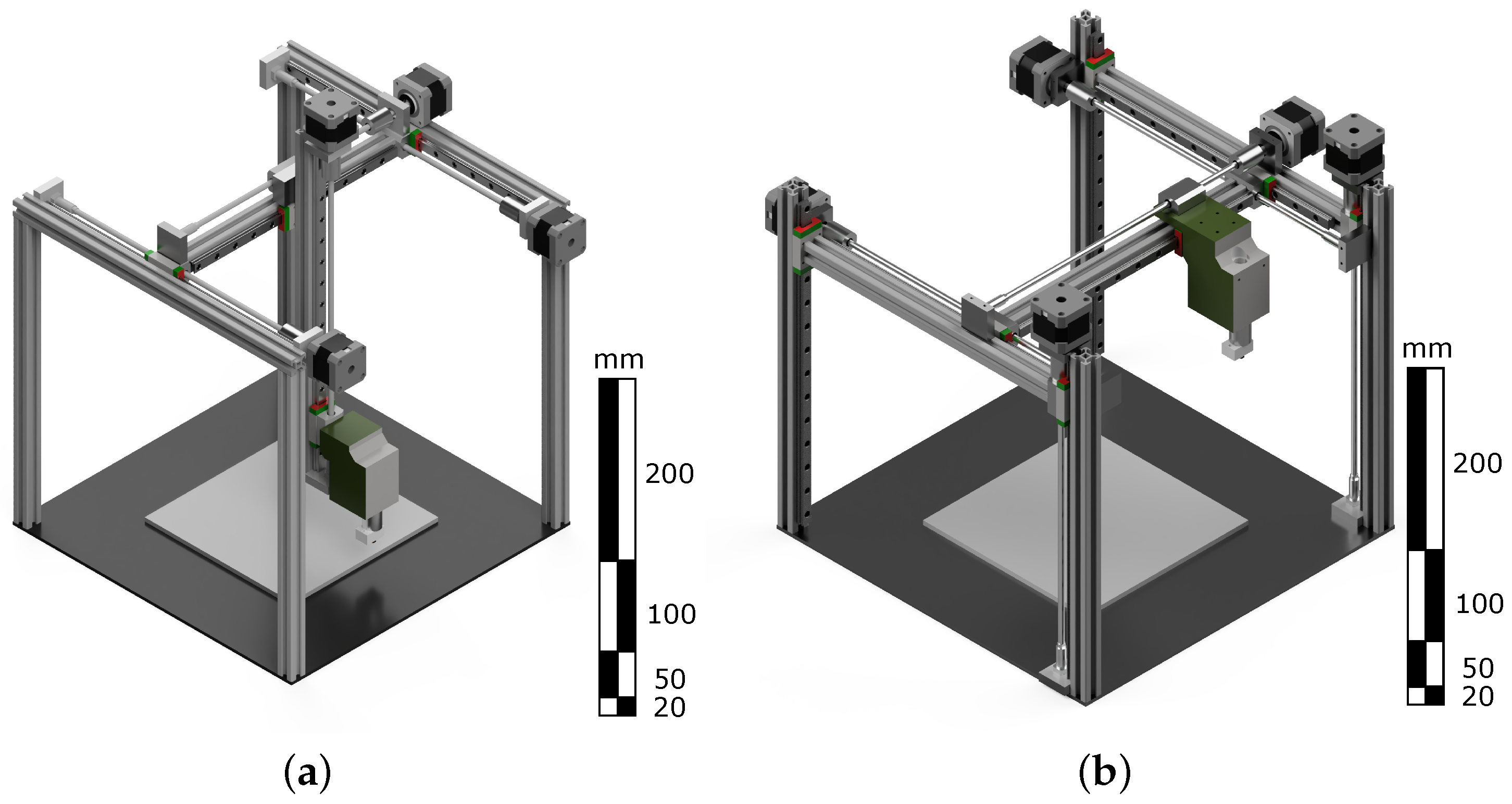
Table A2 of the kinematics are not used in practice, except for numbers three and four. Examples of a additive systems with closed X H , Y H and open Z H axes (see Figure A1a) are the machine painting systems [53,58]. The use of an open Z H here is due to the small movement requirement on the Z coordinate. Examples of 3D printers with closed axes X H , Y H , and open Z H (see Figure A1a) primarily are building 3D printers, e.g., from companies Specavia ATM [59], Winsun [60], COBOD [61], etc. Examples of 3D printers with closed axes X H , Y H , and Z H are VORON 2.4 [62] and a custom printer with Core-XYZ kinamtics [63].
Creating 3D printers with bed fixation is sometimes not a convenient technical solution but rather a forced one. The choice of this configuration for architectural printers can be explained by the fact that we can not move the platform on which the building stands.
Figure A1. 3D model of 3D printers with fixed axes X B , Y B , Z B and actuated axes X H , Y H , Z H (a) with closed X H , Y H and open Z H axes (b) with closed axes X H , Y H , Z H .
Applsci 12 04514 g0a1
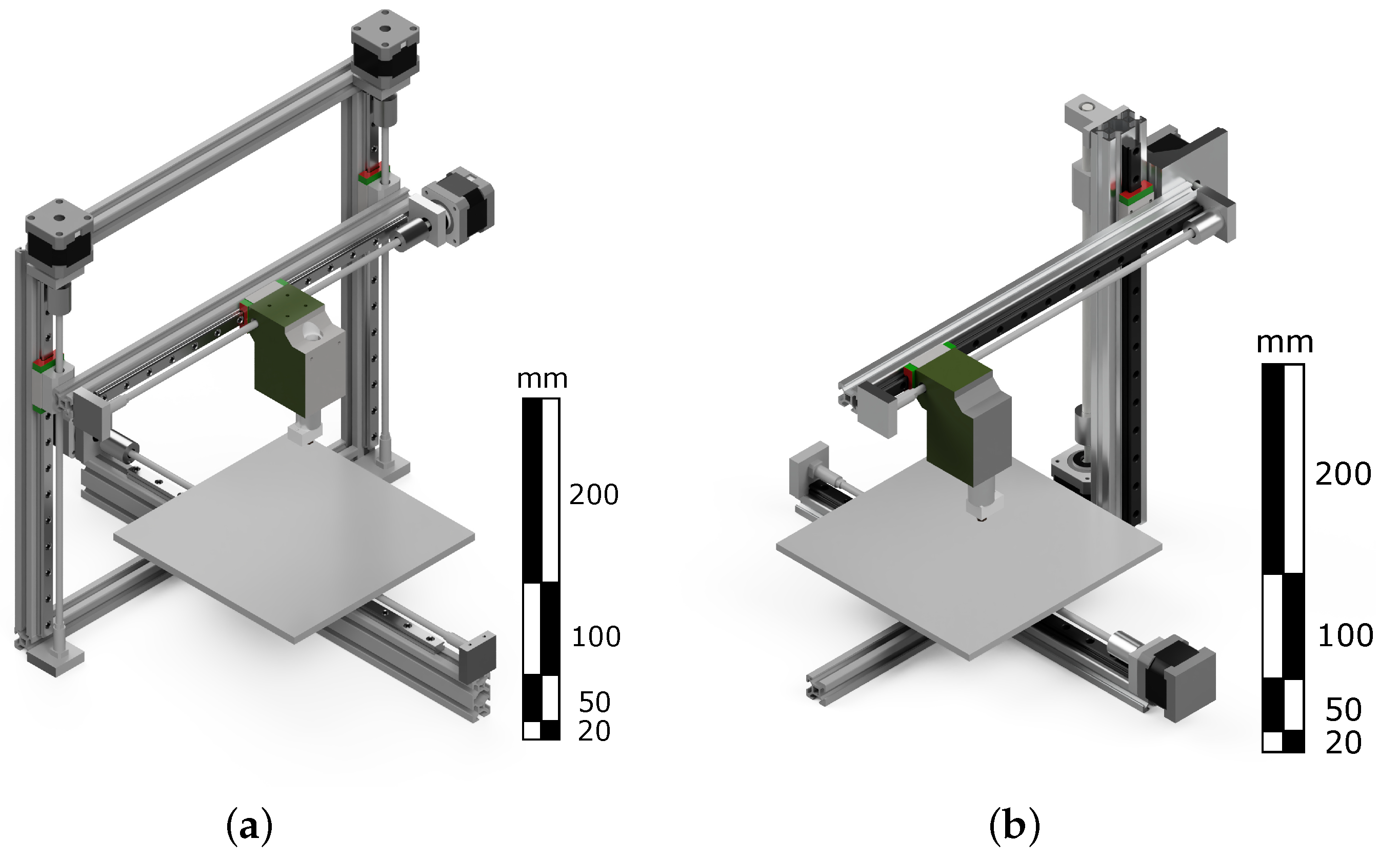
Table A3 illustrates two variants used in practice. Both variants are the most popular among all designs. An example of a 3D printer with closed X H , Y H and open Z B axes (see Figure A2a) is Anycubic 4max Pro [51] or Ultimaker 3. An example of a 3D printer with closed X H , Y H , Z B axes (see Figure A2b) is the Total Z Anyform 3D printer [64].These 3D printers differ only in the closed Z axis of the table, which affects the stiffness of the table. As a rule, 3D printers with a closed Z B axis are often significantly more expensive, which is due to using more precise ball screw drives instead of a trapezoidal screw and is not fully determined by the printer kinematics.
Figure A2. 3D model of 3D printers with fixed axes X B , Y B , Z H and actuated axes X H , Y H , Z B (a) with closed X H , Y H and open Z B axes (b) with closed X H , Y H , Z B axes.
Applsci 12 04514 g0a2
Table A4 shows two variants used in practice. The first variant is the one with closed axes X H , Y B and open Z H . This variant is trendy in the 3D-printers market due to its cheapness and simplicity of construction. Examples of a this type of 3D printers are Wanhao Duplicator i3 [65] and Anycubic i3 Mega [51] (see Figure A3a). The second variant with open X H , Z H axes and open Y B (see Figure A3b) is a simplified version of the previous model, and one of the cheapest variations of Cartesian 3D printers. An example of such a 3D printer is the Wanhao Duplicator i3 Mini 3D printer [66].
Figure A3. 3D model of 3D printers with fixed axes X B , Y H , Z B and actuated axes X H , Y B , Z H (a) with closed axes X H , Y B and open Z H (b) with open X H , Z H axes and open Y B .
Applsci 12 04514 g0a3
Examining the designs from Table A5, we found only one variant of the existing 3D printer with two actuated printbed axes. It is Felix 3.0 [67], a 3D printer with open Y B , Z B and closed X H (see Figure A4). The manufacturer claims that the 3D printer can develop a fairly high printing speed thanks to this design compared to its counterparts.
Figure A4. 3D model of 3D printer with fixed axes X B , Y H , Z H and actuated axes X H , Y B , Z B with closed axis X H , and open Y B , Z B .
Applsci 12 04514 g0a4
Three-dimensional printers with the designs shown in Table A6 and Table A7 were not found. Probably, such designs are not quite suitable for 3D printing. Moving the printing surface along all three axes can affect print quality since the printbed with the printed detail is much heavier than the printhead. However, it is possible that designs of this type are or will be used for other additive technologies, where complete fixation of the printhead is required due to its size and mass. A recent study published the design of a prototype 3D printer with a fully fixed extruder. However, this printer is not Cartesian and is not commercially available [68].
Now, make a complete classification scheme of the existing Cartesian 3D printers. It is given in Table A8. The classification scheme shows each case’s fixed and actuated axes and the closed and open axes for each actuated axis.
Table A8. Full classification of existing Cartesian 3D printers.
X B Y B Z B X H Y H Z H
1FF A O A C A O F
2F A C F A C F A O
3F A C F A O F A O
4FFF A C A C A O
5FFF A C A C A C
6FF A C A C A C F
7F A O A O A C FF
Only seven of the 40 possible kinematics designs (8 interchangeable) were identified among existing designs. Table A8 shows that the actuated axes are often closed for greater structural stiffness. Most of the actuated axes relate to the printhead.
Figure A5. Fixed axes X B , Y B , Z B and actuated axes X H , Y H , Z H . Existing designs are 3 and 4.
Applsci 12 04514 g0a5
Figure A6. Fixed axes X B , Y B , Z H and actuated axes X H , Y H , Z B . Existing designs are 3 and 4.
Applsci 12 04514 g0a6
Figure A7. Fixed axes X B , Y H , Z B and actuated axes X H , Y B , Z H . Existing designs are 1 and 3.
Applsci 12 04514 g0a7
Figure A8. Fixed axes X B , Y H , Z H and actuated axes X H , Y B , Z B . Existing design is 7.
Applsci 12 04514 g0a8
Figure A9. Fixed axes X H , Y H , Z B and actuated axes X B , Y B , Z H .
Applsci 12 04514 g0a9
Figure A10. Fixed axes X H , Y H , Z H and actuated axes X B , Y B , Z B .
Applsci 12 04514 g0a10
Figure A11. Classification scheme for existing Cartesian 3D printer designs, yellow C stands for closed axis, red O stands for open axis.
Applsci 12 04514 g0a11

References

  1. Qattawi, A.; Alrawi, B.; Guzman, A. Experimental optimization of fused deposition modelling processing parameters: A design-for-manufacturing approach. Procedia Manuf. 2017, 10, 791–803. [Google Scholar]
  2. Sharma, K.; Kumar, K.; Singh, K.R.; Rawat, M. Optimization of FDM 3D printing process parameters using Taguchi technique. IOP Conf. Ser. Mater. Sci. Eng. 2021, 1168, 012022. [Google Scholar] [CrossRef]
  3. Chand, R.; Sharma, V.S.; Trehan, R.; Gupta, M.K. A physical investigation of dimensional and mechanical characteristics of 3D printed nut and bolt for industrial applications. Rapid Prototyp. J. 2022. [Google Scholar] [CrossRef]
  4. Khorasani, M.; Ghasemi, A.; Rolfe, B.; Gibson, I. Additive manufacturing a powerful tool for the aerospace industry. Rapid Prototyp. J. 2021, 28, 87–100. [Google Scholar] [CrossRef]
  5. Dobra, A. General classification of robots. Size criteria. In Proceedings of the 2014 23rd International Conference on Robotics in Alpe-Adria-Danube Region (RAAD), Smolenice, Slovakia, 3–5 September 2014; pp. 1–6. [Google Scholar]
  6. Wilson, M. Implementation of Robot Systems: An Introduction to Robotics, Automation, and Successful Systems Integration in Manufacturing; Butterworth-Heinemann: Oxford, UK, 2014. [Google Scholar]
  7. Zhang, G.Q.; Li, X.; Boca, R.; Newkirk, J.; Zhang, B.; Fuhlbrigge, T.A.; Feng, H.K.; Hunt, N.J. Use of industrial robots in additive manufacturing-a survey and feasibility study. In Proceedings of the ISR/Robotik 2014—41st International Symposium on Robotics, Munich, Germany, 2–3 June 2014; pp. 1–6. [Google Scholar]
  8. Types Of FDM 3D Printers: Cartesian, Corexy, and More. Available online: https://all3dp.com/2/cartesian-3d-printer-delta-scara-belt-corexy-polar/ (accessed on 3 September 2021).
  9. Hsieh, C.T. Investigation of delta robot 3d printer for a good quality of printing. In Applied Mechanics and Materials; Trans Tech Publications Ltd.: Stafa-Zuerich, Switzerland, 2017; Volume 870, pp. 164–169. [Google Scholar]
  10. Carabin, G.; Scalera, L.; Wongratanaphisan, T.; Vidoni, R. An energy-efficient approach for 3D printing with a Linear Delta Robot equipped with optimal springs. Robot.-Comput.-Integr. Manuf. 2021, 67, 102045. [Google Scholar] [CrossRef]
  11. Vojić, S. Applications of collaborative industrial robots. Mach. Technol. Mater. 2020, 14, 96–99. [Google Scholar]
  12. Mohammad, A.E.K.; Hong, J.; Wang, D. Design of a force-controlled end-effector with low-inertia effect for robotic polishing using macro-mini robot approach. Robot.-Comput.-Integr. Manuf. 2018, 49, 54–65. [Google Scholar] [CrossRef]
  13. McClinton, E.; Wylie, B.; Moore, C.A. Creating a High and Homogenous Resolution Workspace for SCARA Based 3D Printers. IOP Conf. Ser. Mater. Sci. Eng. 2019, 689, 012021. [Google Scholar] [CrossRef]
  14. Alamsyah, F.A. The Kinematics Analysis of Robotic Arm manipulators Cylindrical Robot RPP Type for FFF 3D Print using Scilab. IOP Conf. Ser. Mater. Sci. Eng. 2019, 494, 012100. [Google Scholar] [CrossRef]
  15. Obi, M.U.; Pradel, P.; Sinclair, M.; Bibb, R. A bibliometric analysis of research in design for additive manufacturing. Rapid Prototyp. J. 2022. [Google Scholar] [CrossRef]
  16. Go, J.; Schiffres, S.N.; Stevens, A.G.; Hart, A.J. Rate limits of additive manufacturing by fused filament fabrication and guidelines for high-throughput system design. Addit. Manuf. 2017, 16, 1–11. [Google Scholar] [CrossRef]
  17. Löffler, R.; Koch, M. Innovative extruder concept for fast and efficient additive manufacturing. IFAC-PapersOnLine 2019, 52, 242–247. [Google Scholar] [CrossRef]
  18. Go, J.; Hart, A.J. Fast desktop-scale extrusion additive manufacturing. Addit. Manuf. 2017, 18, 276–284. [Google Scholar] [CrossRef] [Green Version]
  19. Xu, J.; Liu, K.; Liu, Z.; Zhang, F.; Zhang, S.; Tan, J. Electrothermal response optimization of nozzle structure for multi-material rapid prototyping based on fuzzy adaptive control. Rapid Prototyp. J. 2022. [Google Scholar] [CrossRef]
  20. Pilch, Z.; Domin, J.; Szłapa, A. The impact of vibration of the 3D printer table on the quality of print. In Proceedings of the 2015 Selected Problems of Electrical Engineering and Electronics (WZEE), Kielce, Poland, 17–19 September 2015; pp. 1–6. [Google Scholar]
  21. Ribeiro, G.d.S.; Silveira, Z. Structural and Modal Analysis of a Desktop 3-D Printer Considering an Interchangeable Mini Screw Extrusion Head. Available online: https://www.researchgate.net/publication/289484273_Structural_and_modal_analysis_of_a_desktop_3-D_printer_considering_an_interchangeable_mini_screw_extrusion_head (accessed on 1 April 2022).
  22. Verma, G. Autodesk Fusion 360 Black Book; BPB Publications: New Delhi, India, 2018. [Google Scholar]
  23. Okwudire, C.E.; Huggi, S.; Supe, S.; Huang, C.; Zeng, B. Low-level control of 3D printers from the cloud: A step toward 3D printer control as a service. Inventions 2018, 3, 56. [Google Scholar] [CrossRef] [Green Version]
  24. Levinskas, L. Research of Dimensional Accuracy and Surface Quality Dependency on Printing Speed of FDM 3D Printed Parts. Master’s Thesis, Kauno Technologijos Universitetas, Kaunas, Lithuania, 2019. [Google Scholar]
  25. Cohen, Z. Speed Limits: The Architectural Design Possibilities of the 3D Printed Corner. In Proceedings of the 107th Annual ACSA Conference Proceedings, Pittsburgh, PA, USA, 28–30 March 2019; ACSA Press: Washington, DC, USA, 2019. [Google Scholar]
  26. Srivastava, A.; Gautam, C.; Bhan, N.; Dayal, R. Vibration Analysis of Cantilever shaped 3D printers. IOP Conf. Ser. Mater. Sci. Eng. 2019, 594, 012020. [Google Scholar] [CrossRef] [Green Version]
  27. Cole-Pinnix, J. Optimal Control of Process Parameters in Additive Manufacturing (3D Printing) Using Six Sigma (DMAIC) Methodology. Ph.D. Thesis, North Carolina Agricultural and Technical State University, Greensboro, NC, USA, 2021. [Google Scholar]
  28. Galati, M.; Minetola, P.; Marchiandi, G.; Atzeni, E.; Calignano, F.; Salmi, A.; Iuliano, L. A methodology for evaluating the aesthetic quality of 3D printed parts. Procedia CIRP 2019, 79, 95–100. [Google Scholar] [CrossRef]
  29. Zhang, D.; Li, Z.; Qin, S.; Han, S. Optimization of vibration characteristics of fused deposition modeling color 3D printer based on modal and power spectrum method. Appl. Sci. 2019, 9, 4154. [Google Scholar] [CrossRef] [Green Version]
  30. Ford, D.G.; Myers, A.; Haase, F.; Lockwood, S.; Longstaff, A. Active vibration control for a CNC milling machine. Proc. Inst. Mech. Eng. Part C J. Mech. Eng. Sci. 2014, 228, 230–245. [Google Scholar] [CrossRef] [Green Version]
  31. Caixu, Y.; Haining, G.; Xianli, L.; Liang, S.Y.; Lihui, W. A review of chatter vibration research in milling. Chin. J. Aeronaut. 2019, 32, 215–242. [Google Scholar]
  32. Duan, M.; Yoon, D.; Okwudire, C.E. A limited-preview filtered B-spline approach to tracking control–With application to vibration-induced error compensation of a 3D printer. Mechatronics 2018, 56, 287–296. [Google Scholar] [CrossRef]
  33. Ramani, K.S.; Edoimioya, N.; Okwudire, C.E. A Robust Filtered Basis Functions Approach for Feedforward Tracking Control—With Application to a Vibration-Prone 3-D Printer. IEEE/ASME Trans. Mechatron. 2020, 25, 2556–2564. [Google Scholar] [CrossRef]
  34. Klipper Documentation. Resonance Compensation. Available online: https://www.klipper3d.org/Resonance_Compensation.html (accessed on 8 October 2021).
  35. Labuschagne, A.; van Rensburg, N.J.; Van der Merwe, A. Comparison of linear beam theories. Math. Comput. Model. 2009, 49, 20–30. [Google Scholar] [CrossRef]
  36. Fukuoka, T.; Nomura, M.; Sugano, N. Experimental investigation and finite element analysis of the free vibration problem of bolted joint by taking account of interface stiffness. J. Environ. Eng. 2009, 4, 101–111. [Google Scholar] [CrossRef] [Green Version]
  37. Worden, K.; Green, P. A machine learning approach to nonlinear modal analysis. Mech. Syst. Signal Process. 2017, 84, 34–53. [Google Scholar] [CrossRef]
  38. Hattori, G.; Serpa, A.L. Contact stiffness estimation in ANSYS using simplified models and artificial neural networks. Finite Elem. Anal. Des. 2015, 97, 43–53. [Google Scholar] [CrossRef] [Green Version]
  39. Zare, I.; Allen, M.S. Adapting a contact-mechanics algorithm to predict damping in bolted joints using quasi-static modal analysis. Int. J. Mech. Sci. 2021, 189, 105982. [Google Scholar] [CrossRef]
  40. Uwajambo, P.; Thakur, N. Numerical and Experimental Modal Analysis of CNC Machine; Blekinge Institute of Technology: Karlskrona, Sweden, 2021. [Google Scholar]
  41. Zhang, K.; Li, G.; Gong, J.; Wan, F. Modal Analysis of Bolted Structure Based on Equivalent Material of Joint Interface. Materials 2019, 12, 3004. [Google Scholar] [CrossRef] [Green Version]
  42. Jamia, N.; Jalali, H.; Taghipour, J.; Friswell, M.; Khodaparast, H.H. An equivalent model of a nonlinear bolted flange joint. Mech. Syst. Signal Process. 2021, 153, 107507. [Google Scholar] [CrossRef]
  43. Odrobiňák, J.; Idunk, R.; Bačinskỳ, T. Study on stiffness of composite beam-to-column joints. Procedia Eng. 2014, 91, 268–273. [Google Scholar] [CrossRef] [Green Version]
  44. Kopets, E.E.; Kolev, G.Y.; Vatnik, V.M.; Karimov, A.I.; Rybin, V.G. Mechanical Vibration Analysis of a Gantry 3D Printer. In Proceedings of the 2021 IEEE Conference of Russian Young Researchers in Electrical and Electronic Engineering (ElConRus), St. Petersburg, Russia, 26–29 January 2021; pp. 956–960. [Google Scholar]
  45. Han, S.M.; Benaroya, H.; Wei, T. Dynamics of transversely vibrating beams using four engineering theories. J. Sound Vib. 1999, 225, 935–988. [Google Scholar] [CrossRef] [Green Version]
  46. Karimov, A.I.; Kopets, E.; Nepomuceno, E.G.; Butusov, D. Integrate-and-Differentiate Approach to Nonlinear System Identification. Mathematics 2021, 9, 2999. [Google Scholar] [CrossRef]
  47. Marghitu, D.B. Kinematic Chains and Machine Components Design; Gulf Professional Publishing: Oxford, UK, 2005. [Google Scholar]
  48. Basova, Y.; Nutsubidze, K.; Ivanova, M.; Slipchenko, S.; Kotliar, A. Design and numerical simulation of the new design of the gripper for manipulating of the rotational parts. Diagnostyka 2018, 19, 11–18. [Google Scholar] [CrossRef]
  49. Zhang, H.; Zhao, W.; Du, C.; Liu, H.; Zhang, J. Dynamic modeling and analysis for gantry-type machine tools considering the effect of axis coupling force on the slider–guide joints’ stiffness. Proc. Inst. Mech. Eng. Part B J. Eng. Manuf. 2016, 230, 2036–2046. [Google Scholar] [CrossRef]
  50. Original Prusa i3 MK3S+ Kit. Available online: https://www.prusa3d.com/product/original-prusa-i3-mk3s-kit-3/ (accessed on 24 April 2022).
  51. Anycubic 4Max Pro 2.0. Available online: https://www.anycubic.com/collections/max-series (accessed on 3 September 2021).
  52. Sovol SV03. Available online: https://sovol3d.com/products/sv03 (accessed on 24 April 2022).
  53. Karimov, A.I.; Kopets, E.E.; Rybin, V.G.; Leonov, S.V.; Voroshilova, A.I.; Butusov, D.N. Advanced tone rendition technique for a painting robot. Robot. Auton. Syst. 2019, 115, 17–27. [Google Scholar] [CrossRef]
  54. Batley, S. Classification in Theory and Practice; Chandos Publishing: Oxford, UK, 2014. [Google Scholar]
  55. Wang, X.; Baron, L.; Cloutier, G. Topology of serial and parallel manipulators and topological diagrams. Mech. Mach. Theory 2008, 43, 754–770. [Google Scholar] [CrossRef]
  56. Müller, A. Generic mobility of rigid body mechanisms. Mech. Mach. Theory 2009, 44, 1240–1255. [Google Scholar] [CrossRef]
  57. Lu, Y.; Hu, B.; Sun, T. Analyses of velocity, acceleration, statics, and workspace of a 2 (3-SPR) serial-parallel manipulator. Robotica 2009, 27, 529–538. [Google Scholar] [CrossRef]
  58. Helms, C. Van gobot. Sci. Am. 2018, 318, 9. [Google Scholar]
  59. Specavia ATM. Available online: http://specavia.pro/catalog/ (accessed on 3 September 2021).
  60. Winsun 3D Printer. Available online: http://www.winsun3d.com/En/ (accessed on 3 September 2021).
  61. The BOD. Europe’s First 3D Printed Building. Available online: https://cobod.com/the-bod/ (accessed on 3 September 2021).
  62. Voron 2.4 3D Printer Assembly Manual. Available online: https://github.com/VoronDesign/Voron-2/raw/Voron2.4/Docs/2.4_Assembly_Manual.pdf (accessed on 3 September 2021).
  63. Core-XYZ First Motion with Modded REPETIER Firmware!—Video Uploaded by 1kreature. Available online: https://youtu.be/Ii0lUfQ8pJI (accessed on 3 September 2021).
  64. 3D-printer AnyForm L250-G3(2X). Available online: https://totalz.ru/products/equipment/universal-fdm/anyform-l250-g3-2x/ (accessed on 3 September 2021).
  65. Wanhao 3D Printer. Available online: https://https://www.wanhao3dprinter.com/Index.html/ (accessed on 3 September 2021).
  66. Wanhao i3 Mini. Available online: https://wanhao.store/products/wanaho-i3-mini/ (accessed on 3 September 2021).
  67. Felix Pro 3 Highlights. Available online: https://www.felixprinters.com/pro-3-highlights/ (accessed on 3 September 2021).
  68. Tlegenov, Y.; Hong, G.S.; Lu, W.F. Nozzle condition monitoring in 3D printing. Robot.-Comput.-Integr. Manuf. 2018, 54, 45–55. [Google Scholar] [CrossRef]
Figure 1. Example of corner swell (upper box) and ghosting (lower box). Arrows mark typical variants of these defects.
Applsci 12 04514 g001
Figure 2. Experimental frequencies of the beam. (Top): one hidden bracket for fastening to a base is used, several peaks emerge because of the joint stiffness non-linearity [46]. (Bottom): two hidden brackets are used, the vibration is close to harmonic.
Applsci 12 04514 g002
Figure 3. Examples of kinematic schemes for Cartesian 3D printers. Rectangles denote prismatic joints, circles denote spherical joints, a black triangle denotes the printhead, and a black parallelepiped denotes the printbed. Panels (ac) refer to functional kinematic schemes, while the panels (df) additionally show frame and guide joints that cannot be considered absolutely stiff.
Applsci 12 04514 g003
Figure 4. Practical implementation of a Cartesian system. Panel (a) shows a functional kinematic scheme of a Cartesian gantry CNC machine and panel (b) gives a detailed kinematic scheme of its implementation with actuated prismatic joints (shown with white rectangles) and passive rail guides (shown with grey rectangles). Circles denote passive spherical joints with internal stiffeners, a black triangle denotes the printhead, and a black parallelepiped denotes the printbed.
Applsci 12 04514 g004
Figure 5. Model of the beam.
Applsci 12 04514 g005
Figure 6. Model of the portal.
Applsci 12 04514 g006
Figure 7. Model of the parallelepiped.
Applsci 12 04514 g007
Figure 8. Anycubic i3 Mega kinematic scheme.
Applsci 12 04514 g008
Figure 9. (a) Model of the 3D printer Anycubic i3 Mega. A circle marks a place of the accelerometer mounting, an arrow marks the direction of axis sensitivity (b) Example of the accelerometer mounting.
Applsci 12 04514 g009
Figure 10. The first mode of the Anycubic i3 Mega 3D printer.
Applsci 12 04514 g010
Figure 11. Common printer designs used in the investigation.
Applsci 12 04514 g011
Figure 12. Lowest normal modes of 3D printer structures found by the FEM and by the proposed approach based on a flexible joint model.
Applsci 12 04514 g012
Table 1. The first mode of the Anycubic i3 Mega 3D printer.
Z, mmTheoretical, HzExperimental, HzRelative Error, %
013.8513.363.54
1013.6713.193.52
2013.4912.785.31
3013.3112.843.48
4013.1213.070.38
5012.9212.622.38
6012.7312.402.58
7012.5312.123.26
8012.3311.992.79
9012.1411.941.62
10011.9411.910.23
12011.7411.502.07
13011.5511.792.08
14011.3611.894.69
15011.1611.573.59
16010.9811.222.18
17010.7911.365.27
18010.6110.973.41
19010.4311.045.82
20010.2610.562.97
Table 2. Parameters of the evaluated design.
ParameterValueUnits
Profile angle stiffness k P 3700N·m/rad
Linear guide mount angle stiffness k L 2000N·m/rad
Profile density ρ P 0.85kg/m
Linear rail guide density ρ R 1.45kg/m
Linear 8 mm guide density ρ G 0.4kg/m
Stepper motor mass M M 0.26kg
Printhead mass M H 0.7kg
Printbed mass M B 0.4kg
Vertical beam length L 1 0.4m
Z position of the printbed L 2 0.3m
Horizontal beam length L h 0.4m
Table 3. Modes 1–3 of the printers obtained by the FEM and the lowest mode by the proposed method.
Mode 1, HzMode 2, HzMode 3, HzProposed Method, Hz
131.1231.3853.9931.59
242.9745.5095.3724.14
358.0467.02103.517.81
460.6284.89117.424.83
532.8340.8177.7125.67
631.4536.1260.5836.72
748.7350.3896.9727.93
Table 4. The cost of a 3D printer in Figure A3a.
ComponentAmountCost of 1 Piece, $Total Cost, $Cost Ratio
Aluminum profile2400 mm3–5 (1000 mm)7.2–126–3%
Lead screw5 pc.2–510–258–6%
Rail guide system4 pc.7–2528–10022%
Stepper motor4 pc.5–1520–6015–13%
PSU1 pc.5–205–204%
Print bed1 pc.15–5015–5012–11%
Print Head1 pc.15–8015–8012–18%
Controller Board1 pc.30–10030–10023–22%
All components excluding additional spare parts130.2–447
Publisher’s Note: MDPI stays neutral with regard to jurisdictional claims in published maps and institutional affiliations.

