
Ultrasound Localization Microscopy in Liquid Metal Flows

 , , , , , and
Abstract
:1. Introduction
1.1. Motivation
1.2. State of the Art
1.3. Aim and Outline
2. Ultrasound Localization Microscopy
2.1. Ultrafast Imaging
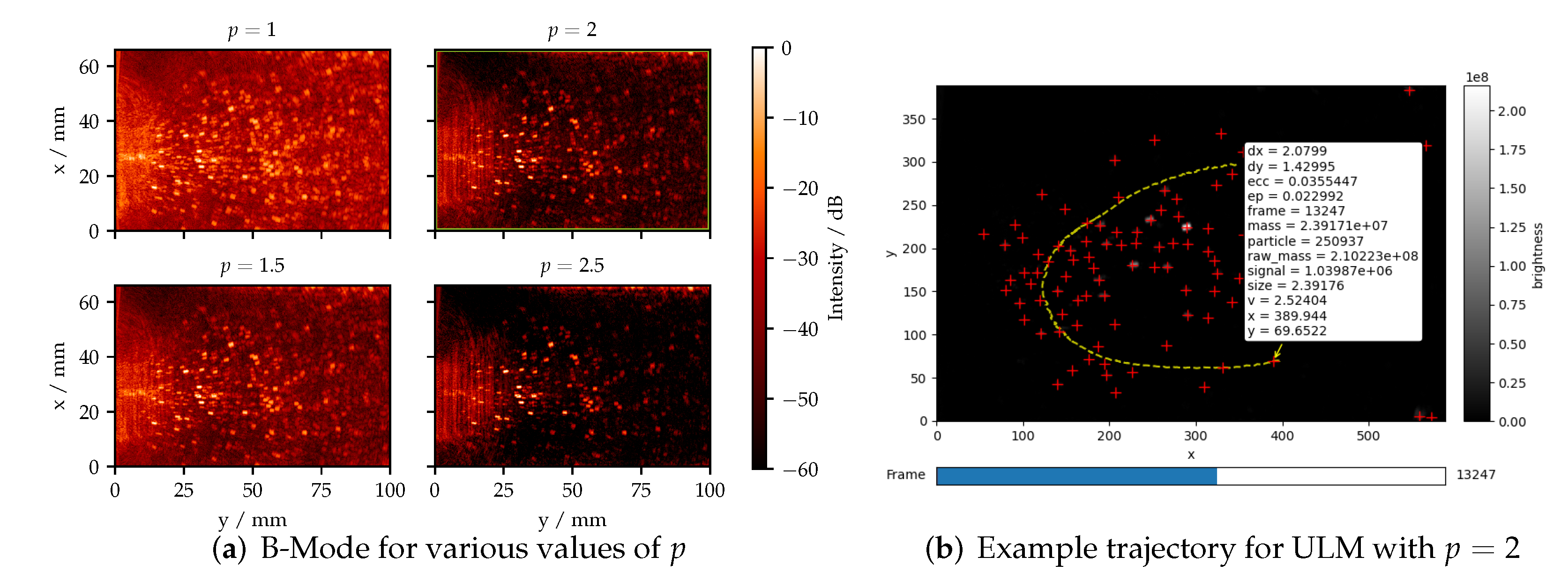
2.2. Nonlinear Beamforming
2.3. Particle Localization and Tracking
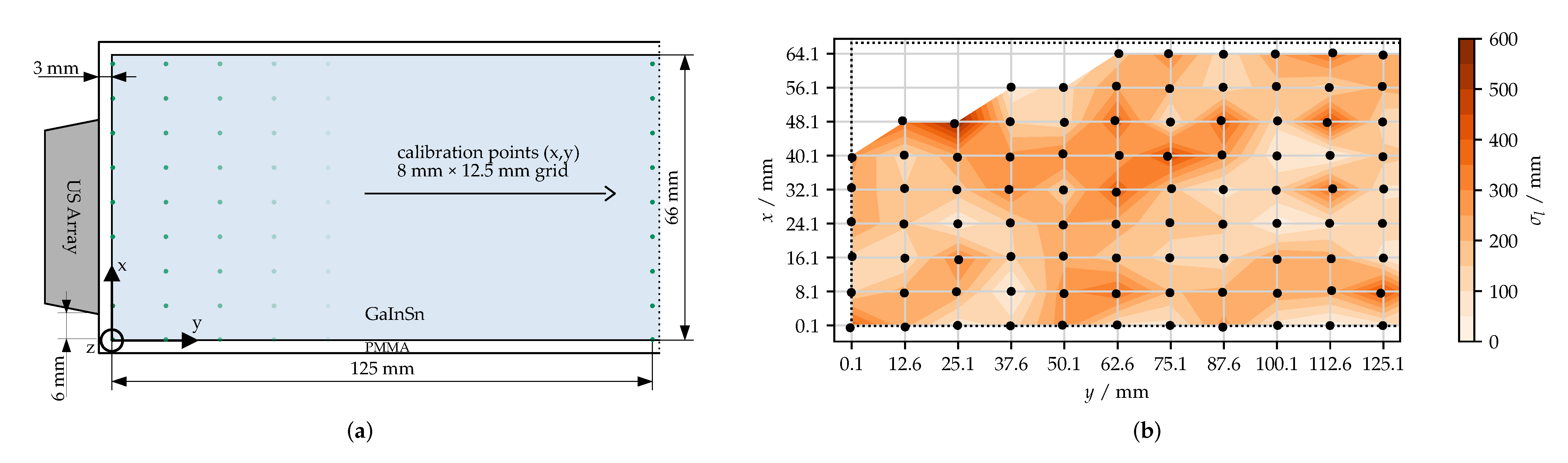
3. Characterization of the Spatial Resolution
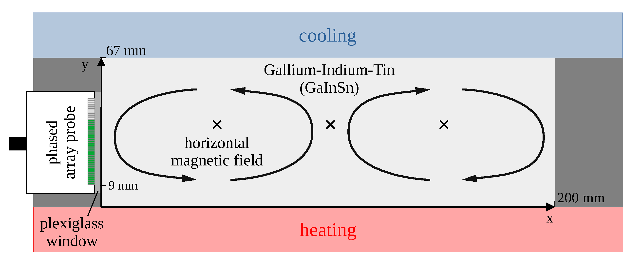
4. Test Case: Rayleigh–Bénard Convection Experiment
4.1. Set-Up
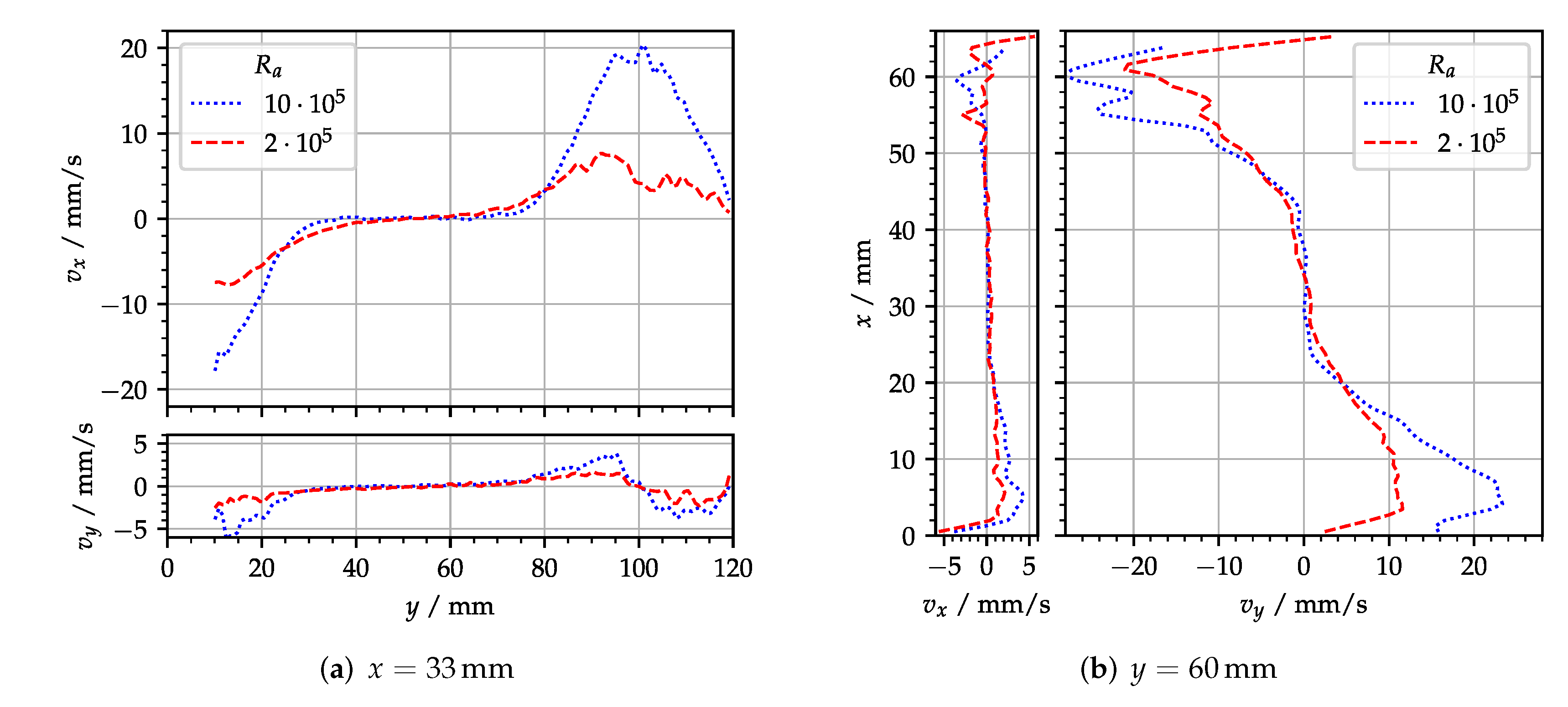
4.2. Application
5. Conclusions
Supplementary Materials
Author Contributions
Funding
Institutional Review Board Statement
Informed Consent Statement
Data Availability Statement
Acknowledgments
Conflicts of Interest
References
- King, E.M.; Soderlund, K.M.; Christensen, U.R.; Wicht, J.; Aurnou, J.M. Convective heat transfer in planetary dynamo models. Geochem. Geophys. Geosyst. 2010, 11. [Google Scholar] [CrossRef]
- Schubert, G.; Soderlund, K.M. Planetary magnetic fields: Observations and models. Phys. Earth Planet. Inter. 2011, 187, 92–108. [Google Scholar] [CrossRef]
- DeLovato, N.; Sundarnath, K.; Cvijovic, L.; Kota, K.; Kuravi, S. A review of heat recovery applications for solar and geothermal power plants. Renew. Sustain. Energy Rev. 2019, 114, 109329. [Google Scholar] [CrossRef]
- Flesch, J.; Marocco, L.; Fritsch, A.; Niedermeier, K.; Wetzel, T. Entropy Generation Minimization Analysis of Solar Salt, Sodium, and Lead–Bismuth Eutectic as High Temperature Heat Transfer Fluids. J. Heat Transf. 2020, 142, 042103. [Google Scholar] [CrossRef]
- Ahlers, G.; Grossmann, S.; Lohse, D. Heat transfer and large scale dynamics in turbulent Rayleigh-Bénard convection. Rev. Mod. Phys. 2009, 81, 503–537. [Google Scholar] [CrossRef] [Green Version]
- Chillà, F.; Schumacher, J. New perspectives in turbulent Rayleigh-Bénard convection. Eur. Phys. J. E 2012, 35, 1–25. [Google Scholar] [CrossRef] [Green Version]
- Aurnou, J.M.; Horn, S.; Julien, K. Connections between nonrotating, slowly rotating, and rapidly rotating turbulent convection transport scalings. Phys. Rev. Res. 2020, 2, 043115. [Google Scholar] [CrossRef]
- Vogt, T.; Ishimi, W.; Yanagisawa, T.; Tasaka, Y.; Sakuraba, A.; Eckert, S. Transition between quasi-two-dimensional and three-dimensional Rayleigh-Bénard convection in a horizontal magnetic field. Phys. Rev. Fluids 2018, 3, 013503. [Google Scholar] [CrossRef]
- Yang, J.; Vogt, T.; Eckert, S. Transition from steady to oscillating convection rolls in Rayleigh-Bénard convection under the influence of a horizontal magnetic field. Phys. Rev. Fluids 2021, 6, 023502. [Google Scholar] [CrossRef]
- Akashi, M.; Yanagisawa, T.; Sakuraba, A.; Schindler, F.; Horn, S.; Vogt, T.; Eckert, S. Jump rope vortex flow in liquid metal Rayleigh–Bénard convection in a cuboid container of aspect ratio. J. Fluid Mech. 2022, 932, A27. [Google Scholar] [CrossRef]
- Horn, S.; Schmid, P.J.; Aurnou, J.M. Unravelling the large-scale circulation modes in turbulent Rayleigh-Bénard convection. Europhys. Lett. 2022, 136, 14003. [Google Scholar] [CrossRef]
- Vogt, T.; Horn, S.; Grannan, A.M.; Aurnou, J.M. Jump rope vortex in liquid metal convection. Proc. Natl. Acad. Sci. USA 2018, 115, 12674–12679. [Google Scholar] [CrossRef] [PubMed] [Green Version]
- Zürner, T.; Schindler, F.; Vogt, T.; Eckert, S.; Schumacher, J. Combined measurement of velocity and temperature in liquid metal convection. J. Fluid Mech. 2019, 876, 1108–1128. [Google Scholar] [CrossRef] [Green Version]
- Vogt, T.; Yang, J.C.; Schindler, F.; Eckert, S. Free-fall velocities and heat transport enhancement in liquid metal magneto-convection. J. Fluid Mech. 2021, 915, A68. [Google Scholar] [CrossRef]
- Takeda, Y.; Kikura, H. Flow mapping of the mercury flow. Exp. Fluids 2002, 32, 161–169. [Google Scholar] [CrossRef]
- Wang, B.; Kelley, D.H. Microscale mechanisms of ultrasound velocity measurement in metal melts. Flow Meas. Instrum. 2021, 81, 102010. [Google Scholar] [CrossRef]
- Takeda, Y. Development of an ultrasound velocity profile monitor. Nucl. Eng. Des. 1991, 126, 277–284. [Google Scholar] [CrossRef]
- Franke, S.; Büttner, L.; Czarske, J.; Räbiger, D.; Eckert, S. Ultrasound Doppler system for two-dimensional flow mapping in liquid metals. Flow Meas. Instrum. 2010, 21, 402–409. [Google Scholar] [CrossRef]
- Büttner, L.; Nauber, R.; Burger, M.; Räbiger, D.; Franke, S.; Eckert, S.; Czarske, J. Dual-plane ultrasound flow measurements in liquid metals. Meas. Sci. Technol. 2013, 24, 055302. [Google Scholar] [CrossRef]
- Nauber, R.; Büttner, L.; Czarske, J. Measurement uncertainty analysis of field-programmable gate-array-based, real-time signal processing for ultrasound flow imaging. J. Sens. Sens. Syst. 2020, 9, 227–238. [Google Scholar] [CrossRef]
- Tanter, M.; Bercoff, J.; Sandrin, L.; Fink, M. Ultrafast compound imaging for 2-D motion vector estimation: Application to transient elastography. IEEE Trans. Ultrason. Ferroelectr. Freq. Control 2002, 49, 1363–1374. [Google Scholar] [CrossRef] [PubMed]
- Udesen, J.; Gran, F.; Hansen, K.L.; Jensen, J.A.; Thomsen, C.; Nielsen, M.B. High frame-rate blood vector velocity imaging using plane waves: Simulations and preliminary experiments. IEEE Trans. Ultrason. Ferroelectr. Freq. Control 2008, 55, 1729–1743. [Google Scholar] [CrossRef] [PubMed]
- Montaldo, G.; Tanter, M.; Bercoff, J.; Benech, N.; Fink, M. Coherent plane-wave compounding for very high frame rate ultrasonography and transient elastography. IEEE Trans. Ultrason. Ferroelectr. Freq. Control 2009, 56, 489–506. [Google Scholar] [CrossRef] [PubMed]
- Poelma, C.; van der Mijle, R.; Mari, J.; Tang, M.X.; Weinberg, P.; Westerweel, J. Ultrasound imaging velocimetry: Toward reliable wall shear stress measurements. Eur. J. Mech.- B/Fluids 2012, 35, 70–75. [Google Scholar] [CrossRef]
- Leow, C.H.; Bazigou, E.; Eckersley, R.J.; Yu, A.C.; Weinberg, P.D.; Tang, M.X. Flow Velocity Mapping Using Contrast Enhanced High-Frame-Rate Plane Wave Ultrasound and Image Tracking: Methods and Initial in Vitro and in Vivo Evaluation. Ultrasound Med. Biol. 2015, 41, 2913–2925. [Google Scholar] [CrossRef] [Green Version]
- Poelma, C. Ultrasound imaging velocimetry: A review. Exp. Fluids 2017, 58, 3. [Google Scholar] [CrossRef] [Green Version]
- Weik, D.; Nauber, R.; Kupsch, C.; Büttner, L.; Czarske, J. Uncertainty Quantification of Ultrasound Image Velocimetry for Liquid Metal Flow Mapping. IEEE Trans. Instrum. Meas. 2021, 70, 1–11. [Google Scholar] [CrossRef]
- Siepmann, M.; Schmitz, G.; Bzyl, J.; Palmowski, M.; Kiessling, F. Imaging tumor vascularity by tracing single microbubbles. In Proceedings of the 2011 IEEE International Ultrasonics Symposium, Orlando, FL, USA, 18–21 October 2011; pp. 1906–1909. [Google Scholar]
- Desailly, Y.; Couture, O.; Fink, M.; Tanter, M. Sono-activated ultrasound localization microscopy. Appl. Phys. Lett. 2013, 103, 174107. [Google Scholar] [CrossRef]
- Ackermann, D.; Schmitz, G. Detection and Tracking of Multiple Microbubbles in Ultrasound B-Mode Images. IEEE Trans. Ultrason. Ferroelectr. Freq. Control 2016, 63, 72–82. [Google Scholar] [CrossRef]
- Diamantis, K.; Greenaway, A.H.; Anderson, T.; Jensen, J.A.; Dalgarno, P.A.; Sboros, V. Super-Resolution Axial Localization of Ultrasound Scatter Using Multi-Focal Imaging. IEEE Trans. Biomed. Eng. 2018, 65, 1840–1851. [Google Scholar] [CrossRef] [Green Version]
- Betzig, E.; Patterson, G.H.; Sougrat, R.; Lindwasser, O.W.; Olenych, S.; Bonifacino, J.S.; Davidson, M.W.; Lippincott-Schwartz, J.; Hess, H.F. Imaging intracellular fluorescent proteins at nanometer resolution. Science 2006, 313, 1642–1645. [Google Scholar] [CrossRef] [PubMed] [Green Version]
- Desailly, Y.; Pierre, J.; Couture, O.; Tanter, M. Resolution limits of ultrafast ultrasound localization microscopy. Phys. Med. Biol. 2015, 60, 8723. [Google Scholar] [CrossRef] [PubMed]
- Bouakaz, A.; Frigstad, S.; Ten Cate, F.J.; de Jong, N. Super harmonic imaging: A new imaging technique for improved contrast detection. Ultrasound Med. Biol. 2002, 28, 59–68. [Google Scholar] [CrossRef]
- Errico, C.; Pierre, J.; Pezet, S.; Desailly, Y.; Lenkei, Z.; Couture, O.; Tanter, M. Ultrafast ultrasound localization microscopy for deep super-resolution vascular imaging. Nature 2015, 527, 499–502. [Google Scholar] [CrossRef]
- Christensen-Jeffries, K.; Couture, O.; Dayton, P.A.; Eldar, Y.C.; Hynynen, K.; Kiessling, F.; O’Reilly, M.; Pinton, G.F.; Schmitz, G.; Tang, M.X.; et al. Super-resolution Ultrasound Imaging. Ultrasound Med. Biol. 2020, 46, 865–891. [Google Scholar] [CrossRef] [Green Version]
- Demené, C.; Robin, J.; Dizeux, A.; Heiles, B.; Pernot, M.; Tanter, M.; Perren, F. Transcranial ultrafast ultrasound localization microscopy of brain vasculature in patients. Nat. Biomed. Eng. 2021, 5, 219–228. [Google Scholar] [CrossRef]
- Kupsch, C.; Feierabend, L.; Nauber, R.; Büttner, L.; Czarske, J. Ultrasound Super-Resolution Flow Measurement of Suspensions in Narrow Channels. IEEE Trans. Ultrason. Ferroelectr. Freq. Control 2021, 68, 807–817. [Google Scholar] [CrossRef]
- Thieme, N.; Keil, M.; Meier, D.; Bönisch, P.; Dadzis, K.; Pätzold, O.; Stelter, M.; Büttner, L.; Czarske, J. Directional solidification of gallium under time-dependent magnetic fields with in situ measurements of the melt flow and the solid-liquid interface. J. Cryst. Growth 2019, 522, 221–229. [Google Scholar] [CrossRef]
- Mäder, K.; Nauber, R.; Galindo, V.; Beyer, H.; Büttner, L.; Eckert, S.; Czarske, J. Phased Array Ultrasound System for Planar Flow Mapping in Liquid Metals. IEEE Trans. Ultrason. Ferroelectr. Freq. Control 2017, 64, 1327–1335. [Google Scholar] [CrossRef]
- Mucci, R. A comparison of efficient beamforming algorithms. IEEE Trans. Acoust. Speech Signal Process. 1984, 32, 548–558. [Google Scholar] [CrossRef]
- Matrone, G.; Savoia, A.S.; Caliano, G.; Magenes, G. The Delay Multiply and Sum Beamforming Algorithm in Ultrasound B-Mode Medical Imaging. IEEE Trans. Med. Imaging 2015, 34, 940–949. [Google Scholar] [CrossRef] [PubMed]
- Mozaffarzadeh, M.; Mahloojifar, A.; Orooji, M.; Adabi, S.; Nasiriavanaki, M. Double-Stage Delay Multiply and Sum Beamforming Algorithm: Application to Linear-Array Photoacoustic Imaging. IEEE Trans. Biomed. Eng. 2018, 65, 31–42. [Google Scholar] [CrossRef] [PubMed] [Green Version]
- Polichetti, M.; Varray, F.; Béra, J.C.; Cachard, C.; Nicolas, B. A nonlinear beamformer based on p-th root compression—Application to plane wave ultrasound imaging. Appl. Sci. 2018, 8, 599. [Google Scholar] [CrossRef] [Green Version]
- Grüter, L.; Bilsing, C.; Radner, H.; Weik, D. PtvPy v0.10.2. Zenodo 2022. [Google Scholar] [CrossRef]
- Allan, D.B.; Caswell, T.; Keim, N.C.; van der Wel, C.M.; Verweij, R.W. Soft-Matter/Trackpy: Trackpy v0.5.0. Zenodo 2021. [Google Scholar] [CrossRef]
- Crocker, J.C.; Grier, D.G. Methods of digital video microscopy for colloidal studies. J. Colloid Interface Sci. 1996, 179, 298–310. [Google Scholar] [CrossRef] [Green Version]
- Couture, O.; Hingot, V.; Heiles, B.; Muleki-Seya, P.; Tanter, M. Ultrasound Localization Microscopy and Super-Resolution: A State of the Art. IEEE Trans. Ultrason. Ferroelectr. Freq. Control 2018, 65, 1304–1320. [Google Scholar] [CrossRef] [Green Version]
- Tasaka, Y.; Igaki, K.; Yanagisawa, T.; Vogt, T.; Zuerner, T.; Eckert, S. Regular flow reversals in Rayleigh-Bénard convection in a horizontal magnetic field. Phys. Rev. E 2016, 93, 043109. [Google Scholar] [CrossRef] [Green Version]
- Harput, S.; Christensen-Jeffries, K.; Ramalli, A.; Brown, J.; Zhu, J.; Zhang, G.; Leow, C.H.; Toulemonde, M.; Boni, E.; Tortoli, P.; et al. 3-D Super-Resolution Ultrasound Imaging with a 2-D Sparse Array. IEEE Trans. Ultrason. Ferroelectr. Freq. Control 2020, 67, 269–277. [Google Scholar] [CrossRef]
- Matrone, G.; Bell, M.A.L.; Ramalli, A. Spatial Coherence Beamforming With Multi-Line Transmission to Enhance the Contrast of Coherent Structures in Ultrasound Images Degraded by Acoustic Clutter. IEEE Trans. Ultrason. Ferroelectr. Freq. Control 2021, 68, 3570–3582. [Google Scholar] [CrossRef]
- Youn, J.; Ommen, M.L.; Stuart, M.B.; Thomsen, E.V.; Larsen, N.B.; Jensen, J.A. Detection and Localization of Ultrasound Scatterers Using Convolutional Neural Networks. IEEE Trans. Med. Imaging 2020, 39, 3855–3867. [Google Scholar] [CrossRef] [PubMed]
- Taghavi, I.; Andersen, S.B.; Hoyos, C.A.V.; Schou, M.; Gran, F.; Hansen, K.L.; Nielsen, M.B.; Sørensen, C.M.; Stuart, M.B.; Jensen, J.A. Ultrasound super-resolution imaging with a hierarchical Kalman tracker. Ultrasonics 2022, 122, 106695. [Google Scholar] [CrossRef] [PubMed]


Publisher’s Note: MDPI stays neutral with regard to jurisdictional claims in published maps and institutional affiliations. |
© 2022 by the authors. Licensee MDPI, Basel, Switzerland. This article is an open access article distributed under the terms and conditions of the Creative Commons Attribution (CC BY) license (https://creativecommons.org/licenses/by/4.0/).
Share and Cite
Weik, D.; Grüter, L.; Räbiger, D.; Singh, S.; Vogt, T.; Eckert, S.; Czarske, J.; Büttner, L. Ultrasound Localization Microscopy in Liquid Metal Flows. Appl. Sci. 2022, 12, 4517. https://doi.org/10.3390/app12094517
Weik D, Grüter L, Räbiger D, Singh S, Vogt T, Eckert S, Czarske J, Büttner L. Ultrasound Localization Microscopy in Liquid Metal Flows. Applied Sciences. 2022; 12(9):4517. https://doi.org/10.3390/app12094517
Chicago/Turabian StyleWeik, David, Lars Grüter, Dirk Räbiger, Sanjay Singh, Tobias Vogt, Sven Eckert, Jürgen Czarske, and Lars Büttner. 2022. "Ultrasound Localization Microscopy in Liquid Metal Flows" Applied Sciences 12, no. 9: 4517. https://doi.org/10.3390/app12094517