Optimized Pilot Point Emplacement Based Groundwater Flow Calibration Method for Heterogeneous Small-Scale Area

Abstract

Groundwater flow modeling in a small-scale area requires practical techniques to obtain high accuracy results. The effectiveness of the model calibration is the most challenging for simulating the hydraulic head. In pursuit of this, we proposed an optimized groundwater flow calibration method based on the pilot point emplacement technique for a 3D small-scale area in this work. Subsequently, two emplacement structures were tested during the experimentation, the regular pilot point placement, and the middle head measurement down gradient (MHMDG) placement with two different densities. The parameter estimation (PEST) numerical code applying the kriging interpolation was used to estimate the hydraulic conductivity field by MODFLOW. Moreover, geological SGrid models were chosen for the conceptual model. Thirty-seven observation wells were used for experimental simulations to test the proposed method in a heterogeneous confined aquifer. The result shows that the small-scale modeling was complicated, and the studying area presented a significant heterogeneity in horizontal hydraulic conductivity. The middle head measurement down gradient (MHMDG) pilot point case with the larger density gave the best R-squared 0.901 and minimum residual error of 0.0053 m compared to 0.880 and 0.078 m, respectively, for the regular placement. The calibration accuracy depended on the frequency and the emplacement of the pilot point. Therefore, the initial value should be technically selected to minimize the computation burden. The proposed techniques help to improve the groundwater flow model calibration based on the pilot point methodology for groundwater resources management.

1. Introduction

Groundwater flow modeling is the mathematical simulation of the actual condition of an aquifer considering all related hydrogeological parameters [1]. It remains one of the most effective decision-making tools for water resources management. It can be categorized from various techniques, such as calculating the hydraulic head, mapping the potential recharge zone for water supply management [2], calculating the water budget, or mapping the hydraulic change by estimating the hydraulic storage using GIS or mapping satellite data [3]. Theoretically, a satisfying model presents an exclusively less residual error. This accuracy concern could be approached through the calibration process [4].

In general, model calibration entails modifying model input data to make the model more accurately reflect observed heads and flows. The input parameters could be hydrological, or soil features essential to understanding the relationship between soil and groundwater [5]. Using nonlinear regression statistical techniques, parameters can be calibrated manually or automatically. The manual calibration helps to minimize the residual between the observed value of the hydraulic head and the numerically calculated value; however, the process is relatively laborious. Compared to manual calibration, the automatic calibration is fast and trustworthy despite unrealistic output probability. In the past, several automated calibration methods have been proposed, such as the global optimization method [6], the Bayesian-based calibration method that adopts a Gaussian process error model [7], and the pilot point calibration method.

Doherty, J. [8] introduced an automatic calibration technique using pilot points to estimate the hydraulic conductivity field on a heterogeneous model. In nonlinear geostatistical calibration, the pilot point approach is often utilized to fit the aquifer response better. Regularization, in addition to the calibration methodology, was also conducted a few years later to obtain the uniqueness of the output solution [9]. This previous work was performed using an arbitrary uniform emplacement of the pilot point and explored the method’s effectiveness in a complex and straightforward hydrogeological structure. Recently Kapoor et al. [10] conducted experimental work using pilot point automatic calibration in a large model to investigate the effect of the pilot point placement. The parameterization, emplacement, and density are the key points of the inverse modeling using the pilot point method [11].

The initiation of automatic calibration became popular after creating the numerical calibration code; it was intended to calibrate hydraulic properties [12]. Parameter estimation (PEST) is the most famous mathematical model that uses the Gauss- Levenberg-Marquardt algorithm to minimize the objective function and seek the lowest error variance [13]. It has been used to calibrate a three-dimensional morphodynamical model, surface groundwater interaction simulation, and groundwater salinization assessment model [14] and combined with another model, such as the hydro-geophysical model [15]. In addition, Baalousha et al. [16] used the pilot point for model calibration of regional groundwater flow that investigated the effectiveness of the pilot point method. In contrast, Tziatzios et al. [17] applied the pilot point method to overcome the data scarcity in groundwater modeling. However, the pilot point placement remains problematic in the small-scale area because calibration relies on the value of the hydraulic conductivity field of each cell, and there are no set guidelines for how these points should be placed. The calibration is essential to obtain an accurate, valuable model for making a decision and the posterior study, such as the groundwater contaminant transport simulation or water supply management.

Therefore, in this study, we use the PEST numerical code to investigate the effect of the down gradient pilot point placement method compared to the commonly used uniform pilot point placement for calibration of the small-scale groundwater flow model. The main objective of this study is to assess the optimization of the pilot point emplacement method for automatic calibration to simulate an authentic groundwater flow model based on the MODFLOW. The GOCAD model data structure was used for creating a three-dimensional model used as the basis for numerical simulations [18]. This study addresses the following three subtopics; (1) the process of converting the SGrid geological model from GOCAD to a MODFLOW conceptual model that represents the compatibility of various structures and their implementation; (2) simulation of groundwater flow with the specific hydraulic parameterizations of the study area using the MODFLOW 2005 numerical code as illustrated in detail in Harbaugh, A.W. [19]; and (3) calibration of the groundwater flow model based on the proposed pilot point method involving the performance of inverse modeling using the kriging interpolation and parameter estimate simulation with a sensibility analysis using the PEST package.

2. Materials and Methods

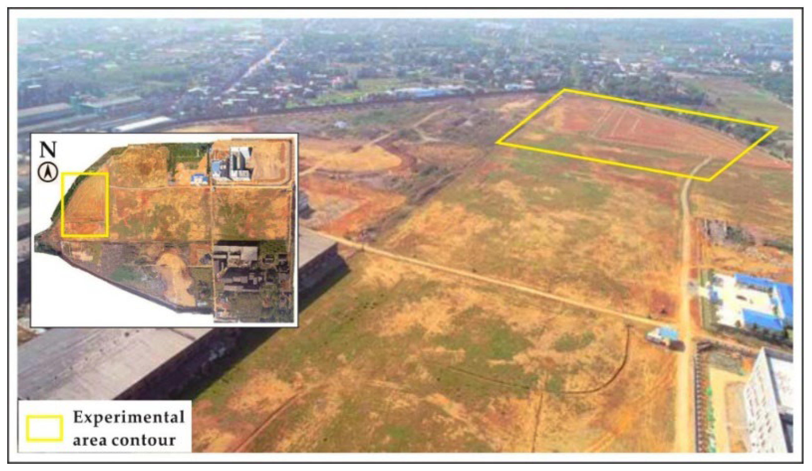
2.1. Study Area

The site selected for this study is an urban site of a former ferroalloy factory built in September 1958 and standby all factory operation in 2006. Hexavalent Chromium pollutes the soil and groundwater in the surrounding area with a maximum concentration of about 1000 mg/L. In Figure 1, the study area extension forms 450 m by 270 m long. Groundwater flow modeling is needed to be able to conduct a further numerical simulation of groundwater contaminant transport. The geological borehole data from the geological investigation shows that the area comprises miscellaneous fill, silty clay, medium silty gravel, weathered mudstone, and moderately weathered mudstone. The miscellaneous fill is highly porous, while the silty clay layer is relatively water-resisting with poor water permeability. The gravel layer is the principal confined aquifer with medium porosity, and the base is composed of the less permeable mudstone layer. The groundwater flow direction is northwest to southeast.

2.2. Datasets

The simulation data are composed of various interdependent data for each simulation step. The three-dimensional geological model data originated from exploration data, especially from 8 cross-sections and 37 additional boreholes data where the aquifer’s top and bottom elevations were used for this research (

Table 1. Utilized data for this work.

Modeling Phases	Geological Modeling	Conceptual Modeling	Groundwater Flow Simulation
Data	8 cross-sections, 37 borehole data	Surface data, GIS data (.shp) topographic data, borehole data	Observation wells data, laboratory experiment results, pumping test results

). The hydrogeological parameter data (initial hydraulic conductivity, specific storage, specific yield, and porosity) were obtained from the pumping test experiment. The laboratory testing of soil and water samples from the study area was conducted conjointly by another research group. Several methods could be used to obtain an initial hydraulic conductivity for pumping test data, such as the graphical method [20] or the type curve method [21]. The observation data comprises 37 observation wells dispersed into the model area; the hydraulic head from the study area observation value was obtained from the borehole survey screen localized at the 44 m elevation conducted during a previous hydrogeological investigation.

2.3. Preprocessing

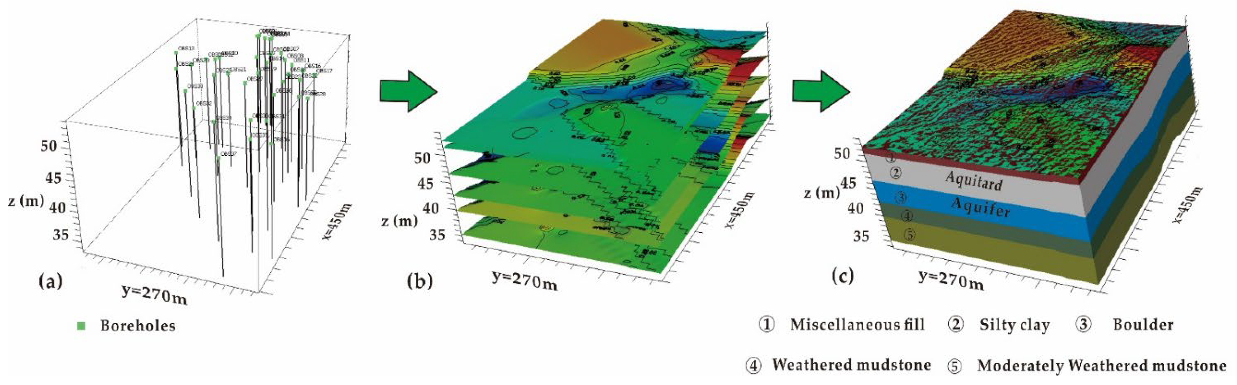
2.3.1. Geological Modeling

The three-dimensional geological model reproduces subsurface formations and their accompanying features. Several previous researches have been illustrated for three-dimensional geological modeling [22]. The experimental simulations have been conducted to approach the testing of the conversion of the three-dimension SGrid model designed from GOCAD into a processing model such as Flac3d [18], and Groundwater modeling system (GMS) transferred as a semi-regular grid using the ASCII format [23] or TIN format [24]. These studies show the feasibility of the transfer from the three-dimensional SGrid model into the three-dimensional hydrogeological model. The geological model was obtained from a GOCAD software design based on a cross-section interpolated into the TIN format [25]. The 3D SGrid model was transferred to the visual MODFLOW by conserving the structure in point structure necessary for constructing the surface of the 3D grid of the hydrogeological model.

2.3.2. Conceptual Modeling

The resolution of the partial differential equation requires a specific numerical method such as the finite difference used by MODFLOW, the finite element used by the FEFLOW, the Voronoy grid, the unstructured grid, and the arbitrary irregular polygon solution based on the Multipoint approximation flux (MPFA) [26]. The finite difference method is the most effective and stable for numerical groundwater flow [27]. A finite-difference grid is used for the present study as a solution system for the conceptual model. The grid elevation is defined from surface data interpolated using the point data elevation. The exemplary data elevation determines and reinforces a varying layer elevation (Figure 2). Surfaces could be obtained from data objects imported from Golden Surfer Software (.GRD, ESRI.ASI, DEM) [28] or from surfaces created through interpolating XYZ points of excel file from the Gocad geological model and borehole data (Figure 2a). MODFLOW fits their grid according to the horizon or the surface elevation (Figure 2b). The conceptualization includes the grid refinement as well as model parameterization. Several alternative models are considered for groundwater model conceptualization when using MODFLOW [29]. Therefore, the uncertainty caused by the conceptualization affecting the groundwater flow simulation is non-negligible and worth assessing [30].

2.3.3. Model Parameterization

Parameterization in the context of numerical prediction is a method of assigning the hydrogeological parameters of the model to represent the actual condition of the aquifer [31]. It significantly influences the model’s outcome and could be a source of uncertainty when input data is inaccurate or not specific to the model area. Parameterization is a crucial step in groundwater flow simulation. It forms the basis of the hydrogeological setting. The area of interest is a small-scale area of 450 m by 270 m large discretized into a regular grid of 54 rows by 84 columns to keep the cell size at 5 m. Hydraulic conductivity (K) range from 4.71 × 10⁻⁵ to 5.625 × 10⁻⁵ m/day for the aquifer and 7.19 × 10⁻⁸ to 8.25 × 10⁻⁸ m/day for the aquitard. The area is subject to replenishment from pluviometry over 2483 mm per year. The infiltration coefficient is about 0.1 making its input of 248.3 mm/year uniform over the whole area and the evapotranspiration of 128 mm/year.

The present study area presents the same pattern as Meijia Zhu in 2019, suggesting that lateral recharge is negligible compared to the surface recharge from the precipitation with the influence of extraction downstream [32,33]. The study area is influenced by a large river one kilometer downstream, while the groundwater follows the SE-NW direction toward the river. The east and west side of the model is a no-flow boundary. The north and south are a constant head boundary (Figure 3). According to a prior hydrogeological survey report, the specific storage is 4.9 × 10⁻⁵ m⁻¹, and the specific yield is 0.13–0.40. The high fluctuation area of the hydraulic head is fixed as a constant head along the south and north boundary condition. The median value of the boundary conditions is interpolated. The visual MODFLOW offers the opportunities to interpolate different values in every part of a linear boundary condition. The northwest part of the model represents the downgradient, and the southeast forms the up gradient. The permeability coefficients in the X and Y directions are the same, and the permeability coefficient in the Z direction is taken as 10 percent of the horizontal permeability coefficient [34].

2.4. Groundwater Flow Simulation

Groundwater models, also known as groundwater flow simulation models, are used to forecast the consequences of hydrological changes on the behavior of the aquifer [4]. Aspects of groundwater quality are included in specific groundwater models in other studies [35]. Groundwater models are employed in a variety of urban water management programs. Some groundwater models attempt to forecast the chemical’s fate and movement in natural, urban, and speculative scenarios [36]. Three-dimensional groundwater flow is based on the governing equation of groundwater based on Darcy’s law represented by the partial differential equation written in Sepulveda 2015 [37] as Equation (1).

$$\frac{\partial }{\partial x}\left(K_{xx}\frac{\partial h}{\partial x}\right)+\frac{\partial }{\partial y}\left(K_{yy}\frac{\partial h}{\partial y}\right)+\frac{\partial }{\partial y}\left(K_{zz}\frac{\partial h}{\partial z}\right)-W=\left(S_c\right)\frac{\partial h}{\partial t},$$

(1)

where x, y, and z are the permeability direction on horizontal dimension, t is the time, h is the hydraulic head, K represents the hydraulic conductivity, W is the sink term, and S_c is the storage.

Hydraulic heads for one stress period were simulated by the interface of the Layer-Property Flow package (LPF) on a steady-state condition. The unsteady state simulation based on MODFLOW USGS has been investigated [38]. The model hydraulic properties were assigned using the zonation, in our case, the downgradient, and the upgradient by the graphic user interface (GUI). Manual calibration was carried out to approach the model output results. Accordingly, manual calibration was conducted to obtain the same trend of errors; it could considerably reduce the problem of local minima and approach the sought calibration parameters values. Afterwards, the mechanic calibration using the pilot point methodology could be processed. The non-linearity of the hydraulic conductivity during the computation iteration is the main challenge in calibrating the groundwater flow model in a heterogeneous medium. Whereas the standard simulation with manual calibration, the main objective is to achieve less or equal to 50% accuracy in minimum residual error. The statistical criteria are used to evaluate the model accuracy, such as root-mean squared (RMS) and R-squared. The RMS is traditionally the primary calibration measure for the groundwater flow model. The square root of the average square of the residual error represents the difference between the onsite observed value and the numerically simulated hydraulic head (Equation (2)) [39].

$$\mathrm{r}={\mathrm{h}}_0-{\mathrm{h}}_{\mathrm{s}},$$

(2)

where r is the residual, h₀ is the observed hydraulic head, and h_s is the numerically simulated.

$$\mathrm{RMS}=\sqrt{\frac{1}{2}{\displaystyle \sum }_{t=1}^n{({\mathrm{h}}_0-{\mathrm{h}}_{\mathrm{s}})}_t^2},$$

(3)

The groundwater flow and the model comparison are measured from their R-squared described by Shinichi (2013) [40] (Equation (4)).

$$R^2=\frac{{{\displaystyle \sum }}_{i=1}^n{\left( y_i-{\hat{y}}_i\right)}^2}{{{\displaystyle \sum }}_{i=1}^n{\left( y_i-{\overline{y}}_i\right)}^2},$$

(4)

where $R^2$ is the R-squared, $\hat{y}$ is the predicted value of y, and $\overline{y}$ is the mean value of y.

2.5. Model Calibration

2.5.1. Pilot Point Placement Design

Pilot Point Placement is the method of technically defining the emplacement of each pilot point in a groundwater flow model calibration. A pilot point can be placed on top of observations or between them. Wherever possible, increasing the density of the pilot point would be advantageous for the model calibration. Specific rules, such as density, dictate the placement of the pilot point. It should be more significant where there are more observations or high hydraulic head fluctuation, and the gap in the placement is not tolerated [41]. The groundwater flow model calibration was conducted using PEST numerical code based on the inverse modeling with pilot point mode. Inverse modeling could be used to characterize aquifer and aquitard [11]. The spatial distribution of the hydraulic head was resulted by running the model simulation using the parameters generated by the PEST. In this study, The pilot points method combines the zonation that separates the upgradient from the downgradient [42]. We adopt kriging interpolation to interpolate the assigned value of the pilot points to each of the model cells as it gives a better trend in subsurface data [43]. An exponential variogram was used for the entire simulation, parallel to the Gaussian. The simulation provides proper hydraulic conductivity distribution by minimizing the residual over 10 iterations. The simulation could give an unrealistic value to approximate the observation; however, the modeler makes the balance. The PEST calibration allows regularization opportunities that concede the model to produce a unique solution. The SVD regularization and Tikhonov regularization are available in the PEST suite or PEST++.

2.5.2. Regular Pilot Point Placement

Regular placement is related to the uniform distribution of pilot point locations to form a regular grid. The regularity guarantees the existence of a pilot point at a fixed distance. This pilot point placement structure is known as the ordinary placement for pilot point model calibration. The entire model is about 121,500 m²; a grid of 60 m × 60 m and 40 m × 40 m are formed respectively for the low density and high-density pilot point, giving 35 parameters for the low density and 60 for the high. Pilot points are placed regularly in the middle of each grid which is diverse from the finite-difference grid, such as each 3600 m² have one arbitrary point for the low density and 1600 m² for the high density of pilot points (Figure 4a–c).

2.5.3. Middle Head Measurement Down Gradient Pilot Points Placement

MHMDG is a pilot point placement concept that considers the head observation measurement and the hydraulic gradient. When using the kriging method to assign the hydraulic conductivity of every cell interpolated from the pilot point, the emplacement of the pilot point must be carefully considered. The assignment of the pilot point value is completed using the zonation technique. The area is divided into upgradient and downgradient zones from the southeast to the northwest. The frequency of the regular pilot point placement is maintained. However, the pilot points are placed in the middle of the head observation, and the downgradient part is more considered. The upgradient position is filled with a spared pilot point to avoid generating a gap in the interpolation (Figure 4b–d).

2.5.4. Pilot Point Placement Criteria

Placement criteria are the principle by which the pilot point localization is chosen. It must follow a technical condition to meet the requirement of the adopted methodology. Although there is no particular rule for the pilot point placement, criteria must be addressed to fulfill the model calibration target.

As presented in the preceding paragraph, the model is a small-scale area of 450 m × 270 m. The principle is to cover the entire study area; however, avoiding oversaturation is controlled. This study is conducted using two different pilot point placements, the regular placement, the MHMDG placement, and two other parameters density based on several criteria to achieve a minimum error and maximum accuracy (Figure 4). The number of 35 represents the lower density of the pilot point for calibration, so the distance between two pilot points is 60 m, as the model is entirely covered and has one pilot point each 3600 m² and one pilot point every 1600 m². The pilot points used here are designed in three-dimensional pilot points placed on the top surface of the aquifer layer.

3. Results

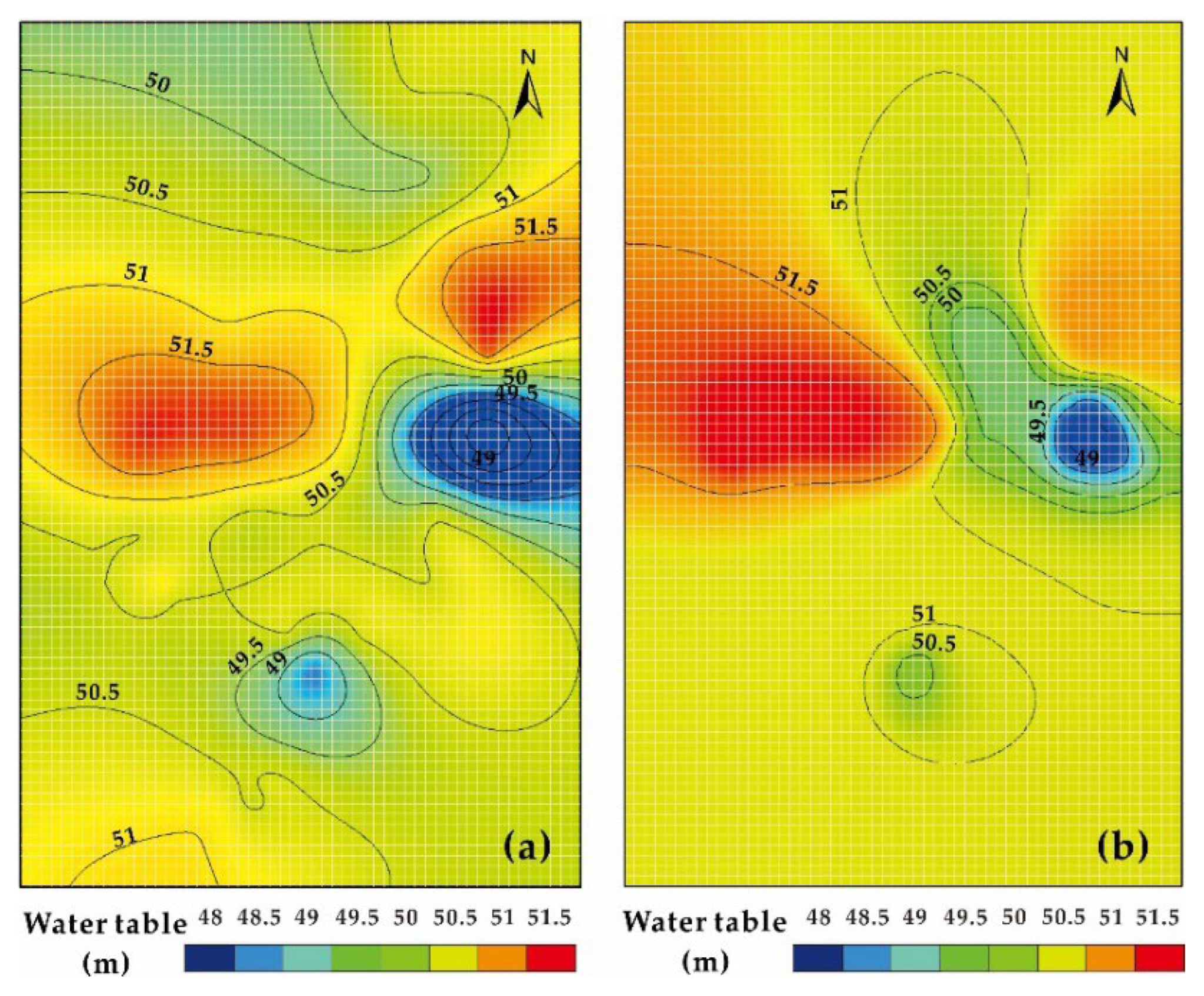
3.1. Pilot Point Placement and Frequency Effect

The pilot point placement is related to the localization of each pilot point, while the frequency is the amount of the pilot point placed in the area. The effect of these two structures could be measured by experimental simulation under various circumstances, including the convergence of the model and the measurement of the RMS. The convergence accuracy of the hydraulic head simulation reached 95% with 60 parameters, and the RMS decreased (

Table 2. Statistic of the simulation over 35 parameters and 60 parameters in regular and MHMDG pilot point placement.

Statistics	Non Calibrated	35 Points		60 Points
		Regular	MHMDG	Regular	MHMDG
Mean r squared	0.396	0.695	0.683	0.886	0.901
RMS (m)	0.69	0.38	0.34	0.37	0.32
Normalized RMS (%)	14.65	8.035	7.2	7.78	6.78
Max residual (m)	−1.6	−0.96	0.9	−1	0.9
Min residual (m)	0.078	0.0014	−0.0033	0.011	−0.0053
residual Mean (m)	−0.22	0.0063	0.024	−0.0067	0.015
Standard error of estimation (m)	0.11	0.063	0.056	0.061	0.053
K min	4.71 × 10−5	4.6 × 10−7	1.7643 × 10−7	1.7643 × 10−7	1.2867 × 10−7
K max	4.716 × 10−5	1.037081	2.445149	2.445149	0.2444386

). The middle head measurement down gradient placement takes advantage of the regular placement in terms of estimation accuracy, shown by the Standard error of estimate respectively 0.053–0.056 and 0.061–0.063.

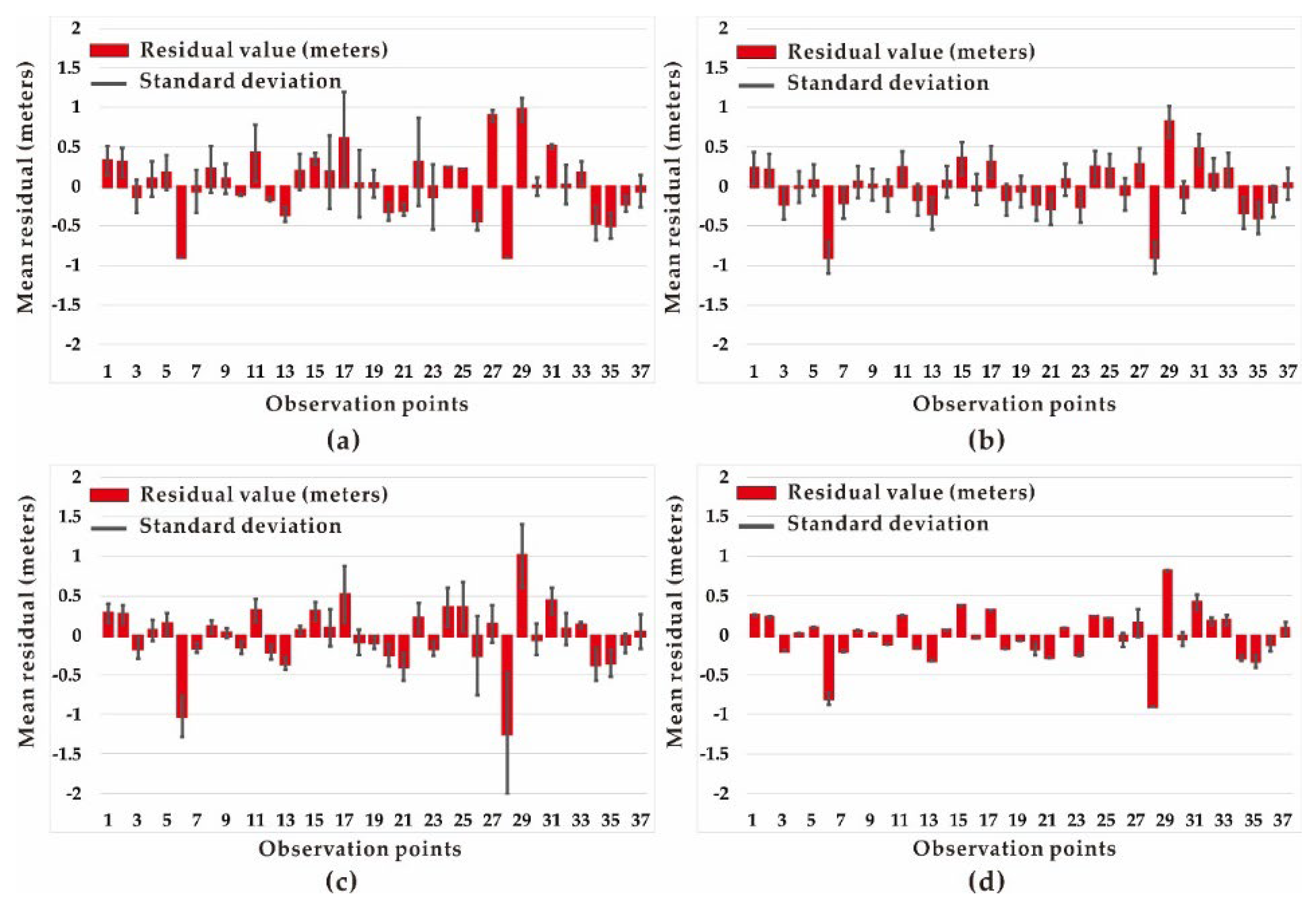
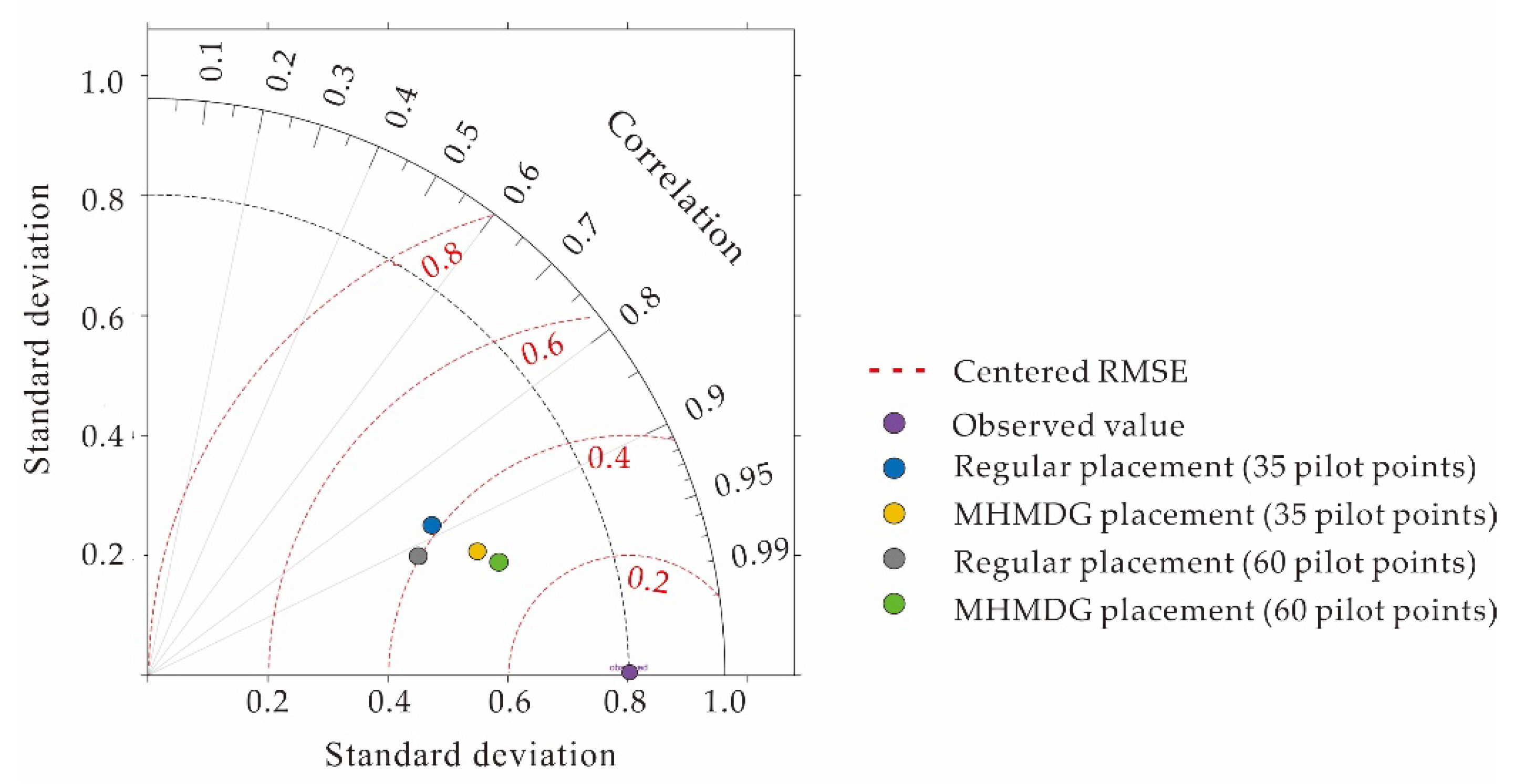
3.2. Mean Residual Error Analysis

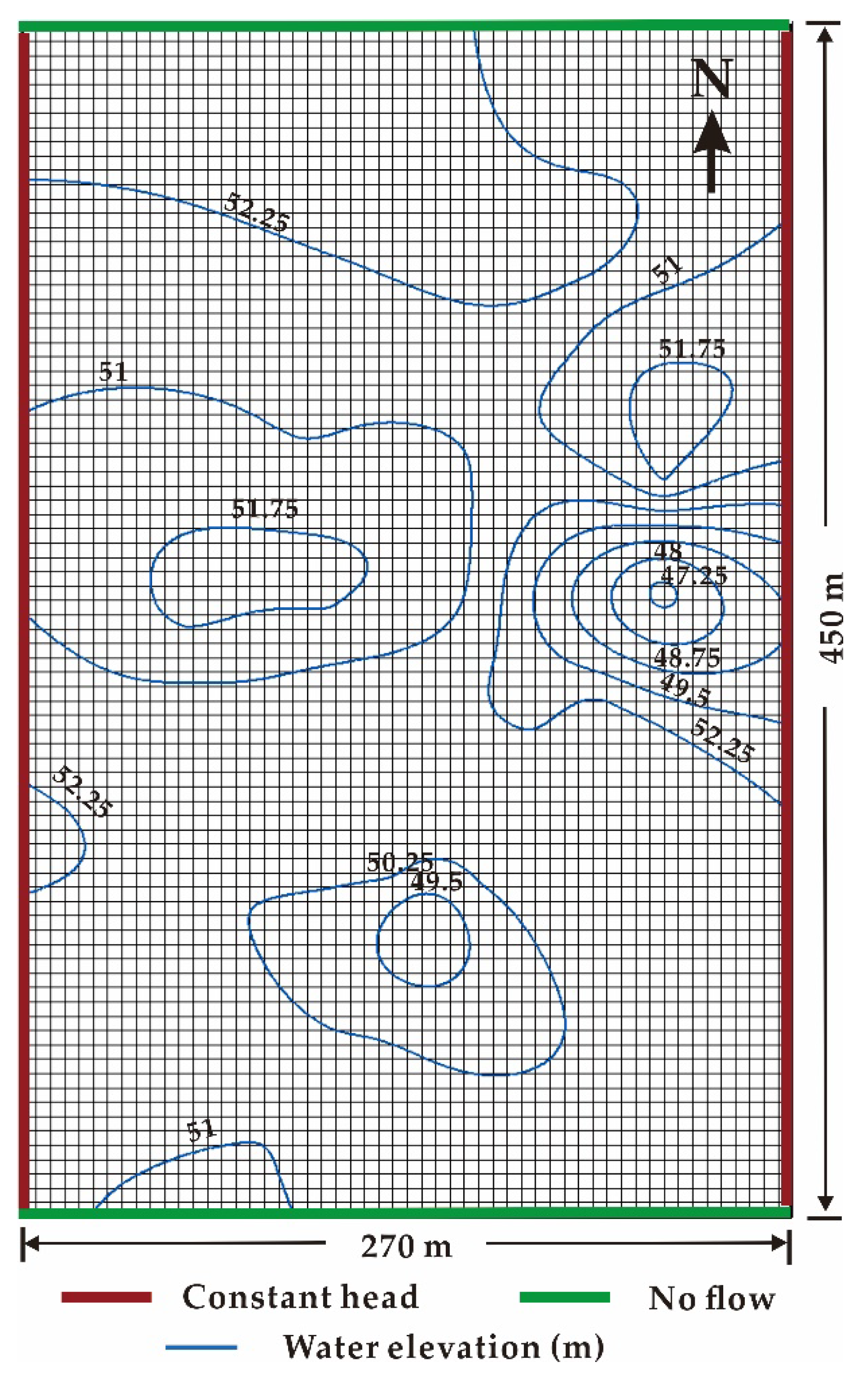
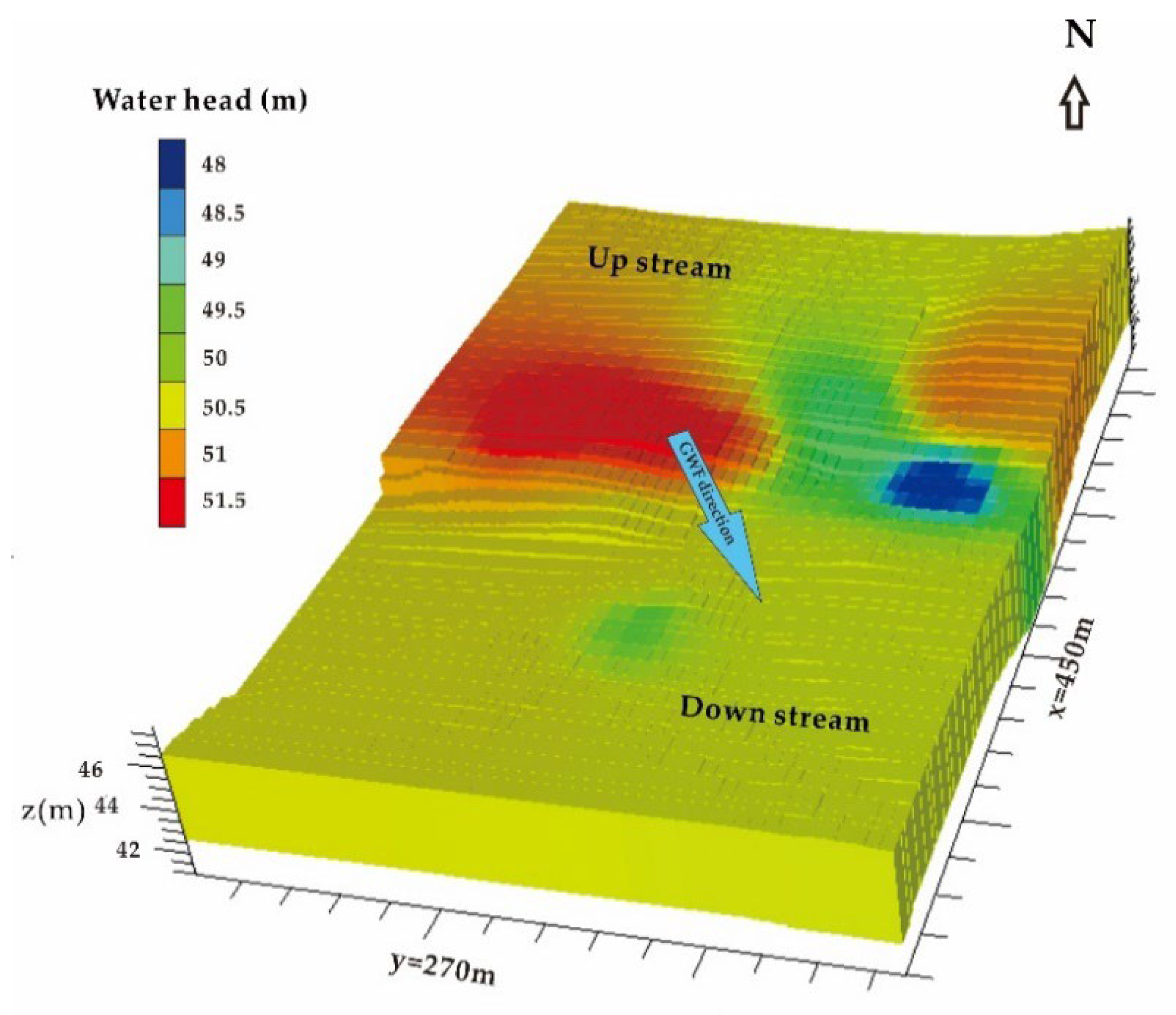
Mean residual error is the difference between the value observed and the arithmetical mean of the calculated value. It is often applied to evaluate a model or simulation [44]. Based on the number of simulations for each model design, which is ten simulations for each scenario, the mean residual is obtained and shown in Figure 5. The error bar represented here is based on the standard deviation of the ten simulation runs, which is different from the model calibration iteration. The MHMDG placement with 60 pilot points represents minor variation. The standard deviation represents a minimum value of 0 for the four types of pilot point placement. The maximum value is 0.59, 0.081, 0.77, and 0.17, respectively, for the regular placement with 35 number pilot points, regular placement with 60 number pilot points, MHMDG placement with 35 number pilot points, and MHMDG placement with 60 pilot points.

3.3. Hydraulic Head

A hydraulic head, also known as a piezometric head, is the measured water level under natural pressure [45]. The hydraulic head is one of the most critical characteristics for describing a hydraulic system’s mechanical energy condition. In the Finite-difference model, the hydraulic head is unique to every model cell as the principal groundwater flow equation solution. The confined layer, the medium silty gravel layer, is the simulation’s focus. The interpolated water table and the numerically simulated present a similar global trend with a slight difference (Figure 6). In this simulation, the hydraulic head of each cell is obtained by the calculation using the finite-difference solution in steady-state mode. The Silty clay and the medium silty gravel represent the saturated zone (Figure 7), while the confining layers are filled by dry cells.

3.4. Parameter Sensitivity Analysis

Parameter sensitivity analysis is a critical tool in result data analysis that aims to evaluate the relative importance of model parameters and identify those with a low and high impact that should be fixed or increased during analysis to keep a model stable and accurate [46]. This study applies the sensitivity analysis method described in Al-Muqdadi et al. [47]. The parameters sensitivity calculation is included in the PEST simulation, and the value is assigned to each parameter observation. The sensitivity value obtained from Equation (5) represents the influence of each parameter in the numerical simulation and the convergence of the model along the calibration iteration process.

$$S_i={\left(J^{t}QJ\right)}_{ii}^{1/2}/m,$$

(5)

where $S_i$ is the composite sensitivity for parameter i, J is the Jacobian matrix, $J^t$ is the transpose of the Jacobian matrix, m is the number of observations, and Q is the weight matrix. A similar sensitivity analysis method has been conducted for a pilot-point emplacement calibration of the karst model and applied in this main study [16]. The parameter sensitivity of the four pilot point placement settings was conducted and expressed in Figure 8.

4. Discussion

4.1. Pilot Point Based Calibration Evaluation

Through the calibration process, the estimation of the parameters gave the maximum optimized value of the hydraulic conductivity. The result shows a positive difference with a 0.901 R-squared for the 60 pilot points with MHMDG placement compared to 0.630 for the non-calibrated model when using the optimized parameters. The MHMDG 60 pilot points give a better performance than the regular placement of any density of parameters and minor change in standard deviation. Based on the Taylor theory, a concise statistical overview of the model result in terms of correlation, root-mean-square difference, and variance ratio is presented in a Taylor diagram to evaluate the model [48]. The observation and calculated values comparison show that the MHMDG placement model with 60 pilot points is the most stable and accurate calibration (Figure 9). Over the fifth iteration, the value of the parameters meets the stability conditions and the objective function. The methodology proposed here showed that the pilot-point-based calibration gives a sound approximate random output of parameters as an outcome and a close correlation between the observed data and the numerically simulated hydraulic head. The water table simulated by the MODFLOW model presents a minor variation compared to the water table interpolated from the observation data (Figure 5).

The study’s objective is to improve the technics of groundwater flow calibration based on pilot points placement through a scenario and repeated simulation experiment realized using the MODFLOW 2005 engine and the PEST suit. The frequency of pilot points influences the iteration time; the more the pilot-point density increases, the longer the computation time. However, the accuracy is increased with the density as well. The modeler must determine a balance during a manual calibration to minimize computing time and burden. The pilot point calibration method is more effective when combined with the zonation and placed between the observation wells and the boundary condition. The model simulation could not tolerate the gap of the pilot point in the model area; it must be filled with less density. With the MODFLOW 2005 engine and PEST suit, the model’s three-dimensional and two-dimensional pilot point’s influence is negligible.

In the small-scale area, the kriging interpolation with exponential variogram applied here for the assignment for the pilot point value is exceptionally suitable as it approximates the solution with high accuracy. An excessive variogram might impact the iteration and parameters sensitivity and limit the objective function, which becomes stable and constant before around 90% of the simulation. In a high water level fluctuation region, a trendier change of parameters sensibilities occurs but is less sensible in the MHMDG 60 pilot points. The other placement design’s sensitivity result does not follow any tendency (Figure 8).

4.2. Comparative Analysis

The pilot point placement results expose the applicability of the pilot point calibration methodology in the small-scale heterogeneous area focused on the estimation of hydraulic conductivity field similarly investigated in other literature [10,16,17]. The structural and stratigraphic traits and trends in these research are identical. Literature [10] emphasizes the importance of pilot point methodology for estimating transmissivity in limited field data. In contrast, the others use pilot points in surface groundwater interaction problems regarding data scarcity and combine the zonation and the pilot point method with exploring the effect of pilot point location in Karst. In addition, These works of literature emphasize the validation of the steady-state model conducted using the PEST by the database approach according to the review of the groundwater flow and calibration evaluation [4]. It has been illustrated that groundwater model calibration should be evaluated statistically prior to sufficient observation data.

Moreover, despite several methods associated with groundwater modeling, such as the artificial neural network (ANN), or the surrogate model using a genetic algorithm, the MODFLOW model takes advantage of the dynamic response of the aquifer and the application of automatic calibration [49]. The modeling using an ANN often requires extra data, such as pumping data and climate data [50]. Therefore, the MODFLOW model remains the vastly used model chosen for the present problem. These models often present an uncertainty associated with the model input parameters that could significantly impact the simulation outcome. It can be evaluated by the sensibility analysis when using the PEST for automatic calibration while needing specific technics such as full Bayesian technics [51] or Markov Chain Monte Carlo-based uncertainty analysis method [52]. However, the findings of this study could aid in focusing on areas of high uncertainty where more field data is needed to improve model calibration. It also aids in positioning pilot points for a more reliable calibration. Admittedly, the uncertainty problem could be the future development of the present situation assessed with machine learning techniques.

5. Conclusions

This paper presents an improved calibration technique for the groundwater flow model based on the pilot point method under various situations and stress circumstances. The experimental simulation is conducted using the MODFLOW model and the PEST calibration numerical code in a small-scale heterogeneous area for an MHMDG design of the pilot point method on steady-state mode. Our main findings are as follows:

(1)

The calibration evaluation compared the simulated hydraulic head to the observed data. The conceptualization method has a significant impact on the result, especially the grid structure and elevation, which define the deformation of the grid and the relief of the surface. The geological structure could be well reflected by the surface interpolated from a SGrid model elevation point. The accuracy depends on the interpolation method, which is the primary source of uncertainty. The kriging interpolation remains the most effective and accurate for groundwater model conceptualization.

(2)

The calibration method based on the pilot point method is effective in the small-scale area, as proved by this experimental study; however, it massively pivots on the pilot point emplacement strategy and density. In our application case, the MHMDG placement method with a large density gives the best R-squared 0.901 compared to 0.880 for the regular placement. The kriging interpolation used in inverse modeling reflects the value of the hydraulic conductivity of every pilot point. The initial value of the pilot points impacts the accuracy of the result and the computation time. The calculation is more complicated in heterogeneous media and generates a computation burden that affects the model stability.

(3)

The choice of the solution model and the engines adapted to the context is critical for simulation, especially when using the MODFLOW numerical code. It might yield an excellent calculation outcome of unrealistic value. The MODFLOW 2005 and the PEST combination are perfect solutions for small-scale areas. The consideration of small-scale simulation with regularization is a future topic for another research. It helps to understand the calibration solution’s uniqueness of using the pilot point method and zonation focused on the middle head measurement on the downgradient technics.

References

1. Kresic, N. Hydrogeology and Groundwater Modeling; CRC Press: Boca Raton, FL, USA, 2006. [Google Scholar]
2. Arshad, A.; Zhang, Z.; Zhang, W.; Dilawar, A. Mapping favorable groundwater potential recharge zones using a GIS-based analytical hierarchical process and probability frequency ratio model: A case study from an agro-urban region of Pakistan. Geosci. Front. 2020, 11, 1805–1819. [Google Scholar] [CrossRef]
3. Salam, M.; Cheema, M.J.M.; Zhang, W.; Hussain, S.; Khan, A.; Bilal, M.; Arshad, A.; Ali, S.; Zaman, M.A. Groundwater storage change estimation using grace satellite data in Indus basin. Big Data Water Resour. Eng. 2020, 1, 13–18. [Google Scholar] [CrossRef]
4. Zhou, Y.; Li, W. A review of regional groundwater flow modeling. Geosci. Front. 2011, 2, 205–214. [Google Scholar] [CrossRef] [Green Version]
5. Aslam, M.; Arshad, M.; Hussain, S.; Usman, M.; Zahid, M.B.; Sattar, J.; Arshad, A.; Iqbal, M.M.; Waqas, M.S. An integrated approach for estimation of van genuchten model parameters in undisturbed and unsaturated soils. Pak. J. Agric. Sci. 2021, 58, 1887–1893. [Google Scholar] [CrossRef]
6. Shoarinezhad, V.; Wieprecht, S.; Haun, S. Comparison of local and global optimization methods for calibration of a 3D morphodynamic model of a curved channel. Water 2020, 12, 1333. [Google Scholar] [CrossRef]
7. Xu, T.; Valocchi, A.J. A Bayesian approach to improved calibration and prediction of groundwater models with structural error. Water Resour. Res. 2015, 51, 9290–9311. [Google Scholar] [CrossRef]
8. Doherty, J. Ground water model calibration using pilot points and regularization. Ground Water 2003, 41, 170–177. [Google Scholar] [CrossRef]
9. Fienen, M.N.; Muffels, C.T.; Hunt, R.J. On constraining pilot point calibration with regularization in PEST. Ground Water 2009, 47, 835–844. [Google Scholar] [CrossRef]
10. Kapoor, A.; Kashyap, D. Parameterization of pilot point methodology for supplementing sparse transmissivity data. Water 2021, 13, 2082. [Google Scholar] [CrossRef]
11. Zhuang, C.; Zhou, Z.; Illman, W.A.; Wang, J. Geostatistical inverse modeling for the characterization of aquitard heterogeneity using long-term multi-extensometer data. J. Hydrol. 2019, 578, 124024. [Google Scholar] [CrossRef]
12. Giudici, M.; Colpo, F.; Ponzini, G.; Romano, E.; Parravicini, G. Calibration of groundwater recharge and hydraulic conductivity for the aquifer system beneath the city of Milan (Italy). In Impact of Human Activity on Groundwater Dynamics; IAHS-AISH: Maastricht, The Netherlands, 2001; pp. 43–50. [Google Scholar]
13. Doherty, J. Model-Independent Parameter Estimation User Manual, 5th ed.; PEST, Watermark Numerical Computing: Brisbane, Australia, 2010; Volume 268.
14. Jarray, H.; Zammouri, M.; Ouessar, M. Assessment of groundwater salinization using PEST and sensitivity analysis: Case of Zeuss-Koutine and Mio-Plio-Quaternary aquifers. Arab. J. Geosci. 2020, 13, 999. [Google Scholar] [CrossRef]
15. González-Quirós, A.; Comte, J.-C. Hydrogeophysical model calibration and uncertainty analysis via full integration of PEST/PEST++ and COMSOL. Environ. Model. Softw. 2021, 145, 105183. [Google Scholar] [CrossRef]
16. Baalousha, H.M.; Fahs, M.; Ramasomanana, F.; Younes, A. Effect of pilot-points location on model calibration: Application to the northern karst aquifer of Qatar. Water 2019, 11, 679. [Google Scholar] [CrossRef] [Green Version]
17. Tziatzios, G.; Sidiropoulos, P.; Vasiliades, L.; Lyra, A.; Mylopoulos, N.; Loukas, A. The use of the pilot points method on groundwater modelling for a degraded aquifer with limited field data: The case of Lake Karla aquifer. Water Supply 2021, 21, 2633–2645. [Google Scholar] [CrossRef]
18. Ni, X.D.; Chen, K. Study on the conversion of GOCAD models to FLAC3D models. Appl. Mech. Mater. 2014, 501–504, 2527–2531. [Google Scholar] [CrossRef]
19. Harbaugh, A.W. MODFLOW-2005, the U.S. Geological Survey Modular Ground-Water Model—The Ground-Water Flow Process; U.S. Geological Survey: Reston, VA, USA, 2005.
20. Zhuang, C.; Zhou, Z.; Zhan, H.; Wang, J.; Li, Y.; Dou, Z. New graphical methods for estimating aquifer hydraulic parameters using pumping tests with exponentially decreasing rates. Hydrol. Process. 2019, 33, 2314–2322. [Google Scholar] [CrossRef]
21. Zhuang, C.; Li, Y.; Zhou, Z.; Illman, W.A.; Dou, Z.; Wang, J.; Yan, L. A Type-curve method for the analysis of pumping tests with piecewise-linear pumping rates. Ground Water 2020, 58, 788–798. [Google Scholar] [CrossRef]
22. Yongcheng, L.; Naiqi, S.; Biao, L.; Yan, Y.; Mei, D. Research on 3D geological modeling by using GOCAD software. In Proceedings of the 2010 Second World Congress on Software Engineering, Wuhan, China, 19–20 December 2010; pp. 259–263. [Google Scholar]
23. Ross, M.; Aitssi, L.; Martel, R.; Parent, M. From geological to groundwater flow models: An example of inter-operability for semi-regular grids. Geol. Surv. Can. Open File 2006, 5048, 67–70. [Google Scholar] [CrossRef]
24. Watson, C.; Richardson, J.; Wood, B.; Jackson, C.; Hughes, A. Improving geological and process model integration through TIN to 3D grid conversion. Comput. Geosci. 2015, 82, 45–54. [Google Scholar] [CrossRef] [Green Version]
25. Witter, J.B. GOCAD® mining suite software as a tool for improved geothermal exploration. In Proceedings of the World Geothermal Congress, Melbourne, Australia, 16–24 April 2015. [Google Scholar]
26. Gao, Y.; Du, E.; Yi, S.; Han, Y.; Zheng, C. An improved numerical model for groundwater flow simulation with MPFA method on arbitrary polygon grids. J. Hydrol. 2021, 606, 127399. [Google Scholar] [CrossRef]
27. Al-Hashmi, S.; Gunawardhana, L.; Sana, A.; Baawain, M. A numerical groundwater flow model of wadi SAMAIL catchment using MODFLOW software. Int. J. GEOMATE 2020, 18, 30–36. [Google Scholar] [CrossRef]
28. Golden Software, Inc. Golden Software. Available online: https://www.goldensoftware.com (accessed on 15 November 2020).
29. Zhou, Y.; Herath, H.M.P.S.D. Geoscience frontiers evaluation of alternative conceptual models for groundwater modelling. Geosci. Front. 2017, 8, 437–443. [Google Scholar] [CrossRef] [Green Version]
30. Rojas, R.; Feyen, L.; Batelaan, O.; Dassargues, A. On the value of conditioning data to reduce conceptual model uncertainty in groundwater modeling. Water Resour. Res. 2010, 46, 1–20. [Google Scholar] [CrossRef]
31. Cui, T.; Sreekanth, J.; Pickett, T.; Rassam, D.; Gilfedder, M.; Barrett, D. Impact of model parameterization on predictive uncertainty of regional groundwater models in the context of environmental impact assessment. Environ. Impact Assess. Rev. 2021, 90, 106620. [Google Scholar] [CrossRef]
32. Knox, R.C. Spatial moment analysis for mass balance calculations and tracking movement of a subsurface hydrocarbon mound. Ground Water Monit. Remediat. 1993, 13, 139–147. [Google Scholar] [CrossRef]
33. Zhu, M.; Wang, S.; Kong, X.; Zheng, W.; Feng, W.; Zhang, X.; Yuan, R.; Song, X.; Sprenger, M. Interaction of surface water and groundwater influenced by groundwater over-extraction, waste water discharge and water transfer in Xiong’an New Area, China. Water 2019, 11, 539. [Google Scholar] [CrossRef] [Green Version]
34. He, Y.; Hu, G.; Zhang, Z.; Lou, W.; Zou, Y.; Li, X.; Zhang, K. Experimental study and numerical simulation on the migration and transformation mechanism of Cr(Ⅵ) in contaminated site. Rock Soil Mech. 2022, 43. [Google Scholar] [CrossRef]
35. Rahnama, M.B.; Zamzam, A. Quantitative and qualitative simulation of groundwater by mathematical models in Rafsanjan aquifer using MODFLOW and MT3DMS. Arab. J. Geosci. 2013, 6, 901–912. [Google Scholar] [CrossRef]
36. Locatelli, L.; Binning, P.J.; Sanchez-Vila, X.; Søndergaard, G.L.; Rosenberg, L.; Bjerg, P.L. A simple contaminant fate and transport modelling tool for management and risk assessment of groundwater pollution from contaminated sites. J. Contam. Hydrol. 2019, 221, 35–49. [Google Scholar] [CrossRef]
37. Sepúlveda, N.; Doherty, J. Uncertainty analysis of a groundwater flow model in east-central Florida. Ground Water 2015, 53, 464–474. [Google Scholar] [CrossRef]
38. Mani, S.K.; Singh, S.K.; Pandey, S.N.; Pachauri, A.K. Numerical modelling of flow towards a well in a two layer aquifer. ISH J. Hydraul. Eng. 1999, 5, 68–76. [Google Scholar] [CrossRef]
39. Khan, U.; Faheem, H.; Jiang, Z.; Wajid, M.; Younas, M.; Zhang, B. Integrating a GIS-based multi-influence factors model with hydro-geophysical exploration for groundwater potential and hydrogeological assessment: A case study in the Karak Watershed, Northern Pakistan. Water 2021, 13, 1255. [Google Scholar] [CrossRef]
40. Nakagawa, S.; Schielzeth, H. A general and simple method for obtainingR2from generalized linear mixed-effects models. Methods Ecol. Evol. 2012, 4, 133–142. [Google Scholar] [CrossRef]
41. RamaRao, B.S.; Lavenue, A.M.; De Marsily, G.; Marietta, M.G. Pilot point methodology for automated calibration of an ensemble of conditionally simulated transmissivity fields: 1. Theory and computational experiments. Water Resour. Res. 1995, 31, 475–493. [Google Scholar] [CrossRef]
42. Doherty, J.E.; Fienen, M.N.; Hunt, R.J. Approaches to Highly Parameterized Inversion: Pilot-Point Theory, Guidelines, and Research Directions; U.S. Geological Survey Scientific Investigations Report 2010–5168; U.S. Geological Survey: Reston, VA, USA, 2010; 38p.
43. Bamisaiye, O.A. Subsurface mapping: Selection of best interpolation method for borehole data analysis. Spat. Inf. Res. 2018, 26, 261–269. [Google Scholar] [CrossRef]
44. Jones, J.P.; Sudicky, E.A.; McLaren, R.G. Application of a fully-integrated surface-subsurface flow model at the watershed-scale: A case study. Water Resour. Res. 2008, 44, 1–13. [Google Scholar] [CrossRef]
45. Bear, J. Dynamics of Fluids in Porous Media; Courier Corporation: Dover, DE, USA, 1988. [Google Scholar]
46. Greskowiak, J.; Prommer, H.; Liu, C.; Post, V.E.A.; Ma, R.; Zheng, C.; Zachara, J.M. Comparison of parameter sensitivities between a laboratory and field-scale model of uranium transport in a dual domain, distributed rate reactive system. Water Resour. Res. 2010, 46, 1–13. [Google Scholar] [CrossRef]
47. Al-Muqdadi, S.W.H.; Abo, R.; Khattab, M.O.; Abdulhussein, F.M. Groundwater flow-modeling and sensitivity analysis in a hyper arid region. Water 2020, 12, 2131. [Google Scholar] [CrossRef]
48. Taylor, K.E. Summarizing multiple aspects of model performance in a single diagram. J. Geophys. Res. Atmos. 2001, 106, 7183–7192. [Google Scholar] [CrossRef]
49. Zeydalinejad, N. Artificial neural networks vis-à-vis MODFLOW in the simulation of groundwater: A review. Model. Earth Syst. Environ. 2022, 1–22. [Google Scholar] [CrossRef]
50. Coppola, E.; Poulton, M.; Charles, E.; Dustman, J.; Szidarovszky, F. Application of artificial neural networks to complex groundwater management problems. Nonrenewable Resour. 2003, 12, 303–320. [Google Scholar] [CrossRef]
51. Mustafa, S.M.T.; Nossent, J.; Ghysels, G.; Huysmans, M. Integrated bayesian multi-model approach to quantify input, parameter and conceptual model structure uncertainty in groundwater modeling. Environ. Model. Softw. 2020, 126, 104654. [Google Scholar] [CrossRef]
52. Hassan, A.E.; Bekhit, H.M.; Chapman, J.B. Using Markov Chain Monte Carlo to quantify parameter uncertainty and its effect on predictions of a groundwater flow model. Environ. Model. Softw. 2009, 24, 749–763. [Google Scholar] [CrossRef]
Figure 1. Location map of the study area.
Applsci 12 04648 g001
Figure 2. Conceptual modeling design: (a) borehole and cross-sections elevation point; (b) surface obtained from interpolation of the point data; (c) Solid geostratigraphical model obtained from the surface (z exaggeration = 10 times).
Applsci 12 04648 g002
Figure 3. Discretization using a regular grid.
Applsci 12 04648 g003
Figure 4. Pilot points placement design: (a) regular placement with 35 pilot points; (b) MHMDG placement with 35 pilot points; (c) regular placement with 60 pilot points; (d) MHMDG placement with 60 pilot points.
Applsci 12 04648 g004
Figure 5. Mean residual of the four designs of pilot point emplacement over the ten iterations: (a) regular placement with 35 pilot points; (b) MHMDG placement with 35 pilot points; (c) regular placement with 60 pilot points; (d) MHMDG placement with 60 pilot points.
Applsci 12 04648 g005
Figure 6. Water table distribution comparison: (a) Interpolated water table; (b) simulated water table.
Applsci 12 04648 g006
Figure 7. Hydraulic head distribution of the aquifer using the MHMDG 60 points placement calibration (z exaggeration = 10 times).
Applsci 12 04648 g007
Figure 8. Parameters sensitivity results: (a) regular placement with 35 pilot points; (b) MHMDG placement with 35 pilot points; (c) regular placement with 60 pilot points; (d) MHMDG placement with 60 pilot points.
Applsci 12 04648 g008
Figure 9. Taylor diagram of the comparison between the observed head and the calculated head.
Applsci 12 04648 g009