Experimental Investigation of Azimuth- and Sensor-Based Control Strategies for a PV Solar Tracking Application

Abstract

Today, the world continuously investigates the promising potential of advanced and optimized technologies for harvesting green renewable energy sources, such as a solar tracking system (STS). This study presents an actual implementation of a single-axis solar tracking system (SAST), where an azimuth control scheme is developed to precisely follow the sun’s orientation. This is demonstrated by computing in real-time the optimal azimuth angle based on the actual altitude, date, and time using an embedded microcontroller. At the same time, experimental comparisons using the azimuth-based control method compared with the proportional, integral, derivative (PID) control scheme and fixed-tilt PV systems (FTPV) are derived. Experimental results show that the developed azimuth solar tracker can autonomously follow the sun’s orientation primarily from time and location-based information and independent from the actual solar irradiance. Nevertheless, the electrical energies gained from all three tested systems revealed that using the sensor-based STS would increase the net energy production by 12.68% compared to the azimuth-based SAST, with an energy production increase of 7.7%. In addition, energy consumption by the azimuth-based STS is 65% greater than the energy consumption of a sensor-based STS due to the continuous movements of the tracker, regardless of the increase or change in power production within short periods.

1. Introduction

Many researchers from all around the world have increased their focus on renewable energy production. Solar photovoltaic (PV) systems are among the most promising renewable energy sources for generating electricity and the fastest-growing technology for improving PV energy conversion efficiency from existing solar energy [1]. Efforts are being made to effectively collect and transform a small amount of the sun’s daily heat and light to address the fast-approaching energy resource shortage problem [2]. Solar energy conversion efficiency is low; for example, conventional solar panels have a conversion efficiency of less than 40% [3]. The fact that the sunbeam frequently changes direction seasonally [4] is one of the significant contributors to this low efficiency. As a result, improving the total system energy efficiency from solar radiation using a robust solar tracking system is a widely discussed topic.

Photovoltaic panels are generally installed at a fixed angle to the country’s latitude. Seasonally, the module’s direction is manually shifted towards the sun [5] if feasible. A photovoltaic system ought to be perpendicular to the beam of light to produce maximum power [6,7]. A tracking system that preserves the panel’s perpendicular orientation with the beam of light [8] is an approach to maximizing the output energy. Solar tracking is a mechanism designed to track the sun’s movement to boost energy production by 30% to 60% over fixed installed PV systems [9,10]. To track the sun effectively, numerous concepts and methodologies have been presented [11]. This necessitates complex mathematical calculations and precise observations of many solar energy characteristics. The basic parameters in the solar energy field are solar irradiance, Greenwich Time, and Solar Time [12,13,14]. Several factors should be estimated or quantified to identify PV modules’ appropriate azimuth and alignment [15].

Based on control strategies, solar tracking systems can be classified into active and passive types [16]. Microprocessors are used in active tracking systems to control the movement of panels via motors and gears [17]. The sun’s temperature is used to heat a liquid and inflate it into gas in passive solar tracking devices. The thicker fluid can be pushed to the shaded container, shifting the weight to that side, providing a pressure gradient that allows movement and rotation [18]. The number of axes required to move the photovoltaic panels horizontally, vertically, or perhaps both dictates the system’s sophistication. Single-axis tracking (SAT) and dual-axis tracking (DAT) are the two major types [19,20,21]. In each design, mechanical drives can be used as linear actuators, gearboxes, and DC motors [22].

A single-axis tracking (SAT) system has a single axis around which the panel can be rotated to align it orthogonal to the sun’s rays. The north meridian axis is the best alignment [23]. Based on optimal angle estimates, [24] suggested a discrete single-axis solar tracker that actuates just three times each day. Experiments revealed that this tracking system provided roughly 90–94% of the solar energy produced by a similar continuous solar tracking system. Some of the single-axis tracking system designs (SAT) are vertically aligned, horizontal aligned, horizontal with inclined units, and polar aligned. In comparison to dual-axis trackers (DATs), single-axis trackers (SATs) are less expensive and less complex, but they are less efficient [25,26].

An SAT produces more than 20% of the average power of a fixed panel. The mechanical movement of a basic SAT solar module is controlled by a PIC microcontroller depending on the specified location of the sun [27,28]. Kamala et al. [29] devised an SAT system controlled by a PIC microcontroller to achieve maximum production. Dian et al. [29] conceived and designed a GPS-based sun-tracker system that allows the vertical solar tracker to follow the sun’s azimuth angle. They analyzed the performance of two solar panels that were positioned differently. The panel with SAT yielded around 22% more than the fixed PV panel in terms of average output power. In Central Vietnam, in [30], 250 W PV modules connected to the grid were adopted to test the effectiveness of an SAT solar tracking system. The experiments revealed that the tracking system consumed around 2–8% of the power produced.

In addition to the solar tracker’s configuration, the climate condition and geographical position affect the performance tracker. Even though the tracking system has the potential to increase the amount of energy gained by PV modules in many conditions, other studies suggest that it is not suitable for hot climates [31]. As a result, a thorough examination should be conducted before using the solar tracking system in any locality.

An extended study across a broad region and many countries is required to fully comprehend the energy gained by the solar tracking system on a global scale. Thus, the experimental study presented in this paper explores the actual development and implementation of an STS, where the electrical performance of different sensor- and azimuth-based control schemes was investigated. First, a numerical model of the azimuth-based STS is derived. Then, a closed-loop LDR-based control scheme is highlighted. Therefore, the presented research effort adds to the body of knowledge on quantitative analysis and detailed comparison of generated, consumed, and net power of different tested SAT systems in a high solar irradiance region of Dammam, Saudi Arabia.

2. Materials and Methods

The power produced/consumed via each tracking system was measured, investigated, and analyzed. This study was performed at Imam Abdulrahman Bin Faisal University (IAU), Dammam city, where the experimental data were further analyzed and presented. The study started by designing and fabricating the mechanical model for the SAST, then installing the needed electrical connections and components for it, and finally applying the azimuth-based and sensor-based controllers for the system to facilitate its movement correctly. Both SASTs were compared to each other to study the feasibility of these solar tracking systems in the Arab Gulf region in a harsh environment.

2.1. Mechanical Design

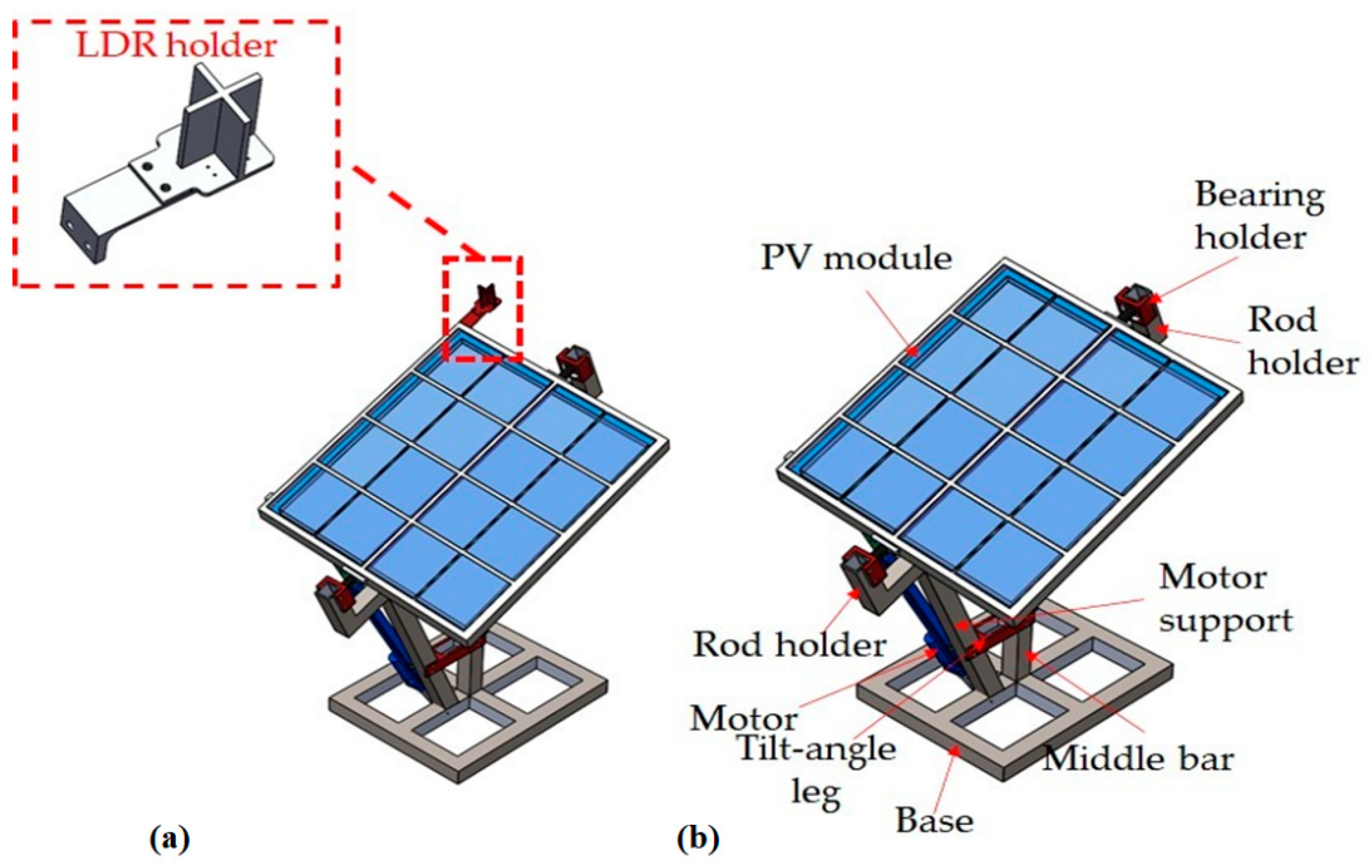
The mechanical design of the SASTs was designed using computer-aided design (CAD) software that is SOLIDWORKS, as shown in Figure 1. The SAST was designed to have a degree of freedom ranging between 60° and −60° (east (E)–west (W) direction) to follow the sun’s movement throughout the day. The assemblies were aimed to be stable under different weather conditions to obtain accurate data. Furthermore, the actual fabrication of the SASTs was carried out at the IAU FabLab and workshop, where all the needed materials and equipment were available.

2.2. Numerical Model for Azimuth-Based SAST

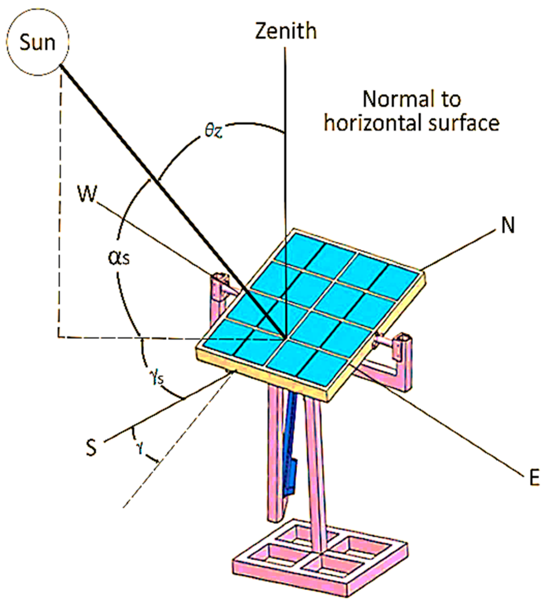
To calculate the solar azimuth angle, which is the angular distance between the south and the ground projection of the line of sight to the sun as seen in Figure 2, Equation (1) can be used. Additionally, the position east of south is signified by a positive solar azimuth angle, while a negative azimuth angle indicates a position west of south.

$${\gamma }_s=\sec ({\alpha }_s)\cos \left(\delta \right)\sin \left(\omega \right)$$

(1)

where ${\gamma }_s$ is the solar azimuth angle, ${\alpha }_s$ is the altitude angle, $\delta$ is the declination angle, and $\omega$ is the hour angle.

The altitude angle shows the height of the sun in the sky. The angle is calculated by measuring the distance between an imaginary line between the observer and the sun and the horizontal plane on which the observer stands. When the sun sets below the horizon, the altitude angle becomes negative. The altitude angle can be calculated using Equation (2) below,

$${\alpha }_s=90-{\theta }_z$$

(2)

where ${\alpha }_s$ is the altitude angle, and ${\theta }_z$ the zenith angle. The azimuth angle is the compass direction from which the sunlight is coming. At solar noon, the sun is always directly south in the Northern Hemisphere and directly north in the Southern Hemisphere. At the equinoxes, the sun rises directly east and sets directly west regardless of the latitude, thus making the azimuth angles 90° at sunrise and 270° at sunset. The zenith angle can be calculated using Equation (3).

$$\cos ({\theta }_z)=\cos \left(\varphi \right)\cos \left(\delta \right)\cos \left(\omega \right)+\sin \left(\varphi \right)\sin \left(\delta \right)$$

(3)

where ${\theta }_z$ is the zenith angle, $\varphi$ is the latitude, $\delta$ is the declination angle, and $\omega$ is the hour angle. The latitude is the angle formed by the radial line connecting the place to the center of the earth with the projection of the line on the equatorial plane as a point or location. At 90° latitude (North Pole) and −90° latitude (South Pole), the earth’s axis of rotation contacts the earth’s surface (South Pole). Therefore, the intersection of a longitude and a latitude angle may be used to designate any point on the earth’s surface. The declination angle is the angular distance between the North and South Poles to the earth’s equator, and it can be calculated using Equation (4),

$$\delta =23.45\sin (360\frac{284+n}{365})$$

(4)

where $\delta$ is the declination angle, and n is the number of days in the year. The hour angle is the angular displacement of the sun east or west of the local meridian due to the rotation of the earth on its axis at 15° per hour considering Solar Time, where morning times are negative and afternoon times are positive. Because the earth’s axis is inclined by 23.34° from the plane of the earth’s orbit around the sun, the declination angle varies from 23.45° north on 21 December in winter to 23.45° south on 21 June in Summer [32].

The Solar Time parameter is highly significant since it is the actual time affected by the sun’s location in the sky. It can be calculated using the Equations (5)–(7) shown below. The fundamental basis of this time is the day order in the year, which begins on 1 January and ends with 365 on 31 December [13].

$$Solar time-Standard time=4\left(L_{st}-L_{loc}\right)+E$$

(5)

$$\begin{gathered} E=229.2 \left(0.000075+0.001868\cos B-0.032077 \sin B \\ \hspace{1em}\hspace{1em}\hspace{1em}\hspace{1em}\hspace{1em} -0.014615\cos 2B-0.04089\sin 2B \right) \end{gathered}$$

(6)

$$B=\frac{\left(n-1\right)\times 360}{365}$$

(7)

where $L_{st}$ is the standard meridian time zone, $L_{loc}$ is the location’s longitude, B is the displacement of time from the standard time, and n is the number of days in the year. Additionally, to measure the standard meridian time zone, the time difference between local standard actual clock time and Greenwich Meantime should be multiplied by 15° (e.g., the $L_{loc}$ for KSA is 45°). Longitude is an imaginary line that is around the earth from the North to the South Pole. Another name for the longitude line is the meridian, where each meridian represents the measures of one 1° east or west of the prime meridian. Another critical angle is the angle of incidence (θ), which is the angle formed by the sun’s rays falling on a surface and the perpendicular ray as seen in Figure 3, [33]. An STS is originally designed to minimize (perfect STS would make θ = 0°) incidence angle.

2.3. Electrical Setup

To facilitate the mechanical assemblies that were designed and carry out the experimental work, different electrical components were used in this study, as seen in

Table 1. The electrical component.

#	Component	Model Number	Specifications	#	Component	Model Number	Specifications
1	Current Sensor	ASC712	5 V	7	Power Resistor	JIANXIN-09-13-318-02	100 W 8 Ω
2	Motor driver	L298N	Driver Voltage: 5–35 V Driver Current: 2 A	8	Round Rocker Power on/off Switch	-	On/off toggling
3	Micro-SD card module	SDHC	5 V Micro-SD card Work on SPI communication	9	Arduino mega	-	5 V
4	Real-time clock, with 3.3 V coin battery	DS3231 (coin cell battery: CR2032)	3.3 V Last for 10 years Work on I2C Protocol	10	DC Motor Electric linear Actuator	JS-TGZ-U1	12 V DC 30 mm/s 200 N
5	Accelerometer	MPU6050	5 V Work on I2C Protocol	11	Kayen Solar Battery (12 V, 100 Ah)	RZ2018.12	12 V, 100 A
6	Humidity and temperature sensor	DHT11	5 V	12	Solar Panel (50 W max, 12 V)	TSE-12V-50Watts 2016–0114	Isc = 3.629 A, Voc = 20.209, Im = 3.290 A, Vm = 16.513, Pm = 54.333W

. Regarding the electrical component, various components have been used to measure and assess the experimental parameter aimed in the study. The systems work dependently on an external 12 V DC battery which can be charged via the sun using a solar charger controller. In addition, linear actuators that have been connected to motor drivers are used to give the movement to the STS. The motor driver can courteously receive the digital signal from the control unit chosen to be Arduino mega.

Additionally, a real-time clock module (RTC) and accelerometer were installed to give the actual time and angle to the control unit to be used in the previous equation, as seen in Figure 4. The accelerometer determines the angle of the PV module by utilizing the gravitational acceleration and depending on the angle the acceleration on the X, Y, and Z axis differs, and the angle is calculated accordingly.

$${\theta }_{actual}={\tan }^{-1}\left(\frac{X}{\sqrt{Y^2+Z^2}}\right)$$

(8)

where ${\theta }_{actual}$ is the actual angle of the PV module, $X, Y,$ and $Z$ are the accelerometer values in x, y, and z axes, respectively. On the other hand, the light-dependent resistors were used in the sensor-based STS. Current sensors were used to compare the generated and consumed power from each system. Power resistors acting as dummy resistors were connected to PV modules and the current sensors. Additionally, one current sensor was installed in the control unit to measure its consumption. Both humidity and temperature sensors were added to the setup to measure relative humidity and ambient temperature. Finally, a micro-SD card module was used to save the data.

2.4. Control Schematic

The STS system was implemented based on a PID controller tuned by a trial-and-error approach to find the desired PID gains experimentally. The gains of the PID controller were found to be optimum at kp = 150, kd = 0.5, and ki = 0.5. The functional block diagram of the systems is illustrated in Figure 5. As mentioned previously, the main objective of using an STS is to track the sun rays via changing the solar module’s tilt angle or azimuth angle as time elapses. The aim was achieved in this study by using both azimuth-based and sensing-based closed-loop algorithms.

In the azimuth-based STS, the calculated azimuth angle based on a given latitude and longitude is considered as the input to the system. At the same time, the output is the signals that are continuously sent to the motor driver. Additionally, the accelerometer is the sensing component in this closed-loop system that measures the actual angle and compares it to the desired one. On the other hand, the sensor-based STS uses light-dependent varying resistors (LDR) as a sensor and does not need any input data, where a light-dependent resistor is a photoresistor whose resistance differs according to the light intensity projected on its surface. The error signal in both systems entered the PID controller with an anti-windup mechanism to reorient the modules without any sudden or unstable movement. The saturation block aims to clip out the effort signal if it exceeds a certain threshold level to prevent any unrated input to the DC motor dynamic, which prevents the systems from any environmental factors that might affect the stability of the metallic platform setup.

The azimuth-based algorithm of the tracker is illustrated in Figure 6. As shown in Figure 6, the microcontroller starts initializing the code variables and constants for the sensors, modules, and temporary variables that are intermediate in the algorithm. After that, the accelerometer begins to read the initial orientation of the solar module to be used in later steps. Then, latitude and longitude are entered simultaneously. The real-time clock module (RTC) reads the time and date. The latitude, longitude, and time are used to calculate the azimuth angle and consider it a command signal via the previously mentioned equations. The azimuth angle is limited to be between 60° and −60°, so the input signals are supposed to be between these two values. The error will be tested if it has a value less than or equal to 0.5 to stop the algorithm. This technique will ensure that any insignificant errors within specific tolerance are eliminated.

The sensor-based algorithm is illustrated in Figure 7, where the same analogy used at the beginning of the azimuth-based algorithm is used. The only difference in this algorithm is that there is no needed input command to the system since the signals coming from the LDRs are enough to calibrate the error signal. Then again, the same as for the azimuth-based algorithm, this error would be examined if it is in the permissible error window or not, as seen in Figure 7.

3. Experimental Procedure

The investigation of the azimuth-based SAST and sensor-based SAST was carried out simultaneously on a sunny clear sky day at IAU, in Dammam city (26°26′03″ N, 50°06′11 E). The experiment was performed on 10 February 2022, from 9 a.m. until 4:30 p.m. All the systems were facing the south, since KSA is in the Northern Hemisphere with 23 degrees of yearly tit angle, and the IAU latitude is between 25° and 50° and based on Equation (8). The ambient temperature was around 22° and the relative humidity of around 42%. Figure 8 demonstrates an actual representation of the azimuth-based and sensor-based SASTs.

$${\beta }_{Yearly}=\left(\varphi \ast 0.76\right)+3.1$$

(9)

where${\beta }_{Yearly}$ is the optimal yearly tilt angle, and $\varphi$ is the latitude.

Test protocols developed from the International Electrotechnical Commission (IEC) 62,817 standard were used to evaluate solar tracking accuracy in an experimental setting. The overall mean instantaneous solar tracking error was about 0.4° with a calibrated digital solar sensor. On the other hand, the installation cost of the system with trackers for solar production is given in

Table 2. Cost of the system.

S. No.	Material Type	Property	Quantity	Cost
1	PV Panel	24 VDC, 50 W, monocrystalline	3 Pc.	USD 3500
2	Battery	12 VDC, 10 A	1 Pc.
4	Microcontroller and Sensors (LDR, accelerometer, voltage, current, and RTC)	24 VDC–220 V	Multiple
5	Linear Actuators	12 VDC–2 A	2 Pc.
6	Main Structure	Aluminum frames	20 m

. The daily average for the sun tracking system PV panel was about 9 MJ, and using the cost research analysis conducted with actual prices of 2021, the cost of the sun tracking system was estimated to be USD 3500.

4. Results and Discussion

4.1. Power

The power of the different PV systems was analyzed to determine which PV system is most suitable. The power production of the PV modules and the power consumption by the actuation mechanism must be studied, where the system with the highest net power is the more efficient system. It is expected that the sensor-based solar tracking system would have the most increased power production since it follows the sun directly. In contrast, the azimuth-based solar tracking system uses equations to operate. However, the net power of the systems to actuate is the cut-off point upon determining the efficient system, which depends on the power production and the power required from the systems to actuate.

4.2. Power Production

Figure 9 represents the power generation of the sensor-based system compared to the azimuth-based system during day hours. The power production of the sensor-based tracking system and the azimuth-based tracking system was recorded throughout the sun hours of 8 February 2022. The results show that the sensor-based PV system’s module generated higher power throughout the day than the azimuth-based PV system. The maximum power generation of the azimuth-based system was 49.7 W at 1:01 p.m. In contrast, the minimum power generation was 46.4 W at 12:47 p.m. As for the sensor-based system, the maximum power generation was 57.1 W at 11:47 a.m.

The mean power generation of the sensor-based system and the azimuth-based systems were 52.6 W and 48.8 W, respectively, whereas the sensor-based system had a higher power generation of 7.8%. The maximum difference between the systems’ power generations was 8.1 W, recorded at 11:47 a.m. On the other hand, the minimum power generation was 48.8 W at 2:43 p.m.

4.3. Power Consumption

The power consumption of the azimuth-based and sensor-based systems through the day hours is shown in Figure 10. The power consumption of the control unit, the sensor-based tracking system, and the azimuth-based tracking system was also recorded throughout the sun hours. The results showed that the azimuth-based PV system has a higher power consumption throughout the day than the sensor-based PV system. As for the power consumption of the control unit, it is fair to say that it was steady throughout the day compared to the tracking systems’ consumption. The maximum power consumption of the azimuth-based system was 6.3 W at 9:34 a.m.

In contrast, the minimum power consumption was 0.13 W at 8:52 a.m. As for the sensor-based system, the maximum power consumption was 6.0 W at 9:05 a.m. On the other hand, the minimum power consumption was 0.04 W at 2:35 p.m. The leading difference between the systems’ power consumption was 6.5 W which was recorded at 9:48 a.m., where the azimuth-based system had higher consumption. The mean power consumption of the sensor-based system and the azimuth-based systems were 1.4 W and 4.1 W, respectively, whereas the azimuth-based system had a higher power consumption of 192%.

4.4. Energy Analysis

Figure 11 represents the net power comparison of the azimuth-based system and sensor-based and system during day hours.

The net power production of the sensor-based tracking system and the azimuth-based tracking system was calculated by subtracting the power generation from the power consumption. The results show that the sensor-based PV system’s module has a higher net power generation than the azimuth-based PV system. The maximum net power generation of the sensor-based system was 56.9 W at 12:20 p.m. In contrast, the minimum net power generation was 43.8 W at 9:04 a.m. As for the azimuth-based system, the maximum net power generation was 48.6 W at 8:52 a.m. On the other hand, the minimum net power generation was 39.2 W at 12:47 p.m. The maximum difference between the systems’ net power generation was 13.2 W, which was recorded at 9:55 a.m. The mean net power of the sensor-based system and the azimuth-based systems were 51.3 W and 44.7 W, respectively, where the sensor-based system had a higher power generation of 14.8%.

Each solar tracking system’s energy generated and consumed was calculated by taking the area under the power curves vs. time to obtain the total energy generated and consumed for both systems, as shown in

Table 3. Energy generated, consumed, and net by the azimuth- and sensor-based SASTs.

System	Energy Generated (MJ)	Energy Consumed (MJ)	Net Energy Generated (MJ)
Sensor-based system	9.06	0.234	8.83
Azimuth-based system	8.41	0.670	7.71

. The higher energy generation was from the sensor-based system with a total of 9.06 MJ compared to the azimuth-based where the total energy generation was 8.41 MJ; therefore, the total energy generation of the sensor-based system was higher in comparison to the azimuth-based system by 7.7%. On the other hand, the total energy consumed by both systems was calculated by the same method to extract the energy consumed by the sensor-based and the azimuth-based systems’ actuators. The system with the higher energy consumption was the azimuth-based actuator with a total of 0.670 MJ, and as for the sensor-based system, the total energy consumption was 0.234 MJ. The azimuth-based system had a higher consumption of 65% than the sensor-based system’s energy. After that, the total net energy was calculated by subtracting the total energy consumption from the total energy generation of each system, as shown in Table 2. The total net energy generated by the sensor-based system was 12.68% higher than the azimuth-based SAST.

The results of the net power generation and the total energy of the different systems show that the sensor-based solar tracking is more effective than the azimuth-based solar tracking system and has more potential in the region where the test was carried out.

5. Conclusions

As the world seeks alternatives for fossil fuel, renewable energy in general, and solar PV energy especially, presents a bright, promising future. An STS is one of the technologies that increase the PV system production via minimizing the reflected sun rays from a PV module surface and maximizing the transmitted sun rays through a PV module surface. The current work represented an experimental investigation for azimuth-based SAST and sensor-based SAST to study the feasibility of different STSs. In this study, the design for the different STSs was presented, the actual fabrication was achieved, the control schema for each STS was applied, and the actual experimental investigation was carried out for the different STSs simultaneously. The results showed that the sensor-based STS generated 14.8% more net power than the azimuth-based STS, where the sensor-based STS produced 7.8% more power than the azimuth-based STS, and the azimuth-based STS consumed 192% more power than the sensor-based STS. Additionally, the electrical energy balance revealed that using the sensor-based STS would increase the net energy production by 12.68% compared to azimuth-based SAST, where the energy produced by the sensor-based STS was 7.7% more than the azimuth-based STS energy production. In addition, the energy consumed by the azimuth-based STS was 65% more than the consumption of the sensor-based STS. The study concluded that using the STS is still convenient in the studied area, which implies that the proposed solar tracking system can be implemented in solar system applications in Dammam. Furthermore:

• The sensor-based STS is more efficient than the azimuth-based STS, due to its low consumption and high tracking accuracy since it follows the actual rays of the sun.
• On the contrary, the azimuth-based STS is less efficient than the sensor-based STS, due to its colossal consumption and low tracing accuracy since it follows the theoretical location of the sun only.
• This study suggests examining the degradation rate of each STS, in addition to investigating the impact of different weather conditions on the STS. Moreover, the effect of designing a hybrid STS (that combines both STSs) should be carried out to understand the feasibility of using this combined STS.