Performance Analysis of a Repairable Production Line Using a Hybrid Dependability Queueing Model Based on Monte Carlo Simulation

Abstract

Due to the augmented complexity of the factory on the one hand and the increased availability of information on the other hand, nowadays it is possible to design models of production lines able to consider the state of the health of the production system. Such models must combine both the deterministic and the stochastic behaviours of a system, with the former accounting for the mechanics and physics of the industrial process and the latter for randomness, including reliability of the production systems and the unpredictability of the maintenance and of the manufacturing lines. This study proposes the application of a Hybrid Dependability Modelling based on Monte Carlo simulation to estimate the performances of a repairable production line modelled with a queueing G/G/1 system. The model proposed is characterized by random interarrival and service times and by the wearing and dynamic aging phenomena of the machine tools that depend on the working and operating conditions.

1. Introduction

Industry 4.0 is playing a crucial role in the digital transformation of manufacturing/production and related industries as it provides new paradigms for the management of the enterprises. Cyber–physical systems form the basis of Industry 4.0 (e.g., “smart machines”), and they are becoming predominant also in small and medium enterprises (SMEs), such as in several phases of the manufacturing and production processes [1].

The success of any industry is tightly interconnected to its suppliers and to the response of the market. Under this viewpoint, Industry 4.0 can represent a great opportunity to improve the effectiveness of the value chain [2] because the collaboration among the actors of the supply chain can be facilitated by the digitalization of the Smart Factories. In fact, Smart Factories become able to exchange real-time information and increase the transparency among each other [3] thanks to their advanced equipment constituted by hi-tech robotics and artificial intelligence, IoT sensors, cloud computing, data capture and analytics, digital fabrication (including 3D printing), software-as-a-service and other new marketing models.

The efficiency of a production system is, indeed, one of the main drivers of competitiveness. The quantity of different products and the uncertain demand require an increased flexibility in terms of manufacturing which, in turn, requires the ability to adapt to the market demand and supply uncertainties [4].

In the context of the SME, more flexible and less expensive tools, supported by a growing number of new technologies, are being preferred to traditional enterprise information systems, such as ERP and MES [5,6]. They can be easily integrated with modern control and embedded software systems, allow individuals to monitor and process data control via IoT (the Internet of Things) and Internet and improve the overall management and scheduling of industrial processes, from the production to the maintenance.

From the field-level of a production department, it is now possible to capture many important signals that can be collected and used to evaluate the status of the system. Moreover, the diffusion of data analytics tools is helping the organizations in the understanding of meaningful information from the produced data. Nowadays, it looks possible to code models able to capture information data of operational behaviours that link environmental conditions, workloads and cumulative aging of materials which were not available before. As highlighted by [7], systems are generally working under time-varying operating conditions that can influence the failure time of systems. In the modelling of a queueing system [8], the trivial hypothesis of a dyadic state (working, failed) is not realistic because industrial and electromechanical equipment are deteriorating from wearing and ageing effects. As discussed in [9], one of the main challenges is the unpredictability of the manufacturing lines that can be tackled with novel tools, including digital twin and simulation, of the Industry 4.0 generation.

In this context, in order to better assess the main performance and dependability attributes of the system, including reliability, availability and maintainability [10], the development looks promising in the investigation of a methodology that can combine a realistic model of a production line with up-to-date and more detailed information data of the equipment. A general dependability framework has been proposed in [11], and in this research paper, it has been modified in order to integrate it into a dynamic reliability problem [12]: a non-exponential queueing system subjected to non-exponential failure and repair and characterized by dynamic working conditions (process scheduling and workloads).

Due to the numerous physical and stochastic interdependencies typical of a multi-state system, the choice for the use of the simulation paradigm over any other mathematical formalism appears the most suitable. The simulation model is fed by the mechanical differential equations of the machine tool wearing which are integrated numerically. Moreover, the proposed simulation environment, coded within the electronic spreadsheet, can be easily interconnected (using many plugins, such as OPC-DA, Modbus, ODBC, etc.) to a production line to get real-time data from the field level (operational variables), communicate the diagnosis of its status (evaluation of aging) and control the operations (assessing its remaining useful life) as a cyber physical system.

This paper is organized as follows: In Section 2, a thorough literature review about repairable queuing systems modelling is presented in order to depict the state of the art and to identify the space of intervention. Section 3 presents the theoretical background of reliability and repairable queueing systems to better frame the concepts in place—what are their main limitations and how they can be combined in a simulation of a dynamic reliability problem. The flowchart algorithm of the Hybrid Monte Carlo simulation able to solve the challenge of a generic repairable queueing system with a dynamic reliability problem is thus presented. This represents one of the main novelties with respect to the state of the art described in the next section. With the aid of a case study, Section 4 presents the hybrid simulation model and the design of the experiment that consists of different working scenarios under a corrective maintenance policy. This latter includes, among everything else, some validation scenarios that are used to test the correctness of the simulation model. Finally, conclusions are reported in Section 5.

The proposed paper is thus providing a theoretical framework to evaluate the performance of a production line characterized by wearing and aging which can be coded according to different types of production hypotheses. Moreover, it can be coded to connect the electronic spreadsheet to a production environment and achieve more realistic information from the field, providing to the production stakeholders a powerful tool that works not just offline but also in real-time.

2. Literature Review

Production scheduling, maintenance scheduling and quality management are three shop floor level policies that aim to minimize the costs of a manufacturing business. Job rejections, machines’ down time, waste, manpower, energy, raw material and delay costs are all the consequences of a mishandled management of the production activity. Although these three policies have been treated as separate problems in the past [13], comparing the three different maintenance policies, the interdependencies between them and the competitive markets together have shifted the recent studies to analyse joint considerations for which, based on the objectives, different models are proposed [14]. In the literature, the interest of research and practitioners for finding optimal values of floor-shop variables is demonstrated by many recent papers that undertake this goal by proposing different mathematical, engineering and operative research solutions that are often conceived to solve the specific use case under investigation.

A non-linear programming approach to model a joint production and maintenance scheduling (JPMS) with multiple preventive maintenance services and determine the best sequence of jobs is proposed in [15]. The results demonstrate the effectiveness of the proposed algorithm that remains valid under the hypothesis of constant failure and repair rates. Conversely, the objective to determine the maintenance plan of deteriorating production machines subject to a production scheduling system is discussed in [16,17,18], with the main assumptions of a Markovian process. In [19], a model that includes two coupled Markovian queues is presented, with one queue that represents the decoupling inventory and the other the order backlog.

The Weibull distribution characterizes the failure behaviour of the single station problem proposed in [20] where an optimisation problem for the job scheduling with, at most, 18 items is solved, assuming preventive maintenance. As it can be seen, the resolution approach to these problems is with meta-heuristic methods, with a dependability model that is set with a well-defined probability density function of failure/repair.

Another class of problems for queueing systems deals with minimizing loss (of materials or time) either by focusing on the properties of the queue or service station. If such models are coupled with a stochastic dependability model, they can provide important key performance indexes of a production system, identifying bottlenecks and weaknesses, and other relevant hints that can reveal and improve the effectiveness of the production operations, from the production scheduling to the maintenance policies. This latter category, known as “queue with unreliable service station” or “repairable queue”, is the main focused by this manuscript.

The resolution of unreliable queues is an interdisciplinary field between queueing model, dependability and operational research. The main measures of a queueing system such as waiting time, queue length, station occupancy, etc., are the objectives of such analyses. Analytical methods, heuristic methods and simulations are the main methodologies used to model and solve this class of problems.

Analytical methods include generating function, stochastic decomposition, renewal processes and Quasi-Birth–Death (QBD) models. For instance, in [21] a mathematical model for the optimal quality and process control of a queueing production system is proposed to maximize expected profit per unit time. Unscheduled and preventive maintenance of a single unreliable station processing N jobs are analysed [22] using arguments from renewal theory which stick to a mathematical model to obtain a closed form solution. An interesting evolution of such modelling is presented by [23] which focuses on condition-based maintenance to increase the system-level performance of a degradation system described with a Markovian model. A transition matrix is used in their solutions with the limitation that this analytical model can be applied only to a few operational scenarios.

In the general category of the problem of a queue with unreliable service stations, there is a specific type of problems called repairable queues with degradation. In this case, it can be assumed that the service station can fail during the production activities either because of a fault or due to a degradation of its workload capacity. Such type of scenario is very common and difficult to analyse with a pure analytical approach. The research papers [8] adopt an analytical explicit solution for an M/M/1 of a repairable queueing model, and [24] shows an approach to model the failure rate of the service station that depends on the age of the components, without considering when the system is in idle or in a busy mode. Arrival rate of the jobs and occurrence of failures follow a Poisson process; service time and maintenance time are exponentially distributed.

The attention over the working conditions which can affect the system performance is another important setting for this type of modelling. In [25], the authors examined an M/M/1 retrial queue with an unreliable server in an exogenous random environment and obtained the approximate orbit size distribution and mean queueing performance measures using matrix–analytic methods (level dependent QBD). In addition, [26] considered a variable failure rate for a M/M/1 queueing system with repairable service station with different parameters in idle time and busy time. They used transform method (QBD) to obtain the steady-state availability and the generating function method to obtain steady-state mean queueing length. Moreover, [7,27,28] focus on a single component system: [7] assumed time-varying operational conditions that are modelled by means of a continuous-time Markov process, whereas [27] combined a continuous-time Markov chain with queueing theory to obtain a model for the optimization of the repairing costs. In another work, [29] studied the M/M/2 repairable queueing system with varying failure rate at different times and used transform method (QBD) in steady-state period to obtain the probability of the states, the steady-state availability and the steady-state queueing length. In [30], authors presented and used an analytical method based on a decomposition approach that applies to a multi-stage manufacturing system. The queueing system was modelled with a Markov process and the degradation with a fixed decreasing yield that does not depend on the physics of the system and of the manufacturing process.

As it can be noticed, the previous papers narrow the scenarios to the assumption that the distribution of failure, repair, interarrival and service are random and can be modelled with the Poisson distribution. This represents an important limitation for models which aim to analyse real production environment. Moving towards a more realistic modelling, an evolution model for the failure rate is proposed in [31] to evaluate the optimal integrated predictive maintenance strategy on the manufacturing system with a gamma process to characterize the performance degradation. Although this kind of modelling can be defined as hybrid because it combines at once mechanics and stochastic behaviours of the system, the main limitation of the previous manuscript is that the degradation follows a specific distribution, set as input of the model. A different viewpoint is presented in a recent work [32] that focuses on a joint model of production, quality control and preventive maintenance for a serial–parallel multistage production system. The complexity of the problem is higher than single stage queue and, as in [33], the novelty proposed is to evaluate the machine structure importance measure and productivity when selecting the machine to put in maintenance. In this case, the problem is modelled and solved by means of Monte Carlo simulation, but only a single quality attribute for modelling the machine deterioration is considered without taking into account the active contribution of operational conditions.

Therefore, according to the literature review performed, the main limitations addressed in this manuscript are to enable a general modelling of repairable G/G/1 queue with a repairable service station subjected to wear and aging. These, depending on the jobs scheduling, the environmental and the working conditions, will be integrated into the mechanical equations of physics for the modelling of the system dynamic failure rate. Moreover, although the working station can be in a failure or degraded state [28], the manufacturing system can, eventually, continue its work at a reduced capability and, thus, increase the number of items waiting in the queue. Therefore, to model the proposed system, a Monte Carlo hybrid simulation that combine Discrete-Event and Time-Driven simulation is presented.

3. Theoretical Background and Methodology

This section illustrates the theoretical background on which the proposed methodology is built upon, with the aim to provide the readers with the required relevant know-how to understand the hybrid simulation methodology for the study of a general repairable queuing system. With reference to the queuing (Section 3.1) and reliability (Section 3.2) theories, the main hypotheses that the hybrid modelling aims to overcome with respect to traditional resolutions are presented.

3.1. Queueing Theory

The study of queueing systems allows one to evaluate various metrics to assess the performance and the quality of a service such as the mean number of items in the system (queue length), the mean waiting time, the service occupancy, etc. [34]. A queuing system consists of items (i.e., customers or jobs in a queue) and servers.

Kendall Notation (A/B/C/D/E/F) is used to synthetize the hypotheses of a queuing model [35] where A is the arrival process, B is the service process, C is the service mechanism, D is the system capacity, E is the population and F is the queue discipline.

The simplest queueing model (Figure 1) is when, for each item, both interarrival and service time are independent among each other (i.i.d), and it is possible to model the corresponding probability distributions with the negative exponential distributions, assuming, respectively, a constant rate λ= 1⁄MTA (i.e., the Mean Time of Arrive) and a constant service rate μ= 1⁄MTS (i.e., the Mean Time of Service).

This modelling obeys the following hypotheses:

• Hp1: Interarrival of items can be modelled with a random variable characterized by a mean interarrival time.
• Hp2: The service time can be modelled with a random variable characterized by a mean service time.

These hypotheses bring about a special type of Continuous Time Markov Chain (CTMC), the well-known birth and death process [36] in which jumps exist only among the neighbouring states and each state of the Markov Chain represents the number of items in the queue (Figure 2).

In this process, a Birth is an arrival of a new item into the queueing system, with the rate of $\lambda$, and a Death is a departure of a served item, with the rate of $\mu$. Under this assumption, the amount of time ${\theta }_i$ the system spends until another birth or death happens is exponentially distributed with rate $\vartheta$ = $\lambda +\mu$, and the sojourn probability in the state ith can be computed as shown in Equation (1):

$$P\left\{{\theta }_i\le t\right\}=1-e^{-\vartheta t},t\ge 0$$

(1)

For a long run, it is possible to evaluate the steady-state system probabilities:

$$\rho =\frac{\lambda }{\mu }$$

(2)

$${\pi }_n=\left(1-\rho \right){\rho }^n$$

(3)

$$L=\frac{\lambda }{\mu -\lambda }$$

(4)

$$W=L/\lambda$$

(5)

where

• $\rho$ is the probability of being served;
• ${\pi }_n$ is the probability of having n items in the queueing system;
• L is the mean number of items in the queue;
• W is the mean waiting time in the queue: $W=L/\lambda$.

As it can be understood, this simple queuing model is very unlikely in real case scenarios for which the complexity of the corresponding processes cannot really be captured with those assumptions. Therefore, the study of a generic G/G/k must be carried on with other computational models such as the hybrid simulation model proposed in Section 4.

3.2. Reliability (Dynamic) Theory

Reliability is the probability that a system will operate for the entire duration of a mission, T_m, in the mode for which it was designed, given that it was working at the beginning of the mission. As known, the mathematic formulation of this concept is based on the definition of a random variable $\theta$ that measures the probability of an item to survive from time 0 up to time T:

$$\mathrm{R}\left(\mathrm{T}\right) = \mathrm{P}·(\theta > \mathrm{T})$$

(6)

When a small-time interval is considered, ${\xi }_2-{\xi }_1=\epsilon$, the probability that the system fails is called failure rate $h\left(t\right)$ [37], and the following relationships hold [38]:

$$h\left(t\right)=-\frac{1}{\mathrm{R}\left(t\right)} \frac{d}{dt}\mathrm{R}\left(t\right)$$

(7)

which brings to the general equation of the system reliability the following:

$$\mathrm{R}\left(t\right)=e^{-{{\displaystyle \int }}_0^{\tau }h\left(t\right) dt}$$

(8)

Dynamic reliability studies those problems for which the failure rate is dynamic, which varies according to the physical conditions in which the system operates. The concept of failure rate is involved in most resolution methods of reliability engineering such that, in many industrial applications, it is assumed to analyse a system during its useful-time period, assuming three main hypotheses, which simplify the resolution of a problem:

• Hp3: During the useful-time period, there is an approximately constant failure rate with respect to time, where only random failures can occur.
• Hp4: The behaviour of a component can be defined by means of a dyadic operational state (on/off).
• Hp5: The component works under well-defined operative conditions, similar to those observed by the original manufacturer.

With these assumptions, the failure rate is constant and independent from time and other external factors. Therefore, Mean Time To Failure (MTTF), generally provided by the component manufacturer [39], is given, and Equation (8) can be written as follows:

$$\mathrm{R}\left(t\right)=e^{-\frac{t}{MTTF} }$$

(9)

Repairable systems represent the majority of industrial applications. In these cases, a stochastic model is characterized by another parameter, the system downtime, referred to as the total time required to repair it, during which the system is not available or operating [37]. A stochastic model of repairable systems is often following the next hypothesis:

• Hp6: Downtime can be modelled with a random variable characterized by its own expected value.

In this case, it is possible to model the repair distribution with the negative exponential distribution, characterized by Mean-Time-To-Repair that models the average time it takes to recover from the failure [37].

For a repairable system, it is possible to calculate the percentage of time that the component is operational, the Availability (A), and this represents the probability that a system is available at a given point of time (point availability) [37,38,40]:

$$\mathrm{A}=\frac{average up time}{average up time+average down time}=\frac{MTTF}{MTTF+MTTR}$$

(10)

3.3. Simulation Algorithm of the Hybrid Dynamic Queueing System

The production process of an industrial product is subjected to interdependent physical and aleatory phenomena that cannot be caught by Hypotheses Hp1–Hp6. Indeed, these provide a rigid framework of operations which are not applicable to real cases that are characterized by complex working and environmental conditions that can modify the performance of a system and affect its wear. More generally, a system can be subjected to continuous changes during its mission, and the stochastic modelling requires coupling the aleatory behaviour of the system (linked to the uncertainties of the features of workloads and resistance of the materials) with the physical equations that describe its mechanics and its process. This type of modelling [33], based on the knowledge of the mathematical relationships that make the dynamic failure rate, changes over time [39]; it aims to relax the framework defined by the Hypotheses Hp1–Hp6. The conception and resolution of such models is complex and can be undertaken using simulation techniques. Under this modelling framework, numerical integration is used to integrate the dynamics equations of the system, and Monte Carlo simulation is applied to take into account the contribution of the random variables; the resulting model is defined as hybrid.

The simulation paradigm is required to model and evaluate complex systems for which a closed analytical solution is difficult to model and compute. From a simulation perspective, systems can be categorized as discrete or continuous. The difference between a discrete and continuous system is the change in their variables that may happen in discrete points in time or continuously.

Simulation models are analysed by numerical methods which employ computational procedures to solve mathematical models. Within the scope of the simulation, the model is solved by means of a “run” or “iteration” [41] which constitutes one of the possible realizations of the system’s evolution. The simulation model must keep track of the results generated during each run and, at the end of the simulation, it computes the average. Therefore, in order to achieve an accurate result, simulation can be time consuming.

Figure 3 shows the flowchart of the Monte Carlo simulation (MCS) used as a general algorithm for combining a queueing system with a dynamic reliability problem. As said, it is important to highlight that this algorithm is able to combine together a Discrete Event Simulation and Time-Driven (Continuous) Simulation engines by adding the complexity of a repairable queueing system constituted by a simple machine tool that can get broken and repaired, overcoming the limitations of [39] and [24]. In fact, the Block.4, as explained in the section of the case study, is the simulation component that manages the scheduling of the production performed by the service station. The discrete simulation engine has to consider when the manufacturing station is unavailable and, thus, shifts or extends the processing of a work item accordingly.

Let us illustrate the algorithm proposed.

The first block (Block.1) concerns the setting of the parameters which characterize the use case scenario. Basically, it should be possible to configure the variables and the related distributions of the queueing system (e.g., the machine tool) and of the dynamic reliability problem.

In the Block.2, the simulation engine samples the interarrival (t_mi) and service (t_sm) time of each job which will enter in the queueing system, so as to build the table of the Discrete Events.

In particular, for the i^th job, it is possible to compute:

ti_mi = F⁻¹(·, rni)

(11)

ti_sm = R⁻¹(·, rmi)

(12)

where F⁻¹ is the inverse of the distribution function of the time arrival, and R⁻¹ is the inverse of the distribution function of the service time; finally, rn_i and rm_i are two real random number in [0,1] extracted using a uniform distribution.

In the Block.3, the simulation start time is set so that the actual time for starting the processing of the next job, selected in block 4 according to the FIFO policy (which at the beginning of the simulation is the Job 1) is computed accordingly (at the beginning of the simulation t = 0). The relevant time points computed are stored in a memory table, called the Event-Driven Table.

From Block.5 to Block.11, the continuous Time-Driven simulation is explained. These blocks perform the update of the dynamic failure rate for every Dtsim and, in Block.9, verify if the service station (e.g., the machine tool) becomes broken. The operations performed by these blocks are stored in a memory table, called the Time-Driven Table which contains the result of a simulation-run. If the Block.9 assesses that the queuing system breaks, the algorithm gives the control to Block.10 to compute the restoration time using the probability function of repair characterizing the model. Therefore, the simulation parameters are updated in Block.6, and the control is given back to the Block.8 for continuing the process simulation of the continuous system. During the restoration time window, the service station of the queueing system stops working on the items enqueued in the queue; therefore, the time points of the Event-Driven Table are update accordingly, assuming an increase in the time of their occurrence with a value equal to the restoration time required to repair the service station. If the Block.9 does not detect any failure, the Time-driven simulation can proceed until the i^th job is completed in Block.11. The process of simulation continues starting a new job, and this process repeats until all the items are completed.

4. Case Study and Hybrid Modelling

The system under analysis is characterized by a production line where items are enqueued and processed one by one in a service station. It is assumed that both the interarrival time and the service time of the system items are random. Moreover, the service station can be failure prone. It is assumed that smart sensors can monitor the working temperature of operation which, in this model, will affect the dynamic failure rate of the service station. Figure 4 shows a schema of the system, where it is possible to identify within the bold contour the main components of the model, namely the enqueueing conveyor and the service station. Each item (or job) is characterized by its own time for being processed (time of service), whereas they are enqueued one by one by the picker robot (interarrival time).

The main assumptions for this generic production line are thereby listed:

• Interarrival Time follows a rectified Normal Distribution (see

  Table 1. Normal distribution parameters characterizing the automated factory.

  Variable	Symbol	Value	Measuring Unit
  Expected service time	tsmean	5	h
  Standard deviation service time	σts	1	h
  Expected interarrival time	timean	10	h
  Standard deviation between jobs	σti	2	h

  parameters);
• Service Time follows a rectified Normal Distribution (see Table 1 parameters);
• Mean Time to Failure follows a Weibull Distribution (see

  Table 2. Main parameters for the failure and repair distributions of the machine tool.

  Distribution	Variable	Symbol	Value	Measuring Unit
  Failure Event (Weibull)	Expected Mean Life	α	100	h
  	Shape Factor	β	3	-
  Repair Event (Uniform)	Min Time to Repair	TTRmin	1	h
  	Max Time to Repair	TTRmax	8	h

  parameters);
• Mean Time to Repair follows a Uniform Distribution (see Table 2 parameters);
• The machine tool is subjected to aging that depends on the operating temperature, following the Equations (14) and (15).

Table 1 shows the main parameters of the queueing model. It was assumed that the interarrival time and the service time follow two rectified Normal distributions to avoid negative time values and overcome Hypotheses 1 and 2.

The failure of the service station is modelled using a Weibull distribution characterized by a shape factor, β = 3, and an expected machine tool life α(T) of 100 hours which represents the mean time to failure of the service machine if it operates in the same fixed operational conditions in which it was tested by the Original Equipment Manufacturer (OEM). Therefore, the failure rate can be written as follows:

$$h\left(t,\mathrm{T}\right)=\frac{\beta }{\mathsf{\alpha }\left(\mathrm{T}\right)}{\left(\frac{\mathrm{t}}{\mathsf{\alpha }\left(\mathrm{T}\right)}\right)}^{\beta -1}$$

(13)

The time to repair for the machine tool follows a uniform distribution time between a maximum repair and a minimum repair time (TTR_min, TTR_max). Table 2 resumes the main data of the failure and repair model of the machine tool.

In order to model a daily variation of the temperature during the season of the year, the equation used to model the working temperature is the following:

$$\mathrm{T}\left(t\right)=\mathrm{Tm}+{\mathrm{A}}_{\mathrm{T}}\sin \left(\frac{2\mathsf{\pi }}{\mathrm{T}}t\right)$$

(14)

where Tm = 20 °C is the mean operation temperature, T = 24 h is the oscillation period of the temperature, A_T = 5 °C is the amplitude of the oscillation, and t is the independent time variable.

As it was said, the machine tool is subjected to aging that depends also on the operating temperature. Under this assumption, the expected machine tool life takes the following form:

$$\mathrm{a}\left(\mathrm{T}\right)=\frac{{\mathrm{a}}_0}{\frac{\mathrm{T}}{{\mathrm{T}}_0}}$$

(15)

where a₀ is the expected lifetime at the nominal working temperature T₀.

4.1. Simulation Algorithm of the Hybrid Dynamic Queueing System

In a simulation model, variables can be deterministic (and non-random) or stochastic (and random). A Monte Carlo simulation (MCS) is basically a stochastic simulation method and a sampling technique in which random sampling is used. In this paper, the Monte Carlo simulation (MCS) core algorithm has been codified so as to combine together Discrete-Event and a Time-Driven simulation. In this way, MCS can change dynamically the parameters characterizing each run of the system evolution during the mission time. In order to understand the hybridization of the simulation, let us recall first the generic algorithms for the queue and reliability independently before merging the two of them.

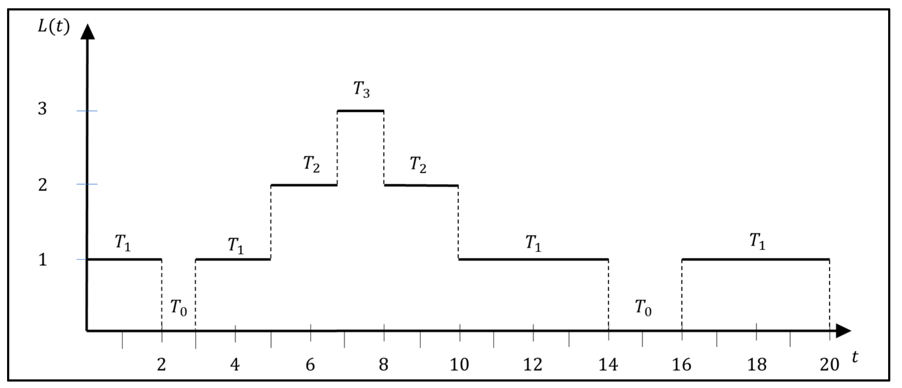
For a queueing system, one run of the simulation will result in a sample path that models the number of items in the queue during the time. The interarrival Z_i(t) and service time S_i(t), characterizing a generic i^th item entering the queue, are simulated by sampling the inverse of the distribution probability functions, Z⁻¹ and S⁻¹, characterizing the two processes. This allows one to construct a sample path of the system evolution that, as shown in Figure 5 [42], depicts for each discrete event time-point the number of items enqueued in the system. As it can be understood, the advantage of the Monte Carlo simulation is to overcome the limitation of the analytical “Little’s Law” which is valid only for the Poisson distribution and to generalize the modelling with the possibility to simulate the behaviour of a general queueing system.

For the reliability of a system, the MCS corresponds to performing an experiment for a certain mission time (${\mathrm{T}}_{\mathrm{M}}$) in which a large number of identical stochastic systems, each one behaving differently, runs virtually instead of performing real physical tests.

The simulation algorithm monitors whether a system fails before the completion of the mission and, in that case, records the time of the failure. This procedure corresponds to the observation of several realizations of the system process. Based on the amount of observations fallen into each range, simulation results are examined [41].

In a reliability problem, on the one hand, a set of possible states can be considered for a component (e.g., functioning, degraded and failed, as shown in Figure 6a), and based on its failure distribution, random numbers are generated for the duration that the component remains in each state; on the other hand, an infinite set of other states can be modelled considering how the failure rate h(t) changes over time, depending on the age of the component and on the boundary conditions in which it operates (Figure 6b).

Both these approaches overcome the hypothesis HP4 of dyadic states. With regard to the first, the sojourn time into a state (duration) is computed by the inverse distribution function F⁻¹ that characterizes the jump towards another state. To obtain the unreliability for a given time (t), the number of runs that have jumped into a failure state before the mission time can be divided by the total number of runs [43]. Figure 6a shows an example of the sample path generated by 6 runs of a simulation where the transitions among the three different states of the components occur at different times. For the example of Figure 6a, the component has reached the failed state in four out of the total six runs before “t”—therefore, the unreliability of the system, F(t) = 4/6.

With regard to the second, with reference to Figure 6b, modelling the failure rate evolution enables one to calculate the instantaneous reliability R(T) as the probability that the component survives over the next times step ΔT. If the jump from one time step to another can be written with a mathematical functional Г(F, t, ·), which is a combination of dynamic failure rates and deterministic (mechanical) system equations (with this latter taking into account the dynamic change of the component’s failure behaviour and the working conditions), it is possible to build a hybrid distribution function that overcomes the limitation of the hypotheses HP3, HP4 and HP5. This type of modelling reconfigures a reliability problem into a Dynamic Reliability problem where Г is a mathematical functional that depends on the stochastic distribution function of the failure rate F, the time variable t and (·) which represents all the other physical parameters included in the mechanical relationship. Moreover, for this type of problem, the numerical integration of the functional is carried on through adopting a time-step integration Δt_sim.

For the proposed case study, the time-step integration, Δt_sim, has been set to 1 h and the dynamic failure rate functional that depends on the environmental temperature can be written as follows:

$$\Delta {Г}_i=\frac{\beta }{{\alpha }_i}\left[{\left(\frac{t}{a_i}\right)}^{\beta -1}-{\left(\frac{t-\Delta t_{sim}}{{\alpha }_i}\right)}^{\beta -1}\right]$$

(16)

$${\alpha }_i=\{\begin{array}{c}{\alpha }_i={\alpha }_0\frac{T_0}{T_i} , if T_i>T_0\\ \\ {\alpha }_0 , otherwise\end{array}$$

(17)

$$T_i=Tm+A_T\sin \left(\frac{2\pi }{T}i\right)$$

(18)

The numerical integration of the functional $Г$ can be computed using the following formula:

$${Г}_{i+1}={Г}_i+\Delta {Г}_i$$

(19)

In order to overcome the hypothesis HP6, the restoration of a component can be modelled by sampling the generic repair distribution which will give the time-point at which the repair transition occurs and bring the component back to the functioning state (i.e., as good as new with a corrective maintenance policy). Therefore, in the repairable queue system, whenever the manufacturing station goes into the failed state, it is possible to assume that during the unavailable state, the queueing system cannot continue its processing (and thus decreases the number of items in the queue), but, eventually, it can be subject only to the arrival of new items. Only when the manufacturing station gets restored, the provision of service will start again. By assuming a general probability distribution of repair, it is possible to write the general discrete equation of the equipment unavailability that can be expressed as the ratio of the total accidental shutdown time over the total task time [31]:

$$U_{i+1}=\frac{\mathbb{E}\left({\tau }_u^{min}\right) \mathbb{E}({{\displaystyle \sum }}_0^{i+1}{Г}_{i+1})+\mathbb{E}\left({\tau }_p^{min}\right)}{i*\mathsf{\Delta }\mathrm{T}+\mathbb{E}\left({\tau }_p^{min}\right)}$$

(20)

where $\mathbb{E}\left({\tau }_u^{min}\right)$ is the expected value o on the jobs scheduling for the minimal repair duration, $\mathbb{E}\left({\tau }_p^{min}\right)$ is the expected value of the planned maintenance duration, $\mathbb{E}({\displaystyle \sum }_0^{i+1}{Г}_{i+1})$ is the the expected number of failures in the (i + 1)th timestep.

4.2. Simulation Execution of the Hybrid Monte Carlo Simulation Algorithm

This section describes the results of single iteration of the simulation process for the use case described in Section 4.1.

As explained in the previous section, the Discrete Event Table is initialized in Block.2 at the beginning of each iteration. For instance,

Table 3. Discrete Events Table of the generic ith run of the simulation of the items.

Job	Tmi (h)	tsm (h)	Measuring Unit
1	0	94	h
2	10	89	h
3	46	87	h
…	…	…	h
N	…	…	h

shows the main data-points event times of the ith jobs of a generic iteration, which are sampled using the inverse functions of Equations (11) and (12).

From Block.4, the continuous simulation starts, and

Table 4. Time-Driven Table of the generic iteration (run) of the simulation process.

SimTime	T(t) [°C]	α(T) [h]	ΔГ	Г	Random Number	Failure Test	Job Complete
0	20.0	100.0	-	0.000	0.3834	False	False
1	21.3	93.9	1.09 × 10−5	1.086 × 10−5	0.3831	False	False
2	22.5	88.9	2.14 × 10−5	3.222 × 10−5	0.9560	False	False
3	23.5	85.0	3.42 × 10−5	6.644 × 10−5	0.1671	False	False
…	…	…	…	…	…	…	False
80	24.3	82.2	9.13 × 10−5	2.52 × 10−2	0.0126	True	False
87	…	…	…	…	…	False	False
…	…	…	…	…	…	…	False
101	…	…	…	…	…	…	True

shows the evolution of the system that, among other things, depends on the physical mechanical equations of the system. The instantaneous dynamic failure rates are updated at any ΔT.

Let’s explain the meaning of each column for a better understanding of the paper.

• The column SimTime represents the time of simulation that increases according to the integration time step (Δtsim).
• The column ΔГ is the instantaneous failure rate of the machine tool, computed using Equation (16).
• The column α(T) is the expected mean life of the machine tool, computed using Equation (17).
• The column T(t) is the working temperature, computed using Equation (18).
• The column Г is the integral of the instantaneous failure rate functional.
• The column rand_num samples a uniform real random number in [0,1] to perform the failure test.

Therefore, in the failure test column is indicated the result performed in Block.9 to verify whether the machine tool of the service station becomes broken (Failure_Test = True) at that time point:

$$\mathrm{Failure} \mathrm{Test} =\{\begin{array}{c}\mathrm{False},{ \mathrm{if} \mathrm{e}}^{-Г}<\mathrm{rand}\_\mathrm{num} \\ \mathrm{True},{ \mathrm{if} \mathrm{e}}^{-Г}\ge \mathrm{rand}\_\mathrm{num}\end{array}$$

(21)

As shown in Table 3, it is possible to see that the Job 1 would require 94 hours to complete (see the t_sm column). From the evolution of the Time-Driven Table (Table 4), it is possible to notice that at time 80 h the machine tool becomes broken (see column “Failure Test” → True), and it resumes after 7 h. Therefore, the next row of the Time-Driven Table has the value SimTime = 87 h. In the end, the Job 1 completes at time SimTime = 101 hours (see column “Job Complete” True) so that the algorithm executes in Block.4 the next job. During that interval, the machine has gone under repair, Block.10; the simulation parameters are updated (Block.6), and the next time of failure for the service station is computed (Block.7 to Block.9).

Otherwise, if the service station is functioning, the simulation process keeps verifying when the i^th job has completed in Block.11. If it is not completed, the parameters are updated in the Block.6; otherwise, in Block.12, the simulation engine checks whether the jobs scheduled in Table 3 are completed. If there are other jobs to process, the simulation starts back from the Block.4; otherwise, the run of the simulation is complete.

4.3. Design of Experiment and Simulation Results

The case study has been analysed according to the design experiment of

Table 5. Design of experiments.

Scenario			0	1	2	3
Parameter Description	Symbol	Measuring Unit
pdf of interarrival time	$\mathsf{{\rm I}}$	-	neg exp	norm
mean interarrival time	tim	h	10	10	10	10
std. deviation of interarrival time	σti	h	10	2	2	2
pdf of service time	$\mathsf{{\rm Z}}$	-	neg exp	norm
mean service time	tsm	h	5	5	5	5
std. deviation of service time	σts	h	5	1	1	1
pdf of failure time	$\mathsf{\Lambda }$		#N/A		Weibull
service station expected life time	a0	h	-		100	100
shape factor	β		-		3	3
pdf of repair time	$\mathsf{\Phi }$		#N/A		Uniform
maintenance strategy			#N/A		Corrective
max restoration period	TTRmax	h	-		8	8
min restoration period	TTRmin	h	-		1	1

. The simulation scenarios 0 and 1 model a queueing system without failures, assuming interarrival and service times according to a negative exponential and a normal distribution; they are needed in order to validate the coded MCS and compare the results with closed analytical equations.

In scenarios 2 and 3, on the other hand, the restoration of the system and the evolution of the failure rate due to aging (scenario 2) and due to aging, wear and variations of the operating conditions (scenario 3) are modelled.

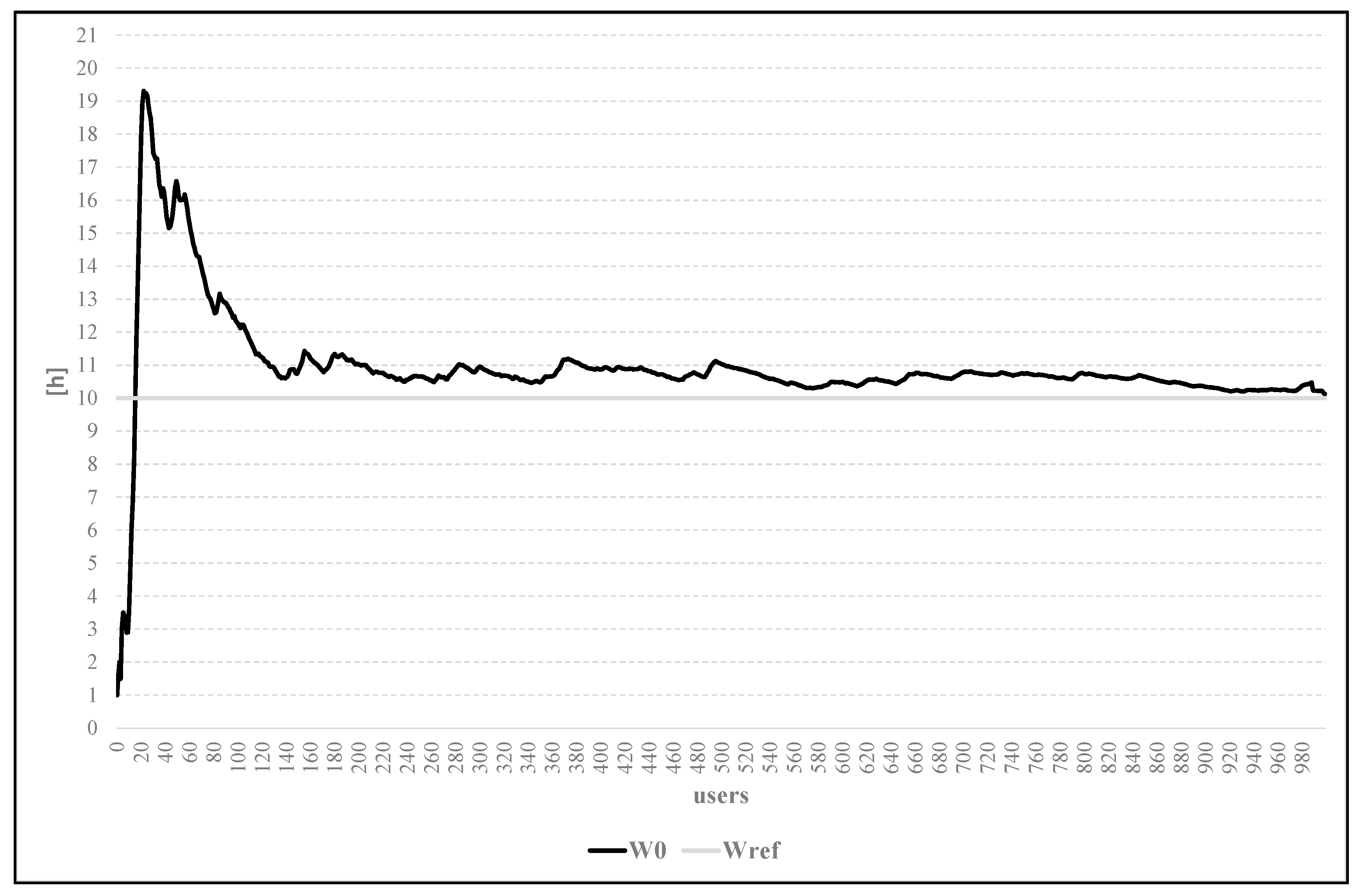
Figure 7 shows the comparison between the simulative process and the analytic benchmark of scenarios 0. With 10³ runs of the simulation, it is possible to observe that the two models converge. In particular, the simulated mean awaiting in queue time is W₀ = 10.12 h, and the analytic mean awaiting queue time W_ref = 10.0 h (mean error $\Delta e=\frac{W_0-W_{ref}}{W_{ref}}=1.12 \%$).

The simulation results of scenario 1 show that the mean waiting time is 5 h. With regard to this scenario, inferential statistics enables one to define an upper bound for mean waiting time in queue according to the following equation [44]:

$$E(W_q)\le \frac{{\sigma }_{ti}^2+{\sigma }_{ts}^2}{t{i}_m\left(1-\rho \right)}=7 \mathrm{h}$$

(22)

where p = ts_m/ti_m is the level of service utilization; σ_ti and σ_ts are the standard deviations, respectively, of interarrival and service time; ti_m is the mean interarrival time. Both the previous results confirm the goodness of the MCS coded.

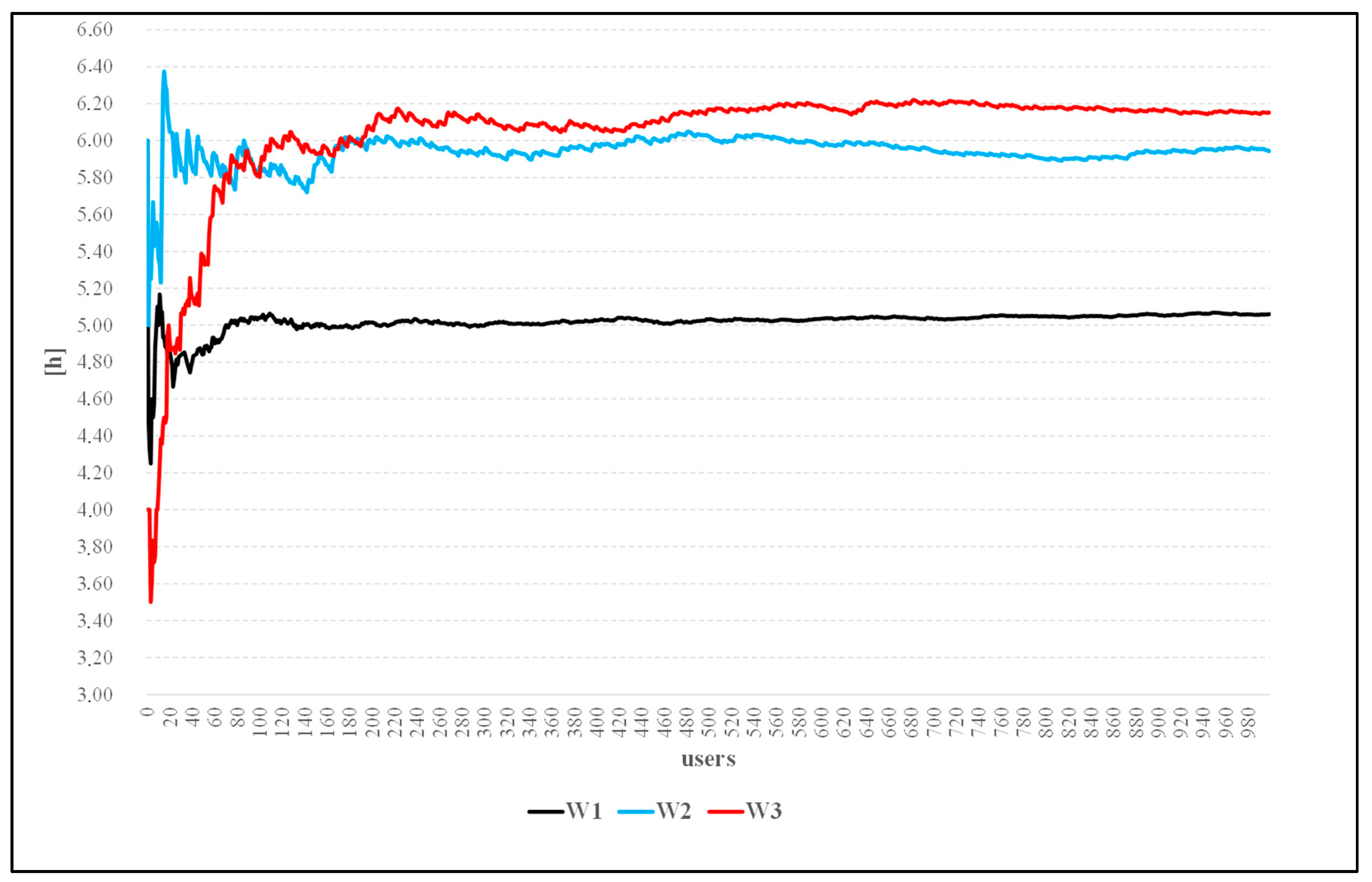
Figure 8 shows the Monte Carlo simulation process of the progressive mean waiting time of Scenarios 1–3. The reported trends allow a person to conclude that the average waiting time in queue increases with the increased complexity of the operative scenario.

In fact, Scenario 1 which characterizes a system that cannot fail (max reliability of the system) shows the shortest mean waiting time in the queue. In Scenarios 2 and 3, the mean waiting time increases due to the increasing unavailability of the service station caused by the modelling of the failure rate. In particular for Scenario 2, this result is mainly given by the aging of the service station; whereas in Scenario 3, this effect is more emphasized by the contribution of the operating temperature.

The results given by the simulation shows that the average waiting in queue time is, respectively, W1 = 5.0 h; W2 = 5.94 h; W3 = 6.12 h. These cannot be compared with an analytical benchmark because, as explained, the modelling and evaluation of such scenarios are not doable with analytical methods. Finally, only for the Scenarios 2 and 3, the model has been used to evaluate the system’s availability, the mean waiting time in queue and the mean number of jobs in queue for different level of service utilization r = [0.5; 0.6; 0.7; 0.8; 0.9; 0.95; 0.99]. As shown in

Table 6. Performances of the system (ts_mean = [5, 6, 7, 8, 9, 9.5, 9.9]; σ_ts = 0.2 ts_mean).

r	W2	W3	A2	A3	L2	L3
	[h]	[h]
0.5	5.9	6.03	86.9%	84.8%	0.57	0.60
0.6	7.4	7.68	86.9%	84.8%	0.71	0.79
0.7	9.2	9.51	86.9%	84.8%	0.94	0.96
0.8	11.8	13.54	86.9%	84.8%	1.17	1.36
0.9	96.0	188.35	86.9%	84.8%	9.37	18.05
0.95	451.9	472.04	86.9%	84.8%	41.38	43.21
0.99	708.0	811.60	86.9%	84.8%	62.77	70.85

, this subset of scenarios confirms that the performances of the queueing system decrease when operational conditions and aging are considered, and this is more emphasized in Scenario 3 (W_i: Mean waiting time in the queue; A_i: Availability of the machine tool; L_i: Mean items in the queueing system).

5. Conclusions and Remarks

The importance of a more realistic modelling and evaluation of the manufacturing and production processes is becoming a key component in the success of modern enterprises which are called upon to be agile and reactive to the market demand. The revolution brought with Industry 4.0 is helping to automate and digitalize such processes allowing us to collect the relevant information to identify bottlenecks and reveal opportunities to increase the throughput of the system processes.

In this paper, the performance evaluation of a production system has been addressed by the implementation of a simulation model of a repairable G/G/1 queueing system with a corrective maintenance policy. The model has been coded adopting a hybrid dynamic dependability approach able to link the aging and the wearing of the queuing system to the change of the working conditions, using the mechanical equations of the wearing physical process. The rationale behind the proposed approach is that the real-time information produced by the smart factories are now significant and help to extract, and thus model, with more precision the characteristics of the general stochastic processes and to find out the relationship between the working conditions and the wearing of the system. The simulation proposed represents a powerful tool in comparison with the analytical theoretical queueing models of the referred literature because it has been implemented in order to combine the physics of the system with the stochastic processes of the queuing theory and reliability. This has allowed us to consider in the model not only the randomness of the queue and of the machine reliability but also how the operational conditions affect these two processes. Moreover, a simple—yet valuable—corrective maintenance is analysed, but the simulation tool could be eventually improved to model, also, a preventive maintenance policy.

As expected, the results of the analysis performed into the G/G/1 with corrective maintenance show that the throughput of the system (mean waiting in queue) improves with the increasing of the system reliability; but, on the other hand, it demonstrates the importance of such advanced modelling tools that are able to take into account the influences caused by the working conditions on real production scenarios. The Monte Carlo simulation model has been coded using the electronic spreadsheet that—by means of the industrial connectors plug-in (ODBC, Modbus, IoT, OPC, etc.)—can be easily integrated into the manufacturing process. This demonstrates, on the one hand, that it is possible to code a complex simulation scenario (Event Driven with Continuous input data) in this software environment and that it can be used to analyse the system performance or to evaluate how to improve the weak elements of a production process, even before any engineering refactoring. Under this viewpoint, in future works, the model can be improved in order to handle other types of maintenance policies and compare the performance and the costs with respect to the corrective maintenance policy.

From the management point of view, the paper demonstrates that it is possible to develop a simulation model that can allow one to estimate the performance of the production line with tools which are not too complex or expensive, having a good knowledge of the business processes and of mathematical reliability and queuing theory. The proposed model, moreover, offers the possibility to modify the probability distributions of the queueing and reliability processes which can be customized ad hoc, depending on the production line modelled. This allows a person not only to estimate the performance of the system as it is, but also to analyse what modifications can be brought to the production line in order to understand the effects and the possible improvements.

Of course, the proposed approach presents some limitation. For instance, the Electronic Spreadsheet is not general enough to model any production scenario which could require an ad hoc model of the system and tuning of the model. Therefore, further research should identify other tools and generalize the proposed modelling in order to improve the effectiveness of the Monte Carlo simulation hybrid approach discussed.