Research on Leakage Location of Pipeline Based on Module Maximum Denoising

Abstract

Leak detection and location of water supply pipelines is an important area of research, and it is especially important to find the leakage location in time and repair them. In view of the problem, that a large amount of noise is mixed in the detection signal when the pipeline leaks, it will inevitably affect the detection and positioning effect. In this paper, a denoising algorithm based on improved module maximum is proposed. Firstly, a discrete binary wavelet transform is carried out on the noisy signal, and the module maximum point corresponding to the wavelet transform coefficients, on each scale, is obtained. Secondly, different thresholds are used for the module maximum of different scale layers and the wavelet coefficients are reconstructed according to the retained module maximum and their extremums. Thirdly, the alternative projection algorithm is used to effectively suppress the false oscillations in the reconstructed signal, improve the quality of the reconstructed signal, and obtain the noise reduction signal. Finally, according to the theory of the negative pressure wave, the inflection point of the negative pressure wave is identified by the wavelet decomposition method, and the location of leakage point is determined. In order to verify the effectiveness of the proposed algorithm, a leakage simulation experiment system of water supply pipeline is built. The analysis of the results shows that, compared with the wavelet denoising method and the EMD-based method, the method proposed in this paper achieves a better denoising effect, obtains a smoother pressure signal, retains the signal waveform characteristics, and identifies the obvious inflexion point of the negative pressure wave. The minimum relative error of leakage point location is 0.9%, and the maximum relative error is 2.5%.

1. Introduction

Pipelines are one of the most affordable solutions for moving large amounts of oil, gas, chemicals, and water onshore, with the advantages of large volume, continuous operation, low cost, and freedom from climate impacts and other constraints [1]. As of 2014, the total length of pipeline used for global transportation is about 3.8 billion meters [2]. However, in recent years, due to the aging of pipelines, man-made damage and other reasons, pipeline explosions, ruptures, leakage, and other accidents occur frequently, which may bring problems to users and the environment. According to statistics, the average leakage of the water supply network is about 15.7% in China [3,4]. The leakage of the water supply network not only increases the cost of water supply facilities, but also increases the probability of secondary disasters. Therefore, reducing pipe network leakage and saving water resources is an important responsibility of today’s society.

At present, the commonly used methods for pipeline leakage detection include the flow balance method, infrared thermal imaging method, pressure gradient method, and negative pressure wave method.

The basic principle of the flow balance method is that when a leak occurs in the water supply pipeline, the water flow in the pipe will flow out quickly from the leakage point, and the flow downstream of the leakage point will be significantly smaller than that upstream, so by calculating the change in the flow of the pipeline section, it can be judged whether there is leakage. However, the method cannot locate the pipeline leakage point [5].

The second method is the infrared thermal imaging method. When the water supply pipeline is damaged, the water flow in the pipeline will spread to the soil around the leakage point. As the wet soil heat dissipation speed is faster, the heat contained in the soil around the pipeline leakage point will be significantly different from the heat contained in other soils. However, the infrared thermal imaging method requires relatively high theoretical knowledge by staff, who must master the infrared spectrum analysis technology skillfully, and the cost of the instruments required for detection is also very high. These shortcomings make it difficult for infrared spectrum thermal imaging to be popularized in China [6].

The basic principle of the pressure gradient method is that when the water supply pipeline is operating normally, the pressure in the pipeline usually changes linearly along the pipeline. But when the pipeline leaks and reaches a stable state again over time, the pressure signal at the leakage point of the pipeline will have an obvious change. By comparing the difference of the pressure gradient curve before and after leakage, the extent of pipeline leakage and the location of pipeline leakage point can be determined. This method is usually greatly affected by the accuracy of the instrument and the environment in which the measuring instrument is located.

The method of leak location based on the negative pressure wave (NPW) has become one of the research hotspots [7,8,9]. When the pipeline leaks, the pressure at the leakage point will drop rapidly, and this pressure drop named the NPW inflection point will propagate to both sides of the leakage point in the form of a negative pressure wave. The leakage can be detected by installing pressure sensors on both sides of the pipeline to obtain changes in the pressure signal in the pipe. The time difference between the two negative pressure wave signals can be used to determine the leakage location [10]. The method based on NPW signal has the advantages of low price, easy operation, long transmission distance, and high stability accuracy. So, the research in this paper will be based on the negative pressure wave theory.

The sensor will inevitably mix some noise in the process of NPW signal acquisition. The noise will reduce the Signal-to-noise ratio (SNR) of the detected signal, and even drown the useful signal in serious cases, which will lead to locating the leak extremely difficult. Therefore, it is very necessary to denoise the signals collected by the sensor to reduce or eliminate noise and extract useful signals.

Because wavelet transform has good time-frequency characteristics, different frequency components of signal can be decomposed by the wavelet transform, which has been widely used in signal denoising. The principle of wavelet threshold denoising is select the appropriate wavelet basis function and the number of decomposition layers to achieve adaptive signal decomposition, and then reconstruct the signal according to the threshold (hard threshold or soft threshold) function. The hard threshold function is superior to the soft threshold method in the sense of mean squared error, but the signal generates additional oscillations and jump points, and this discontinuity leads to the pseudo-Gibbs phenomenon in the reconstructed signal. The wavelet coefficient estimated by the soft threshold function has good overall continuity, and the estimated signal does not easily produce additional oscillations, but there is a large deviation between the estimated value and the actual value [11,12].

Variational mode decomposition (VMD) is an adaptive signal decomposition method proposed by Dragomiretskiy, in 2014 [13,14]. Compared with wavelet decomposition, VMD can effectively suppress the phenomenon of modal aliasing and over-decomposition, and while it does not rely on intrinsic basis functions, it can adaptively decompose the signal into multiple intrinsic mode functions (IMF), from high to low frequency, and can achieve signal noise reduction by screening effective component reconstruction. However, there are still some limitations to the use of VMD. Before VMD decomposition of the signal, the number of modes K and the quadratic penalty term α should be set in advance. In many cases, prior knowledge of the signal is unknown. If K and α are not chosen properly, too few or too many modes will be generated, resulting in signal component loss or more noise.

The module maximum method is a classical denoising algorithm, the module maximum amplitude of noise decreases rapidly with the increase of the scale, and the normal signal increases with the increase of the scale, so the noise can be removed from the normal signal. However, the signal after noise reduction has glitches and slight oscillations.

In order to realize effective denoising of the actual signal, the advantages of the above methods are combined, and an improved module maximum denoising algorithm is proposed in this paper. Firstly, a discrete binary wavelet transform is used to find out the module maximum, corresponding to the wavelet transform coefficient on scale J. Different threshold values are used to deal with the maxima of different scale modes, which can avoid the loss of signal components and the introduction of new noise. Finally, the NPW theory is used to locate the leakage point. Experimental results show that this method effectively improves the lack of adaptability of the traditional methods, and it can acquire a clear NPW inflection point. By using the same data, the proposed method can obtain the highest SNR. Thus, the noise suppression of our method is more effective.

The structure of this paper is as follows: In Section 1, the research background of this paper, and some commonly used pipeline leakage detection methods and negative pressure wave signal denoising methods are introduced. The method proposed in this paper is also briefly introduced. In Section 2, the noise reduction principle of the method based on improved module maximum is introduced in detail. Section 3 is the experimental environment and leak point layout, and the results and discussion. The practicability and advantages of our method are verified. Finally, the conclusion is given in Section 4.

2. Materials and Method

2.1. A Novel Denoising Method Based on Improved Module Maximum

2.1.1. Discrete Wavelet Transforms and Module Maximum

Discrete wavelet transform can be realized using the Mallat algorithm. It carries out repeated low-pass and high-pass filtering for discrete signals through wavelet filter, and a low-frequency signal and a high-frequency signal can be obtained each time. Then low-pass and high-pass filtering are performed on the low-frequency signal again, and the low-frequency signals on the larger decomposition layer can be obtained. Therefore, the result of the discrete wavelet transform of a discrete signal should include the high frequency component at each level and the low frequency component at the maximum level. The advantage of this processing is that any detail of the signal can be noticed.

In this paper, the discrete wavelet transform is applied to the noisy signal, and the module maximum value corresponding to the wavelet transform coefficients on each scale is obtained. The specific process is as follows:

Let the parent wave function be $\Psi (t)$, the scaling and translation factors are a and b, and the wavelet basis function is:

$${\Psi }_{\mathrm{a},b}(t)=\frac{1}{\sqrt{a}}\Psi \left(\frac{t-b}{a}\right)$$

(1)

where, a and b are real numbers.

There is a function $f(t)\in L^2(R)$, whose wavelet transform can be defined as $W_{a,b}(f)$:

$$W_{a,b}(f)=<f(t),{\Psi }_{a,b}(t)>f(t)=\frac{1}{\sqrt{a}}{\int }_{-\infty }^{\infty }f(t){\Psi }_{a,b}(t)dt$$

(2)

Then the wavelet transform $W_{a,b}(f)$ is the decomposition of the function $f(t)\in L^2(R)$ on the corresponding function family ${\Psi }_{a,b}(t)$, and the premise of decomposition is that the parent wave function $\Psi (t)$ satisfies the following allowable conditions:

$$C_{\Psi }=\underset{k\to \infty }{\lim }{\int }_0^k\frac{|\Psi (\widehat{w})|}{w}dw$$

(3)

In the formula, $\Psi (\widehat{w})$ is the Fourier transform of $\Psi (t)$.

In order to improve computational efficiency, wavelet transform can adopt convolution form:

$$W_{s}f(t)=f(t)\ast {\Psi }_s(t)=\frac{1}{s}{\int }_{-\infty }^{\infty }f(x)\Psi \left(\frac{t-x}{s}\right)dx$$

(4)

where ${\Psi }_s(t)=\frac{1}{s}\Psi \left(\frac{t}{s}\right)$. s is the scale parameter. In practical application, the scale parameter of the wavelet transform does not need to be evaluated continuously. The usual processing method is the binary separation of the scale parameters. That is $s=2^j$, $j$ is an integer, and the wavelet transformation of the noisy signal at the scale $2^j$ is:

$$W_{2^j}f(t)=f(t)\ast {\Psi }_{2^j}(t)=\frac{1}{2^j}{\int }_{-\infty }^{\infty }f(x)\Psi \left(\frac{t-x}{2^j}\right)dx$$

(5)

The results of Formula (5) can be used to describe the local information of the j-th octave of the noisy signal.

Based on the binary discrete wavelet transform, the process of solving module maximum in this paper is as follows:

For any point x in a neighborhood of x₀, there is a condition $|W_f(s,x)|\le |W_f(s,x_0)|$ for any point in the neighborhood of x₀ [15]. Let $W_f(s,x)$ be the convolution wavelet transform of f(x). Under the scale s₀, point (s₀, x₀) is called the local extreme point. If $\frac{\partial W_f(s_0,x_0)}{\partial x}$ is 0 at $x_0$, then (s₀, x₀) is considered to be the module maximum point of the wavelet transform [16].

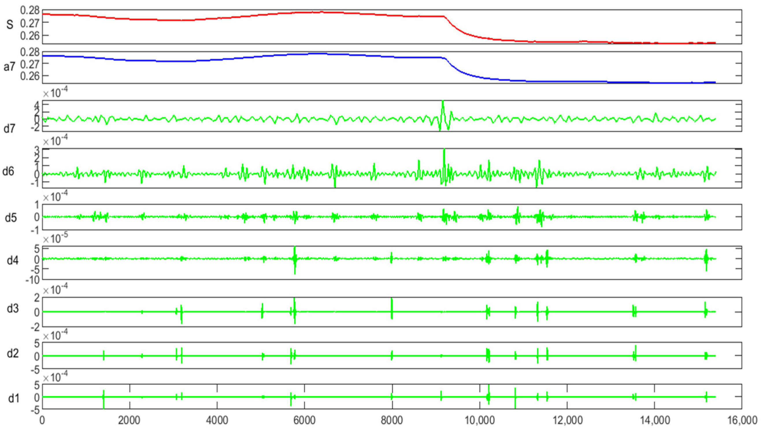
2.1.2. Singularity Analysis and Threshold Processing of Signal and Noise

When the noisy signal $x$ is in the interval $[a,b]$, the wavelet transform $f(x)$ satisfies:

$$\left|W_f(s,x)\right|\le k{s}^{\alpha }$$

(6)

where, k is constant, and $\alpha$ is the Lipschitz index. The Lipschitz index will be used to describe singularity. The larger the Lipschitz index, the higher the smoothness of the signal points, and vice versa. If a bounded function is continuous and differentiable at a point, or if it has a derivative at that point but the derivative is discontinuous, then the Lipschitz index is 1. By taking logarithm of both sides of the inequality (6), Lipschitz index of the signal $f(x)$ has the following relation with the module maximum of the wavelet transform: if the singularity of the real signal x is greater than zero, the maximum modulus of the wavelet transform increases with the scale. If the singularity of the signal is negative, the opposite is true. In general, the Lipschitz index of the noise function is less than zero. The noise singularity is often large in the one-dimensional signal, and the Lipschitz index is less than −0.5.

The wavelet technique is used to decompose the original signal. With the increase of scale J, the average amplitude and density of the module maximum point with noise component will decrease [17].

Signal decomposition generally starts from the maximum decomposition scale J, the threshold $Thr=C*M/J$ is set on the scale J, and the module maximum point that should be retained on the maximum scale is determined by adjusting variables. Where C is the threshold parameter, according to reference [18], its value can be taken as 0.8. M is the maximum value of all module maximum in scale J [18], and it is the maximum value obtained by comparing the absolute value of the modular maximum sequence with the threshold value. Points with values less than the threshold value become zero, and points with values greater than or equal to the threshold value remain unchanged, that is, the module maximum corresponding to the position of the mutation point is retained. Although the signal characteristics can be preserved by this method, the denoised signal has burrs and slight oscillations at the singularities. The main reason is that the wavelet transform value is discontinuous at the threshold after extracting the module maximum corresponding to the position of the mutation point. In order to overcome this shortcoming, soft threshold processing can be performed on the modular maximum sequence, and the soft threshold function is:

$${\tilde{w}}_{jk}=\left\{\begin{array}{cc}{w}_{jk}-\lambda & w_{jk}⩾\lambda \\ 0& \left|w_{jk}\right|<\lambda \\ w_{jk}+\lambda & w_{jk}⩽-\lambda \end{array}\right.$$

(7)

In the formula, $w_{jk}$ is the wavelet coefficient and $\lambda$ is the threshold value. The wavelet coefficient is greatly affected by noise at small scales, resulting in many pseudo-extreme points, and often the location of the mutation point cannot be located by only one scale. At large scales, the signal is processed with a certain smooth soft threshold, and the extreme value points are relatively stable. When determining the singularity of the signal by the wavelet transform module maximum method, it is necessary to combine multi-scale comprehensive observation.

2.1.3. Signal Decomposition and Reconstruction Principle

The Mallat algorithm convolves the vector (low frequency) to obtain low frequency information. The vectors are then also convolved to obtain high frequency information. The frequency of the signal changes with time, and this change can be divided into two parts: slow change and fast change. The slow change part corresponds to the low-frequency part of the signal, representing the main outline of the signal, while the fast change part corresponds to the high-frequency part of the signal, indicating the details of the signal.

Let $\varphi (t)$ and $\phi (t)$ be the scale function and wavelet function of the function $f(t)$ at $2^{j-1}$—resolution approximation, respectively, then its discrete approximation part $A_{j}f(t)$ and detail part $D_{j}f(t)$ can be expressed as:

$$A_{j}f(t)={\displaystyle \sum }_{k=-\infty }^{\infty }{C}_{j,k}{\varphi }_{j,k}(t)$$

(8)

$$D_{j}f(t)={\displaystyle \sum }_{m=-\infty }^{\infty }{D}_{j,m}{\psi }_{j,m}(t)$$

(9)

According to the decomposition idea of Mallat’s algorithm, $A_{j}f(t)$ is decomposed into rough part $A_{j+1}f(t)$ and the detailed part $D_{j+1}f(t)$:

$$A_{j}f(t)=A_{j+1}f(t)+D_{j+1}f(t)$$

(10)

where $A_{j+1}f(t)={\displaystyle \sum _{m=-\infty }^{\infty }{C}_{j+1,m}{\varphi }_{j+1,m}(t)}$; $D_{j+1}f(t)={\displaystyle \sum _{m=-\infty }^{\infty }{D}_{j+1,m}{\psi }_{j+1,m}(t)}$.

$${\displaystyle \sum }_{m=-\infty }^{\infty }{C}_{j+1,m}{\varphi }_{j+1,m}(t)+{\displaystyle \sum }_{m=-\infty }^{\infty }{D}_{j+1,m}{\psi }_{j+1,m}(t)={\displaystyle \sum }_{k=-\infty }^{\infty }{C}_{j,k}{\varphi }_{j,k}(t)$$

(11)

where, $C_{j+1,m}$ and $D_{j+1,m}$ are the expansion coefficients on the scale, and the former is the scale coefficient, and the latter is the wavelet coefficient.

From a two-scale equation: $\left\{\begin{array}{l}\varphi =\sqrt{2}{\displaystyle \sum _{k=-\infty }^{\infty }h}(t)\varphi (2t-k)\hfill \\ \Psi =\sqrt{2}{\displaystyle \sum _{k=-\infty }^{\infty }g}(k)\varphi (2t-k)\hfill \end{array}\right.$ and orthogonality:

$$C_{j+1,m}={\displaystyle \sum }_{k=-\infty }^{\infty }{h}^{\ast }(k-2m)C_{j,k}$$

(12)

$$D_{j+1,m}={\displaystyle \sum }_{k=-\infty }^{\infty }{g}^{\ast }(k-2m)C_{j,k}$$

(13)

$$C_{j,k}={\displaystyle \sum }_{k=-\infty }^{\infty }h(k-2m)D_{j+1,m}+{\displaystyle \sum }_{k=-\infty }^{\infty }g(k-2m)D_{j+1,m}$$

(14)

So, we can perform fast wavelet decomposition and reconstruction of the signal according to the above formula.

In summary, the denoising process of the algorithm proposed in this paper is as follows:

Step 1: Perform a wavelet transformation on the noisy signal, and find the module maximum value of the transformation coefficient on each scale, and the maximum value of J is generally 4 to 6.

Step 2: Starting from the largest scale, a threshold is determined according to the scale. The module maximum point greater than the threshold is retained on this maximum scale, and the modulo extreme point less than the threshold is removed to obtain a new module maximum sequence on the maximum scale.

Step 3: On scale $J-1$, set the threshold $Thr=C*M^2/\log (J+1)$ to determine whether its module maximum point is greater than the threshold on its scale, and leave the maximum point greater than and in the search region corresponding to scale $J$ otherwise zeroed. Soft threshold function processing can also be considered: soft threshold processing is performed on the module maximum sequence to obtain a new set of module maximum points on the maximum scale.

Step 4: Repeat step 2 with $J=J-1$ until $J=2$.

Step 5: On the extreme point position saved at $J=2$, find the corresponding extreme point at $J=1$, and remove it.

Step 6: Use the modulus extremum points retained on multiple scales and reconstruct them by the interleaved projection method.

Step 7: The denoising signal will be used for leak detection and location of water supply pipelines.

2.2. Leakage Point Location Method

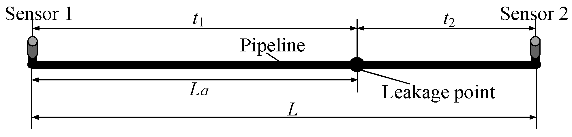
2.2.1. Negative Pressure Wave Theory

The negative pressure wave (NPW) method is a very effective and mature technology in pipeline leakage location applications. The delay of the signal is calculated by collecting leakage signals, at the head and end of the pipe, using sensors to estimate where the leak occurred. The positioning schematic is shown in Figure 1.

Two pressure sensors are installed on the water supply pipe. The leak point is located between the two sensors. If a leak occurs, the fluid pressure at that leak point drops and this negative pressure wave change is transmitted up (towards sensor 1), and down (towards sensor 2) along the pipe. Based on the velocity of the negative pressure wave, the time difference between the two pressure sensors and the distance between the sensors, the location of the leak can be determined.

It can be assumed that the distance between the two sensors is $L$ and the propagation speed of the negative pressure wave is $v$. The position of sensor 1 is set as the reference starting point. Assuming that the leakage point is located at position $X$, and the arrival time of the sensors at both ends of the pipe for NPW are $t_1$ and $t_2$, respectively, the time difference can be calculated according to the point corresponding to the inflection point of the negative pressure wave, so as to locate the leakage point. The calculation formula is as follows:

$${\rm T}t=\frac{n_1-n_2}{f}$$

(15)

In the formula, $n_1$ and $n_2$ are the locations of the inflection points where the NPW is detected, and $f$ is the sampling rate of the acquired signal.

The pipeline leak location formula is:

$$L_A=\frac{1}{2}(L+v{\rm T}t)$$

(16)

Therefore, the wave velocity $v$ of NPW and the time difference ${\rm T}t$, between the NPW reaching the upstream and downstream, are two key factors affecting the accuracy of positioning.

2.2.2. Calculation of NPW Velocity

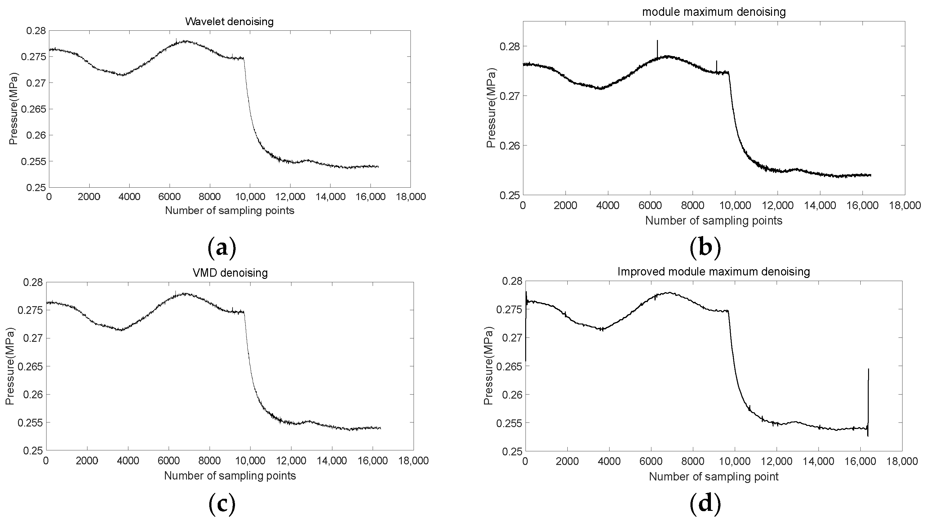
The propagation speed of the NPW is related to the characteristics of fluid and the properties of pipelines. As such, the calculation formula of NPW velocity is as follows:

$$v=\sqrt{\frac{K/\rho }{1+\frac{KD}{Ee}{C}_1}}$$

(17)

In the formula, $K$ is the bulk elastic modulus of water, Pa; $\rho$ is the density of water, Kg/m³; $E$ is the elastic modulus of the pipe material, Pa; $e$ is the thickness of the pipe, m; $D$ is the inner diameter of the pipeline, m; and $C_1$ is the coefficient of correction. When the pipe characteristics are known, the NPW velocity can be calculated.

3. Results

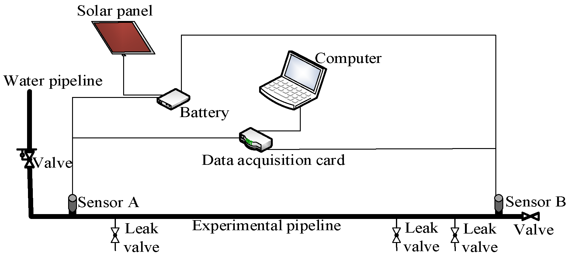
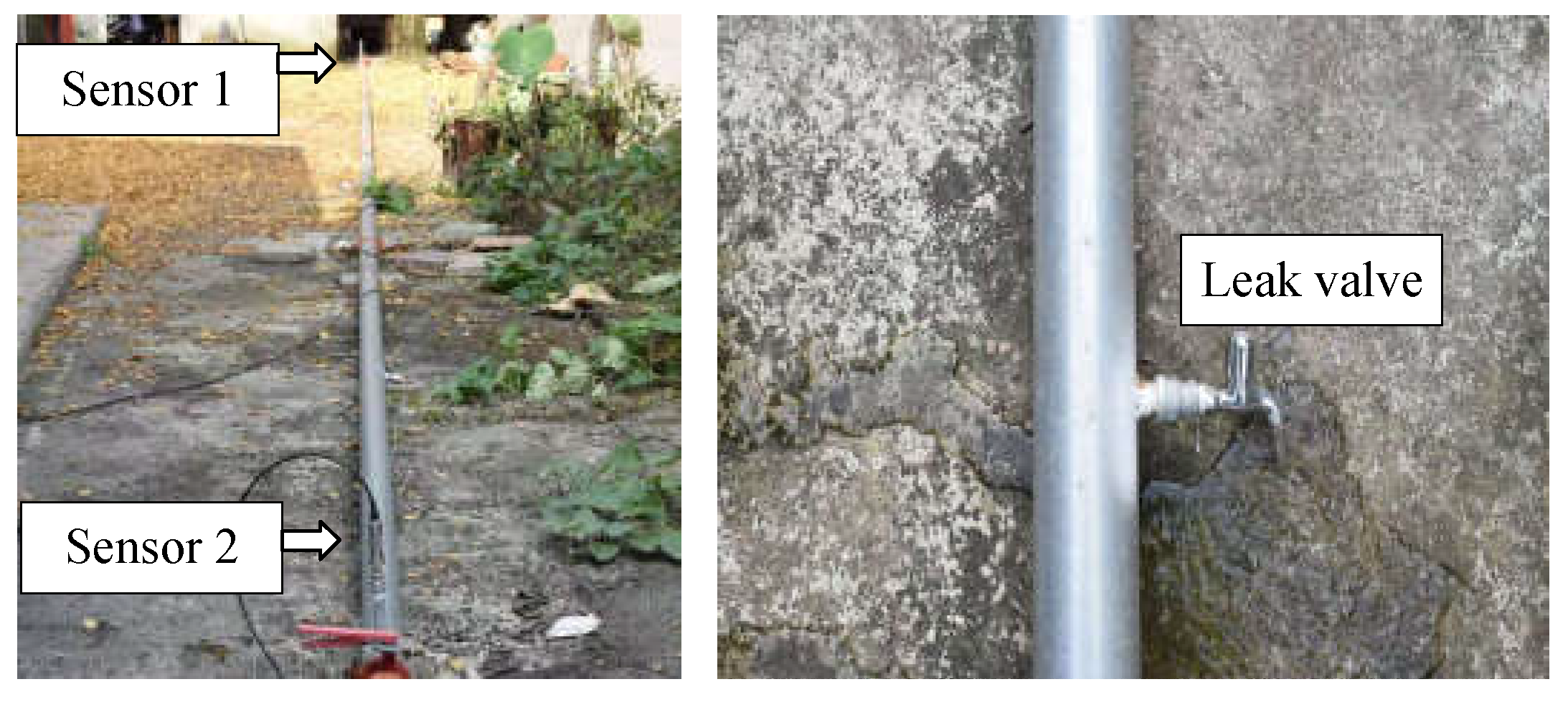
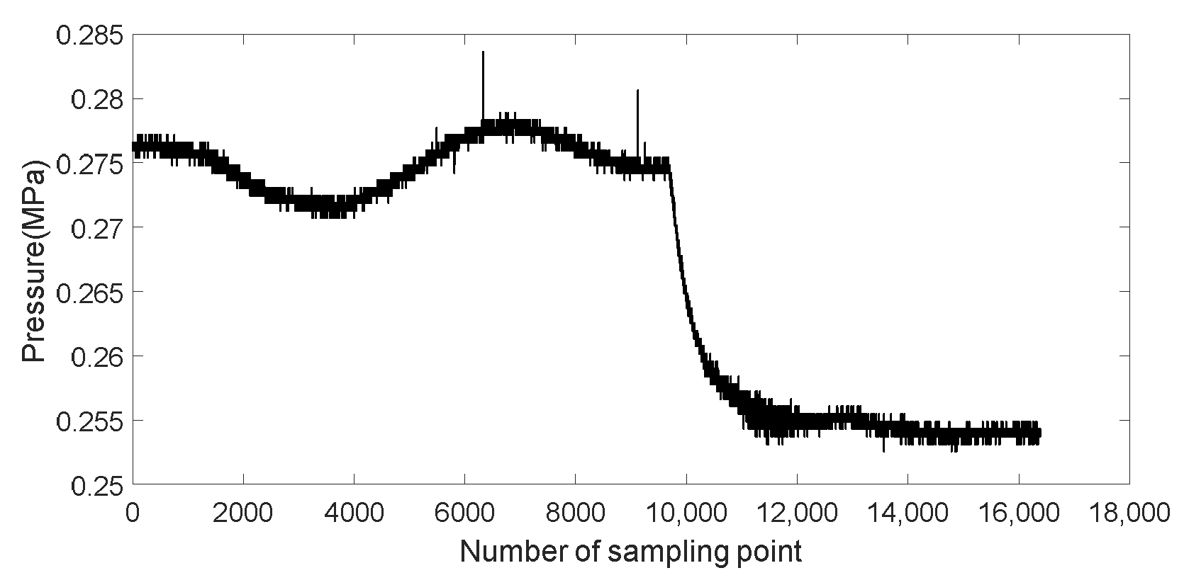
3.1. Verification by Experiment

The pipeline leakage experiment system as shown in Figure 2 is built. The leakage simulation system is shown in Figure 3, and the acquisition equipment is shown in Figure 4. The pipe is supplied by connection to an external water supply pipe. The pipe material is Q235B steel, the inner diameter is 80 mm, and the pipe wall thickness is 3 mm. To simulate a leak, the faucet can be opened quickly. The pressure signal is collected by a high-frequency dynamic pressure sensor with a range of 0~0.6 MPa. The battery is charged via a solar panel to power the sensor. The data acquisition card is used to collect the signal of the sensor and transmit it to the computer. The signal sampling frequency is 2 kHz, and the pressure in the pipeline fluctuates between 0.16~0.24 MPa. When the pipeline pressure drops by more than 0.1 MPa in a short time, a leak is considered to have occurred. The 3 valves used to simulate leakage in the pipeline are fully opened, half-opened, and then closed in turn, with signal data received from the two pressure sensors.

Considering the influence of the decomposition level on the algorithm, this paper first analyzes the influence of this key parameter on the signal-to-noise ratio, based on the experimental data, and the results are shown in Figure 5.

From Figure 5, it can be seen that for the experimental system in this paper, the best denoising effect can be achieved when the number of the decomposition layer is 5.

According to the pipeline parameters shown in

Table 1. The pipeline parameters.

Pipe inner diameter (m)	0.08
The density of water (kg/m3)	998.203
Pipe wall thickness (m)	0.003
The volumetric elastic modulus of water (Pa)	2.1 × 108
The elastic modulus of the pipe (Pa)	2.1 × 1011
Sampling frequency (kHz)	2
The pressure of the pipe (MPa)	0.16~0.24

, the negative pressure wave velocity is calibrated as 462.5 m/s.

Figure 6 shows the change of pressure signal when simulated leak point 2 is fully opened. As can be seen from Figure 6, the original signal contains a large amount of noise.

In order to verify the effectiveness of the proposed method, we use wavelet denoising method, modular maximum method, VMD denoising method and the proposed method to denoise the signal respectively. The result is shown in Figure 7.

Figure 7a shows wavelet denoising, Figure 7b shows module maximum denoising, Figure 7c shows VMD denoising, and Figure 7d shows improved module maximum denoising. It can be seen from the denoising results of each method in Figure 7 that the improved module maximum denoising proposed in this paper achieves the best denoising effect while preserving the original signal characteristics as much as possible. It causes a spike at the stop point of the signal due to local extreme points, because there is no subsequent signal for scale iteration, and scale preservation cannot be performed. According to the denoising effect shown in Figure 7, it can be seen that the improved module maximum denoising can best retain the original signal, suppress the noise signal. It can more truly reflect the detailed changes of the original signal, especially for the detection of pressure abrupt points caused by NPW. Our method can retain the characteristics of the peak signal at the inflection point in the one-dimensional sequence with almost a straight drop of press, which provides a basis for the accuracy of extracting the singularity (inflection point), by wavelet decomposition. The SNR of the four methods is as follows: VMD is 40.87, wavelet threshold is 43.90, module maximum is 44.01, and improved module maximum is 50.97. It also further illustrates that the denoising effect of the proposed method in this paper is better than the other three methods.

In order to verify the universality of the proposed method, the leakage simulation experiment is carried out on the other two leakage points, under three working conditions with different open valve areas. The above four denoising methods are adopted to calculate the average SNR after denoising. The results are shown in

Table 2. Average SNR calculation results.

Denoising Algorithm	SNR1	SNR2	SNR3
VMD	1.77	18.33	35.45
Wavelet	0.42	19.11	38.16
module maximum	1.43	30.24	48.21
Improved module maximum	1.96	35.55	51.80

:

Where SNR1 is the signal to noise ratio after signal denoising by several algorithms, under the condition that the water valve is opened to 5° (corresponding leakage area is 2 mm²), SNR2 is the signal to noise ratio after signal denoising by several algorithms under the condition that the water valve is opened to 45° (corresponding leakage area is 15 mm²), SNR3 is the signal to noise ratio after signal denoising by several algorithms under the condition that the water valve is opened to 90° (corresponding leakage area is 25 mm²). From the above table of results, it can be seen that the denoising effect of the proposed method in this paper is the best.

3.2. Leakage Location

Wavelets have the role of a “mathematical microscope”, which can make the characteristics of abnormal information of the pressure abrupt point, caused by pipeline leakage, more clear. According to the experiment, we found that the number of wavelet decomposition layer is 7, as shown Figure 8. S is the NPW signal after denoising, and a7 is the low-frequency signal part after decomposition. The high frequency part d is the description of the signal change. The more the signal changes, the greater the value of d, and vice versa. At that position, it can be seen from Figure 8 that when the number of decomposition layers is 7, the pressure drop inflection point of NPW can be well captured. In the NPW signal, the low frequency part describes the details of the signal, and the high frequency part describes the change of the signal. The more drastic the signal change, the greater the value of the decomposition layer, and vice versa. In the position of the signal mutation, the coefficient after the wavelet transformation has a module maximum. Therefore, the wavelet detail feature is similar to the first-order differential, which is called the differential feature of the wavelet detail.

Figure 9 shows the results of using wavelet decomposition to find the inflection point of NPW, collected by two sensors. Figure 9a shows the inflection point extraction result of the NPW signal of sensor A, and Figure 9b corresponds to the result of sensor B.

In Figure 9, the maximum modulus of the wavelet method is between 8000 and 10,000, corresponding to the burst interference of the NPW signal. There are a lot of small fluctuations in the signal after noise reduction. Despite the interference of these small noises, the method in this paper still obtains a clear maximum peak value, and the correct inflection point of NPW can be easily extracted. Assume that the inflection point of the NPW collected by sensor A is n₁ and that of the NPW collected by sensor B is n₂. The Formula (15) can be used to calculate the location of the leakage point.

In order to verify the stability of the proposed method, several sets of experiments were conducted to verify the method, and the results of leakage location are shown in

Table 3. Leak Localization Results.

L (m)	La (m)	Experiment Number	Location Based on VMD (m)	Error %	Location Based on Wavelet (m)	Error %	Location Based on Module Maximum (m)	Error %	Location Based on Our Method (m)	Error %
16.95	11.155	Leak 1 (45°)	10.55	5.4	10.88	2.5	10.94	1.9	10.99	1.5
		Leak 1 (90°)	10.68	4.3	10.88	2.5	10.95	1.8	11.25	0.9
	8.275	Leak 2 (45°)	8.52	3.0	8.61	4.0	8.51	2.8	8.48	2.5
		Leak 2 (90°)	8.53	3.1	8.59	3.8	8.53	3.1	8.48	2.5
	4.74	Leak 3 (45°)	4.88	3.0	4.92	3.8	4.91	3.6	4.86	2.5
		Leak 3 (90°)	4.85	2.3	4.91	3.6	4.83	1.9	4.81	1.5

.

In Table 3, L is the distance between two sensors, La is the distance between the leakage point and sensor A. As can be seen from the experimental results in Table 3, the positioning accuracy of the leakage point is also related to the simulated leakage area. The larger the leakage area, the more accurate the positioning accuracy. At the same time, it can be known that the leakage point positioning accuracy of the proposed method is higher than that of the other three methods under any leakage area condition. Compared with VMD, the localization accuracy of the proposed method is improved by 0.5 to 3.9 percentage points when the water valve is open at 45°, and by 0.6 to 3.4 percentage points when the water valve is open at 90°. Compared with the wavelet threshold method, the localization accuracy of the proposed method is improved by 1.0 to 1.5 percentage points when the water valve is open at 45°, and by 1.3 to 2.1 percentage points when the water valve is open at 90°. Compared with module maximum, the localization accuracy of the proposed method is improved by 0.3 to 1.1 percentage points when the water valve is open at 45°, and by 0.4 to 0.9 percentage points when the water valve is open at 90°. Therefore, the proposed method has smaller leakage location error and more stable location results.

4. Conclusions

The noise contained in the leakage signal of water supply pipeline makes it difficult to locate the leakage. To solve the problem of noise interference, this paper proposes a signal adaptive noise reduction method based on module maximum, which effectively improves the accuracy of pipeline leakage location. Some main conclusions can be drawn as follows:

(1) The method proposed in this paper was to perform a wavelet transformation on the noisy signal, and find the module maximum value of the transformation coefficient on each scale. Finally, a new module maximum sequence on the maximum scale can be obtained. This method effectively improves the lack of adaptability of the traditional methods. The method proposed by this paper can obtain a clear NPW inflection point. By using the same data, the SNR is as follows: VMD is 40.87, wavelet threshold is 43.90, module maximum is 44.01, and improved module maximum is 50.97, respectively. Thus, the noise suppression of our method is more effective.

(2) The proposed method performs well in leakage location experiments under different leakage conditions. The maximum relative positioning error is 2.5%, and the minimum is 0.9%. Therefore, the practicability of the proposed method is verified.

(3) Research shows that noise and signal have different characteristics at different scales. Since noise tends to have a large impact on the signals at a small scale, the proposed method in this paper adaptively increases the threshold value as the scale decreases in the process of module maximum processing, in order to set different thresholds for each scale, and finally achieve signal noise reduction processing. module maximum sequences can be treated with a soft threshold, which can overcome the phenomenon of “glitches and slight oscillations” of the singularity. The selection of wavelet basis and the difference of the number of decomposition layers will affect the denoising effect, which needs further analysis in the future work.

References

1. El-Shiekh, T.M. Leak Detection Methods in Transmission Pipelines. Energy Sources Part A Recovery Util. Environ. Eff. 2010, 32, 715–726. [Google Scholar] [CrossRef]
2. Global Pipeline Processing and Pipeline Services Market-Industry Analysis, Size, Share, Growth, Trends and Forecast 2015–2023. Transparency Market Research Reports. Available online: http://www.transparencymarketresearch.com/pipeline-processing-pipeline-services-market.html (accessed on 22 December 2022).
3. Technological Progress and Development Plan and 2020 Long-term Goals of Urban Water Supply Industry. Publicity Meeting Held in Yichang, Hubei Province. Urban Water Supply 2006, 1. [CrossRef]
4. Wang, J.Y. Research on Pipeline Leakage Signal Acquisition and Processing Technology; Nanjing University of Science and Technology: Nanjing, China, 2004. [Google Scholar]
5. Shi, Y.S. Research on Leakage Detection Signal Acquisition System for Water Supply Pipeline. Master’s Thesis, Chongqing University, Chongqing, China, 2007. [Google Scholar]
6. Yan, X.Y. Research on Leakage Acoustic Signal Data Acquisition System for Water Supply Pipelines. Master’s Thesis, Chongqing University, Chongqing, China, 2007. [Google Scholar]
7. Xu, C.F. Practical Wavelet Method; Huazhong University of Science and Technology Press: Wuhan, China, 2001. [Google Scholar]
8. Lu, W.Q.; Liang, W.; Zhang, L.B.; Liu, W. A novel noise reduction method applied in negative pressure wave for pipeline leakage localization. Proc. Safe. Environ. Prot. 2016, 104, 142–149. [Google Scholar] [CrossRef]
9. Lu, W.Q.; Zhang, L.B.; Liang, W.; Yu, X.C. Research on a small-noise reduction method based on EMD and its application in pipeline leakage detection. J. Loss Prev. Process Ind. 2016, 41, 282–293. [Google Scholar] [CrossRef]
10. Shen, G.W. Leakage detection by negative pressure wave method based on pressure sensor. Sens. World 2005, 11, 17–19. [Google Scholar] [CrossRef]
11. Yue, G.D.; Cui, X.S.; Zhou, Y.Y.; Bai, X.T. A Bayesian wavelet packet denoising criterion for mechanical signal with non-Gaussian characteristic. Measurement 2019, 138, 702–712. [Google Scholar] [CrossRef]
12. Ahadi, M.; Bakhtiar, M. Leak detection in water-filled plastic pipes through the application of tuned wavelet transforms to acoustic emission signals. Appl. Acoust. 2010, 7, 634–639. [Google Scholar] [CrossRef]
13. Xiao, Q.Y.; Li, J.; Sun, J.D. Natural-gas pipeline leak location using variational mode decomposition analysis and cross-time–frequency spectrum. Measurement 2018, 124, 163–172. [Google Scholar] [CrossRef]
14. Wang, Y.; Markert, R.; Xiang, J.; Zheng, W. Research on variational mode decomposition and its application in detecting rub-impact fault of the rotor system. Mech. Syst. Signal Process. 2015, 60, 243–251. [Google Scholar] [CrossRef]
15. Diao, Y.H.; Wang, Y.T.; Chen, G.T. Signal singularity detection based on wavelet transform mode maximum. Hebei Ind. Sci. Technol. 2004, 1, 1–3+32. [Google Scholar]
16. Zhang, X.F.; Xu, D.Z.; QI, Z.F. Research on Noise Removal Algorithm Based on Modulus Maximum Wavelet Domain. Data Acquis. Process. 2003, 3, 315–318. [Google Scholar] [CrossRef]
17. Ge, C.H.; Wang, G.Z.; Ye, H. Analysis of the smallest detectable leakage flow rate ofnegative pressure wave-based leak detection systems for liquid pipelines. Comput. Chem. Eng. 2008, 32, 1669–1680. [Google Scholar] [CrossRef]
18. Peng, Y.Y. Application of Wavelet Analysis in one-Dimensional Signal Denoising. Master’s Thesis, Beijing University of Posts and Telecommunications, Beijing, China, 2011; pp. 52–55. [Google Scholar]
Figure 1. Pipeline leak location diagram.
Applsci 13 00340 g001
Figure 2. Experimental system layout diagram.
Applsci 13 00340 g002
Figure 3. Experimental equipment.
Applsci 13 00340 g003
Figure 4. Laboratory acquisition equipment.
Applsci 13 00340 g004
Figure 5. Relationship between decomposition layer and SNR.
Applsci 13 00340 g005
Figure 6. Leakage pressure data.
Applsci 13 00340 g006
Figure 7. Denoising results of four denoising algorithms.
Applsci 13 00340 g007
Figure 8. Wavelet decomposition of the signal after denoising.
Applsci 13 00340 g008
Figure 9. Negative pressure wave inflection point identification. (a) Extraction of inflection point after noise reduction (Sensor A); (b) Extraction of inflection point after noise reduction (Sensor B).
Applsci 13 00340 g009