Power Flow Optimization by Integrating Novel Metaheuristic Algorithms and Adopting Renewables to Improve Power System Operation

Abstract

The present study merges the teaching and learning algorithm (TLBO) and turbulent flow of water optimization (TFWO) to propose the hybrid TLTFWO. The main purpose is to provide optimal power flow (OPF) of the power network. To this end, the paper also incorporated photovoltaics (PV) and wind turbine (WT) generating units. The estimated output power of PVs/WTs and voltage magnitudes of PV/WT buses are included, respectively, as dependent and control (decision) variables in the mathematical expression of OPF. Real-time wind speed and irradiance measurements help estimate and predict the power generation by WT/PV units. An IEEE 30-bus system is also used to verify the accuracy and validity of the suggested OPF and the hybrid TLTFWO method. Moreover, a comparison is made between the suggested approach and the competing algorithms in solving the OPF problem to demonstrate the capability of the TLTFWO from robustness and efficiency perspectives.

1. Introduction

The OPF aims to optimize various variables and parameters of the power system by optimizing a given objective function subject to different limits and constraints. The literature has greatly addressed this topic as a complex and time-demanding problem with its nonlinear and non-convex nature in most cases [1]. Further, various forms of mathematical expressions have already been introduced for OPFs with one or several objective functions that attempt to minimize/maximize some parameters of the power system. Although the major targets of these problems may be quite similar, they are solved using different algorithms and approaches due to their distinct features and disparities in terms of constraints [2].

Simultaneous with the adoption of distributed generation (DG) throughout the power system, OPF problems have become the center of attention again [2]. On account of widely used PV/WT, besides utilizing DGs and renewables, new issues and topics have emerged in the operation of power systems [3]. To successfully operate renewables with intermittent output to supply the demand, one must consider renewables’ stochastic power generation, particularly PV and WT generating units. The presence of renewables makes solving the OPF problem challenging with quite a few parameters to determine and optimize. This is because renewable resources with their intermittent nature led to the injection of uncertain dynamics into the system [4].

Although popular optimization tools, including nonlinear programming (NLP) [1], quadratic programming (QP) [2], and linear (LP) and Newton’s method [3] may provide promising solutions to the OPF, there are some obstacles when incorporating them for solving real power systems with their complicated non-convex non-differentiable objective functions [4]. Some of the mentioned algorithms are unable to properly model fuel cost due to the presence of other determining parameters like valve points or prohibited operating zones. So, one approach would be trial and error to find the optimal values, which is a time-demanding task when dealing with a large-scale system. One reasonable solution is to adopt faster and more efficient tools. Metaheuristic algorithms have been recently introduced and widely used to address the aforementioned issues [4]. Several unique features of metaheuristic algorithms when dealing with OPF include discarding the Hessian/gradient matrix, and using stochastic elements, to name but a few [5]. Diverse algorithms have been introduced and discussed in the literature regarding the solution to OPFs, as shown in Table 1.

Table 1. Summary of the proposed methods for solving the OPF problems in the recent literature.

Reference	The proposed Methods	Studied Power Systems	Objectives
[4]	Teaching-learning-based optimization (TLBO) and Lévy TLBO (LTLBO)	IEEE 30-bus and IEEE 57-bus	Minimization of fuel cost without and with valve point loadings, improvement of voltage profile, piecewise quadratic fuel cost functions, and emission.
[5]	Sine cosine algorithm (SCA)	Standard 9-bus system	Hydrothermal scheduling (HTS) problem for optimizing fuel cost, emission and combined cost emission
[6]	A modified sine cosine algorithm (MSCA)	IEEE-30 bus and IEEE 118-bus systems	Minimizing the overall fuel cost, the active power transmission losses, and improving the voltage profile at load buses by reducing the voltage deviation
[7]	TLBO and genetic algorithm (GA)	19 bus 7336 MW Turkish-wind-thermal power system	Fuel costs for three different loading situations.
[8]	An effective cuckoo search algorithm (ECSA)	IEEE-30 bus system	Minimizing the overall fuel cost, the active power transmission losses, and improving the voltage profile at load buses by reducing the voltage deviation
[9]	Grey wolf optimizer (GWO) and differential evolution (DE)	IEEE-30 bus and IEEE 118-bus systems	Minimizing the overall fuel cost, the active and reactive power transmission losses, and the voltage security index
[10]	Ant lion optimization (ALO)	IEEE 30 and IEEE 57-bus systems	Operating cost, voltage profile, and transmission power losses
[11]	Particle Swarm Optimization (PSO) and Shuffle Frog Leaping algorithms (SFLA)	IEEE 30, IEEE 57 and IEEE 118-bus systems	Power generation involving the prohibited zones, valve point effect and multi-fuel type of generation units, voltage profile, voltage security index, and transmission power losses
[12]	Moth Swarm Algorithm (MSA)	IEEE 30-bus test system	Operating cost with and without the consideration of prohibited operating zones
[13]	Multi-objective ant lion algorithm (MOALA)	IEEE 30-bus, IEEE 57-bus, IEEE 118-bus, IEEE 300-bus systems and on practical Algerian DZ114-bus system	Generation cost, environmental pollution emission, active power losses, and voltage deviation
[14]	Social spider optimization (SSO) algorithms	IEEE 30, IEEE 57 and IEEE 118-bus systems	Fuel cost, power loss, polluted emission, voltage deviation and voltage security index
[15]	A hybridization of PSO with GWO	Modified IEEE 30 bus test system	Generation costs without and with considering valve point effects, and carbon tax
[16]	Cross entropy-cuckoo search algorithm (CE-CSA)	Modified IEEE 57 bus system	Generation costs with wind energy and solar PV generators and controllable loads
[17]	Turbulent flow of water-based optimization (TFWO)	IEEE 30-, 57-bus test system and four large-scale power systems called IEEE, 300-bus, 1354pegase, 3012wp, and IEEE 9241pegase power systems.	Minimize the fuel cost, emission, active power loss, voltage deviation at the load buses, and voltage stability index (VSI)
[18]	Grey wolf optimizer (GWO)	Modified IEEE-30 and IEEE-57 bus test systems	Generation cost considering renewable energy sources (RES)
[19]	Success history-based adaptive differential evolution (SADE)	Modified IEEE 30 bus system	Generation cost considering renewable energy sources (RES)
[20]	Coronavirus herd immunity optimizer (CHIO), salp swarm algorithm (SSA), and ant lion optimizer (ALO)	IEEE 30-bus and IEEE 57-bus systems	Total fuel costs, emissions level, power losses, voltage deviation, and voltage stability
[21]	Chaotic invasive weed optimization algorithms (CIWOs)	IEEE 30 bus test system	Power generation involving the prohibited zones, valve point effect and multi-fuel type of generation units
[22]	Modified moth swarm algorithm (MMSA)	Modified IEEE-30 and IEEE-118 bus test systems	Total fuel costs considering renewable energy sources (RES), power losses, voltage deviation
[23]	A hybrid of a non-dominated sorting genetic algorithm-II (NSGA-II) and fuzzy satisfaction-maximizing method	IEEE 6-units\30-nodes system	Multi-objective dynamic OPF (MDOPF) considering wind generation (WG) and demand response (DR) with fuel cost, carbon emission and active power losses
[24]	Multi-objective glowworm swarm optimization (MOGSO)	Modified IEEE 30 and 300 bus systems	Total generation cost, transmission losses, and voltage stability enhancement index
[25]	Bird swarm algorithm (BSA)	IEEE 30 bus system	Total fuel costs and emissions
[26]	Multi-objective PSO (MOPSO)	IEEE 30-bus and IEEE 57-bus systems	Generation cost, transmission loss, and the maximum voltage collapse proximity index (VCPI)
[27]	Modified strength Pareto evolutionary algorithm	IEEE 30-bus and IEEE 57-bus systems	Fuel cost and emission
[28]	Ant lion optimization (ALO)	Modified IEEE 30 bus system	Operational costs, voltage profile, and system-wide transmission power losses
[29]	Modified Jaya	IEEE 30-bus and IEEE 118-bus systems	Operational costs, emission, power loss and voltage profile improvement
[30]	Improved salp swarm algorithm (ISSA) in compared with moth-flame optimization (MFO), improved harmony search (IHS), genetic algorithm (GA)	IEEE 30-bus, IEEE 57-bus and IEEE 118-bus systems	Minimize quadratic fuel cost, piecewise and quadratic fuel cost, considering the valve-point effect and prohibited zones.
[31]	Developed GWO (DGWO)	IEEE 30 bus system	Quadratic fuel cost minimization, piecewise quadratic cost minimization, and quadratic fuel cost minimization considering the valve point effect.
[32]	Slime mould algorithm (SMA) in compared with gorilla troops optimizer (GTO), orca predation algorithm (OPA), artificial ecosystem optimizer (AEO), hunger games search (HGS), jellyfish search (JS) optimizer, and success-history-based parameter adaptation for DE.	IEEE 30-bus test system and Algerian power system, DZA 114-bus	The overall cost of the system, including reserve cost for over-estimation and penalty cost for under-estimation of both PV-solar and wind energy.
[33]	A novel hybrid firefly-bat algorithm with constraints-prior object-fuzzy sorting strategy (HFBA-COFS)	IEEE 30-bus, IEEE 57-bus and IEEE 118-bus systems	Active power loss, total emission and fuel cost

The TFWO algorithm imitates the physical behavior of the turbulent flow of water, in which water follows a circular path with a changing magnitude and speed. In TFWO, a whirlpool represents water’s behavior seen in the ocean, sea, and river. A hole in the center of the whirlpool attracts the particles and elements around it by applying a centripetal force. Such a force pulls the moving object toward the center of the whirlpool while the object’s speed remains unchanged. This algorithm has been adopted in many applications, several of which can be seem in Table 2.

Table 2. Summary of some applications of the TFWO algorithm in the recent literature.

Reference	Year	Contribution	Area of the Application
[34]	2021	θ-turbulent flow of water-based optimization (θ-TFWO)	Reactive power control of a power system
[35]	2022	TFWO	Slope reliability evaluation, estimate the correlation parameter of Kriging method
[36]	2022	TFWO	Optimal sizing of different energy sources in an isolated hybrid micro-grid
[37]	2020	TFWO	Optimal placement of parallel compensators at the distribution level
[38]	2022	Chaotic TFWO	Optimal reactive power dispatch (ORPD) problems in the power systems
[39,40,41]	2021	TFWO	Estimating parameters of photovoltaic models
[42]	2021	TFWO	Finding optimal parameters of the back-to-back voltage source converters (BTB-VSC)
[43]	2021	TFWO	Color aerial image multilevel thresholding
[44]	2022	Quasi-oppositional TFWO	Short-term hydrothermal scheduling (SHTS)
[45]	2021	A hybrid of TFWO and battle royale optimization (BRO), called TFW-BRO	Power flow in smart grids using renewables
[46]	2021	TFWO	Economic load dispatch (ELD) problems in the power systems
[47]	2022	A combined of multi-fidelity meta-optimization (MFM) and TFWO (MFM-TFWO)	Unit commitment (UC) in the power systems
[48]	2022	Quasi-oppositional TFWO	Short term planning of hydrothermal power systems with PVs and pumped-storage plants
[49]	2022	TFWO	Selecting the parameters of a proportional-integral-derivative (PID) controller

The optimal power flow problem is very complex, nonlinear, and non-convex. Thus, the present study combines the power of TFWO and TLBO algorithms to propose a novel robust algorithm for various OPF problems in integrated systems.

Here are the main contributions of this paper:

• Hybridizing teaching and learning algorithms with turbulent flow optimizations developed a novel, efficient, and robust optimization algorithm named TLTFWO. This method is used to optimize optimal power flow (OPF) problems involving conventional thermal power plants, solar photovoltaics, and distributed wind power.
• This work addresses the uncertainties of renewable generation by using the Weibull probability density function to model wind distribution and the lognormal probability density function to model solar radiation.
• In addition to fuel costs, emissions, power losses, and voltage deviations, OPF also considers fuel costs, emissions, power losses, and voltage deviations. Factors such as economics, technology, and safety limit these functions. Furthermore, this study examined reserve, direct, and penalty costs in addition to thermal power unit production costs.
• An optimal scheduling of thermal power plants based on renewable energy is determined by the amount of carbon tax associated with the goal function.

In order to demonstrate the validity and effectiveness of the proposed TLTFWO algorithm, it is compared to other recently published algorithms on the IEEE 30-bus test system.

The rest of the study is organized as follows. Section 2 formulates the OPF problem. Section 3 states the optimization steps of the proposed algorithm. Section 4 adopts the method for an IEEE 30-bus network with various power flow functions and provides the implementation results of TFWO. Eventually, conclusions are stated in Section 5 of the article.

2. Description of the Problem

The combined use of WT–PV accounts for the convoluted nature of the OPF as the WT and PV output power is intermittent and time-varying. To consider such uncertain behavior, the OPF problem is expressed in the present study by taking into account some assumptions:

• The active power output of WT–PV is uncertain and time-varying [50],
• The OPF is executed ten times in a period of 10 min. So, irradiance and wind speed are sampled periodically at each 1 min.
• Noting that WT/PV units can also generate reactive power, the voltage magnitudes of WT/PV buses have been assumed to be control parameters [51].

Equation (1) describes the mathematical expression of the OPF problem [52].

$$\min F\left(x,y\right)$$

(1)

Constrained by:

$$g\left(x,y\right)=0$$

(2)

$$h\left(x,y\right)\le 0$$

(3)

$$x\epsilon X$$

(4)

F shows the objective function; x is a vector with decision variable elements, active energy of units (P_G) except for the slack bus (Bus 1), output voltages of generating units (V_G), transformer taps (T), and (Q_C) denotes the shunt VAR compensations [53]:

$$x=\left[\begin{array}{l}{P}_{G2},\dots ,P_{GNG},V_{G1},\dots ,V_{GNG},V_{WT},V_{PV},\\ T_1,\dots ,T_{NT},Q_{C1},\dots ,Q_{CNC}\end{array}\right]$$

(5)

NG, NT and NC indicate the number of thermal generators, transformers, and VAR compensators, respectively.

In addition, y is the vector of dependent variables, such as power at the slack bus (P_G1), the voltage at the load bus (V_L), the reactive output power of a generator (Q_G), and apparent power flow through the transmission line (S_l) [54]:

$$y=\left[\begin{array}{l}{P}_{G1},V_{L1},\dots ,V_{LNL},Q_{G1},\dots ,Q_{GNG},\\ Q_{WT},V_{PV},S_{l1},\dots ,S_{lNTL}\end{array}\right]$$

(6)

NTL and NL show the size of network lines and load buses.

2.1. Constraints

Equations (2) express the equality constraints represented by conventional OPF equations [53].

$$P_i-{\displaystyle \sum }_{j=1}^{NB}{V}_i{V}_j\left[G_{ij}\ast \cos \left({\delta }_{ij}\right)+B_{ij}\ast \sin \left({\delta }_{ij}\right)\right],i=1,\dots ,NB$$

(7)

$$Q_i-{\displaystyle \sum }_{j=1}^{NB}{V}_i{V}_j\left[G_{ij}\ast \sin ({\delta }_{ij})-B_{ij}\ast \cos ({\delta }_{ij})\right],i=1,\dots ,NB$$

(8)

where NB is the size of buses; Q_i and P_i are reactive and active power injection at bus i; ${\delta }_{ij}$ represents the voltage angle, and B_ij and G_ij are the imaginary and real terms of the bus admittance matrix.

Inequality constraints are provided by Equation (3). The constraints include functional operating parameters, like magnitudes and limits of the voltage on load buses, limits on the reactive power output of generators, and limits on branch power flow [53].

$$V_i^{min}\le V_i\le V_i^{max};i=1, 2, \dots , NL$$

(9)

$$Q_{Gi}^{min}\le Q_{Gi}\le Q_{Gi}^{max}; i=1,2,\dots ,NG$$

(10)

$$S_{li}\le S_{li}^{max};i=1, 2, \dots , NTL$$

(11)

The solution space of the OPF problem is described by Equation (4) as follows:

$$P_{Gi}^{min}\le P_{Gi}\le P_{Gi}^{max};i=1, 2, \dots , NG$$

(12)

$$V_{Gi}^{min}\le V_{Gi}\le V_{Gi}^{max};i=1, 2, \dots , NG$$

(13)

$$T_i^{min}\le T_i\le T_i^{max};i=1, 2, \dots , NT$$

(14)

$$Q_{Ci}^{min}\le Q_{Ci}\le Q_{Ci}^{max};i1=, 2, \dots , NC$$

(15)

2.2. Objective Functions

OPF problems normally include one or several objective functions (F). Function F, in this study, calculates the overall fuel cost of thermal power plants (Fcost) and is formulated in terms of the output power generation (P_Gi) as follows:

$$\min Fcost\left(x,y\right)={\displaystyle \sum }_{i=1}^{NG}\left({\alpha }_i+b_i{P}_{Gi}+c_i{P}_{Gi}^2\right)$$

(16)

In this equation, a_i, b_i and c_i show the cost coefficients of the ith unit.

Another optimization function is Ploss so that active power loss of the power system is minimized:

$$\min Ploss\left(x,y\right)={\displaystyle \sum }_{i=1}^{NTL}{\displaystyle \sum }_{\begin{array}{c}j=1\\ j\ne i\end{array}}^{NTL}{G}_{ij}{V}_i^2+B_{ij}{V}_j^2-2V_i{V}_j\cos {\delta }_{ij}$$

(17)

The third optimization function attempts to minimize voltage deviation (VD) to bring safety to the equipment and provide high-quality services to the customers [55]:

$$\min VD\left(x,y\right)={\displaystyle \sum }_{i=1}^{NL}\left|V_i-V_i^{ref}\right|$$

(18)

Here, Vi is the voltage magnitude of bus i, whereas $V_i^{ref}$ expresses the reference voltage magnitude of bus i, generally set at one p.u.

Traditional power plants generally require fossil fuel to rotate the turbine and generator shaft, thus, producing the output power. In this process, much pollution is emitted, which needs to be addressed. Equation (19) formulates the minimization of nitrogen oxide (NO_x) and sulfur oxide (SO_x) gases emission levels [56]:

$$\min Emission\left(x,y\right)={\displaystyle \sum }_{i=1}^{NG}\left({\alpha }_i+{\beta }_i{P}_{Gi}+{\gamma }_i{P}_{Gi}^2+{\xi }_{i}exp({\theta }_i{P}_{Gi})\right)$$

(19)

where, ${\alpha }_i$ (ton/h), ${\beta }_i$ (ton/h MW), ${\gamma }_i$ (ton/h MW2), ${\xi }_i$ (ton/h) and ${\theta }_i$ (1/MW) are emission coefficients of the ith power plant.

To consider the violation of constraints, a penalty function as follows is added to the main objective function:

$$\begin{array}{l}J={\displaystyle \sum _{i=1}^{NG}{F}_i(P_{Gi})}+{\lambda }_P(P_{G1}-P_{G1}^{\lim }{)}^2+{\lambda }_V{\displaystyle \sum _{i=1}^{NL}{(V{L}_i-V{L}_i^{\lim })}^2}\\ +{\lambda }_Q{\displaystyle \sum _{i=1}^{NG}{(Q_{Gi}-Q_{Gi}^{\lim })}^2}+{\lambda }_S{\displaystyle \sum _{i=1}^{NTL}{(S_i-S_i^{\lim })}^2}\end{array}$$

(20)

Here, λ_P, λ_V, λ_Q and λ_S denote penalty factors; and x^lim represents an auxiliary variable defined as follows:

$$\begin{array}{l}{x}^{\lim }=\left\{\begin{array}{l}x{x}^{\min }\le x\le x^{\max }\\ x^{\max };x>x^{\max }\\ x^{\min };x<x^{\min }\end{array}\right.\\ \end{array}$$

(21)

2.3. Modelling of WT and PV Generation

2.3.1. Modelling of WT Generation

The following equation formulates the electrical power generation by a wind turbine for different wind speeds [51]:

$$P_{WT}\left(v\right)=\left\{\begin{array}{lll}0& & v\le v_{ci}\\ \frac{v-v_{ci}}{v_n-v_{ci}}{P}_{wtn}& & v_{ci}\le v\le v_n\\ P_{wtn}& & v_n\le v\le v_{co}\\ 0& & v\ge v_{co}\end{array}\right.$$

(22)

In this equation, P_wtn shows the wind turbine’s nominal power, v_n denotes the nominal speed of the wind, v_ci and v_co express cut-in and cut-out wind speeds.

The probability density function and cumulative density function (CDF) of wind speed for a given period are generally expressed using a Weibull function [19]:

$$f_v\left(v\right)=\frac{K}{C}{\left(\frac{v}{C}\right)}^{K-1}{e}^{-{\left(\frac{v}{C}\right)}^k},v>0$$

(23)

$$F_v\left(v\right)=1-e^{-{\left(\frac{v}{C}\right)}^k}$$

(24)

Thus, wind speed can be calculated by inversing the CDF:

$$v=C{\left(-ln\left(r\right)\right)}^{\frac{1}{k}}$$

(25)

In the above equations, f_v(v) shows the Weibull PDF of v, k and C state the shape and scale variables of the Weibull distribution, and r shows a figure distributed uniformly in the range of [0, 1]. The following equation calculates the estimated output power generation by a given WT [19,53]:

$$P_{WT}=\frac{{\sum }_{g=1}^{N_v}{P}_{WTg}.f_v\left(v_g^t\right)}{{\sum }_{g=1}^{N_v}{f}_v\left(v_g^t\right)}$$

(26)

here, $v_g^t$ shows the gth state of v at the tth period, P_WTg represents the output electrical power found from (22) for v = $v_g^t$, and $f_v\left(v_g^t\right)$ expresses the probability of v for state g for period t.

2.3.2. Modelling of PV Output Power

The output electrical power of a PV generating unit can be formulated as follows, which depends on irradiance [19]:

$$P_{PV}\left(S\right)=\left\{\begin{array}{l}{P}_{pvn}\left(\frac{S^2}{R_C{S}_{stc}}\right)S\le R_C\\ P_{pvn}\left(\frac{S}{S_{stc}}\right)S\ge R_C\end{array}\right.$$

(27)

$P_{pvn}$ shows the nominal power generation by the PV unit, S denotes the irradiance or amount of solar power hit on the surface of a PV module (W/m2), S_stc expresses the irradiance at normal conditions (STC), and R_c shows a specific irradiance point.

Intermittent irradiance is generally modeled using the Beta PDF (f_s(S)) as follows [53]:

$$f_s\left(S\right)=\left\{\begin{array}{l}\frac{\Gamma \left(\alpha +\beta \right)}{\Gamma \left(\alpha \right)\Gamma \left(\beta \right)}{S}^{\alpha +1}{\left(1-S\right)}^{\left(\beta -1\right)}; 0\le S\le 1,\alpha \ge 0,\beta \ge 0\\ 0; \text{Otherwise}\end{array}\right.$$

(28)

where S is the irradiance (kW/m²), whereas $\alpha$ and $\beta$ are the shape variables of the Beta function, also $\Gamma$ is the Gamma function.

The output power generation by a given PV unit can finally be calculated as follows [19,53].

$$P_{PV}=\frac{{\sum }_{g=1}^{N_s}{P}_{PVg}.f_s\left(S_g^t\right)}{{\sum }_{g=1}^{N_s}{f}_s\left(S_g^t\right)}$$

(29)

In this equation, $S_g^t$ is the gth state of solar irradiance at period t, P_PVg gives the output power of the PV unit found from (27) for S = $S_g^t$.

3. The Proposed Optimization Hybrid Algorithm

3.1. TFWO

In the remainder of the article, the TFWO algorithm is described step by step.

3.1.1. How Are Whirlpools Made?

The algorithm’s initial population (X0) (N_p: the number of the initial swarm) is segregated into N_Wh groups or whirlpools. Next, the strongest member of the population (the population with more suitable values of objective function f ()) or whirlpool (Wh) is determined as the center of the whirlpool and its hole, which attracts objects and the particles (X) around it, N_p-N_Wh is the number of initial objects according to their distances to the center.

3.1.2. How Whirlpools Impact Their Own and other Whirlpools’ Objects and Particles

Every Wh applies a centripetal force and attracts and unifies the objects and particles (X), thus absorbing them into the sink. Hence, jth whirlpool located at Wh_j makes its position unified with that of the ith particle (X_i), i.e., X_i = Wh_j. Nonetheless, other whirlpools, according to their distances (Wh-Wh_j) and objective values (f ()), cause some deviations (∆X_i). Hence, the novel location of the ith particle is equal to X_i^new = Wh_j − ∆X_i. Figure 1 illustrates the effects of these whirlpools on their set’s objects and particles.

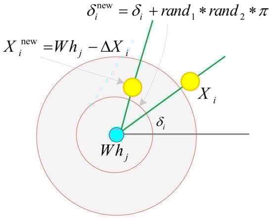
Figure 1. The model by whirlpool for optimization purposes.

According to Figure 1, the objects and particles (X) move around the whirlpool center at a special angle (δ). As a result, the angle varies at each iteration of the algorithm as: ${\delta }_i^{new}={\delta }_i+ran{d}_1\ast ran{d}_2\ast \pi$.

For ∆X_i, the furthest and nearest whirlpools are calculated according to their objective functions, i.e., the maximum and minimum values of Equation (30), and based on the equation Equations (34) and (35), given below and the value of ith particle’s angle concerning its whirlpool, jth, i.e., δ_i, variation of the particle’s position subject to a reduction in the objective function (describing the particle’s intelligence) is obtained:

$${\mathsf{\Delta }}_t=f\left(W{h}_t \right)\ast {\left|\mathrm{sum}\left(W{h}_t \right)-\mathrm{sum}\left(X_i \right)\right|}^{0.5}$$

(30)

$$\mathsf{\Delta }{X}_i=\left(1+\left|\cos \left({\delta }_i^{new}\right)-\sin \left({\delta }_i^{new}\right) \right|\right)\ast \left(\cos \left({\delta }_i^{new}\right)\ast \left(W{h}_f-X_i\right)-\sin \left({\delta }_i^{new}\right)\ast \left(W{h}_w-X_i\right)\right)$$

(31)

$$X_i^{new}=W{h}_j-\Delta X_i$$

(32)

where $W{h}_f$ is $Wh$ with a minimum value of ${\mathsf{\Delta }}_t$ and $W{h}_w$ is $Wh$ with a maximum value of ${\mathsf{\Delta }}_t$, respectively. The pseudo-code of generating a new position can be summarized given in Algorithm 1.

Algorithm 1. Generating the new position (Pseudo-code 1)
1:	for $t=1\text{:}{N}_{Wh}-\left\{j\right\}$
2:	Calculate ${\mathsf{\Delta }}_t$ using Equation (30)
3:	end
4:	$W{h}_f=Wh$ with the minimum value of ${\mathsf{\Delta }}_t$
5:	$W{h}_w=Wh$ with the maximum value of ${\mathsf{\Delta }}_t$
6:	${\delta }_i^{new}={\delta }_i+ran{d}_1\ast ran{d}_2\ast \pi$
7:	Calculate $\Delta X_i$ using Equation (31)
8:	$X_i^{new}=W{h}_j-\mathsf{\Delta }{X}_i$

Then, the new position can be updated using the pseudo-code provided in Algorithm 2.

Algorithm 2. Updating the new position (Pseudo-code 2)
1:	$X_i^{new}=\min \left(\max \left(X_i^{new},X^{min}\right),X^{max}\right)$
2:	if $f\left(X_i^{new}\right)<=f\left(X_i\right)$
3:	$X_i=X_i^{new}$
4:	$f\left(X_i\right)=f\left(X_i^{new}\right)$
5:	end

3.1.3. Centrifugal Force

Centripetal force drags the moving objects into the center, but centrifugal force acts the opposite. Centrifugal force (or FE_i) may be greater than the FE_i of Wh and move particles randomly to novel positions. Centrifugal force is modeled in Equation (33). This is performed so that FE_i is found according to its angle with the center of the whirlpool. In the case the FE_i is greater than a random value of r, the centrifugal attraction and drag apply randomly on the chosen pth dimension as given here:

$$F{E}_i={\left({\left(\cos \left({\delta }_i^{new}\right)\right)}^2\ast {\left(\sin \left({\delta }_i^{new}\right)\right)}^2\right)}^2$$

(33)

$$x_{i,p}\left(t\right)=x_p^{min}+x_p^{max}-x_{i,p}\left(t-1\right)$$

(34)

Algorithm 3 summarized he pseudo-code of this process.

Algorithm 3. Updating pth position using the centrifugal force (Pseudo-code 3)
1:	Evaluate the centrifugal force ($F{E}_i)$ using Equation (33)
2:	$if rand<F{E}_i$
3:	$p=\mathrm{round}\left(1+\mathrm{rand}\ast \left(D-1\right)\right);$
4:	Update $x_{i,p}$ using Equation (34)
5:	$f\left(X_i\right)=f\left(X_i^{new}\right)$
6:	end

This is expressed as shown in Figure 2.

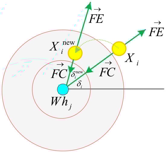
Figure 2. Acting forces in whirlpools.

3.1.4. Interactions between Whirlpools

To model and calculate ∆Wh_j, the objective function and minimum value of Equation (35) are used to calculate the nearest whirlpool, and according to the Equations (36) and (37) given in the following and based on the value of the jth whirlpool’s angle, δ_j, variation of the whirlpool’s position subject to the reduction in its objective function (artificial intelligence) is obtained.

$${\Delta }_t=f\left(W{h}_t \right)\ast \left|\mathrm{sum}\left(W{h}_t \right)-\mathrm{sum}\left(W{h}_j \right)\right|$$

(35)

$$\Delta W{h}_j=rand\left(1,D\right)\ast \left|\cos \left({\delta }_j^{new}\right)+\sin \left({\delta }_j^{new}\right) \right|\ast \left(W{h}_f-W{h}_j\right)$$

(36)

$$W{h}_j^{new}=W{h}_f-\Delta W{h}_j$$

(37)

Algorithm 4 presents the pseudo-code of this phase.

Algorithm 4. Whirlpools’ interaction process (Pseudo-code 4)
1:	for$t=1: N\_Wh-\left\{j\right\}$
2:	Calculate ${\Delta }_t$ using Equation (35)
3:	$\mathbf{end}$
4:	$W{h}_f=Wh$ with the minimum value of ${\mathsf{\Delta }}_t$
5:	Evaluate $\Delta W{h}_j$ using Equation (36)
6:	$W{h}_j^{new}=W{h}_f-\Delta W{h}_j$
7:	${\delta }_j^{new}={\delta }_j+ran{d}_1\ast ran{d}_2\ast \pi$

Updating mechanism whirlpools is illustrated in Algorithm 5.

Algorithm 5. Whirlpools’ updating process (Pseudo-code 5)
1:	$W{h}_j^{new}=\min \left(\max \left(W{h}_j^{new},X^{min}\right),X^{max}()\right)$
2:	$iff\left(W{h}_j^{new}\right)<=f\left(W{h}_j\right)$
3:	$W{h}_j=W{h}_j^{new}$
4:	$f\left(W{h}_j\right)=f\left(W{h}_j^{new}\right)$
5:	$end$

Subsequently, provided that the most potent member within new elements of the whirlpool’s set is stronger and/or the objective function is smaller than the center and hole of the whirlpool, it is chosen as the new center and hole of the whirlpool for the next iteration, and the role of this most vital new member is replaced with the previous center and well of the whirlpool, as shown in Algorithm 6.

Algorithm 6. Selection mechanism (Pseudo-code 6)
1:	$if f\left(X_{best }\right)<=f\left(W{h}_j \right)$
2:	$W{h}_j\leftrightarrow X_{best }$
3:	$f\left(W{h}_j\right)\leftrightarrow f\left(X_{best }\right)$
4:	$end$

Figure 3 illustrates the step-by-step procedure of the TFWO algorithm.

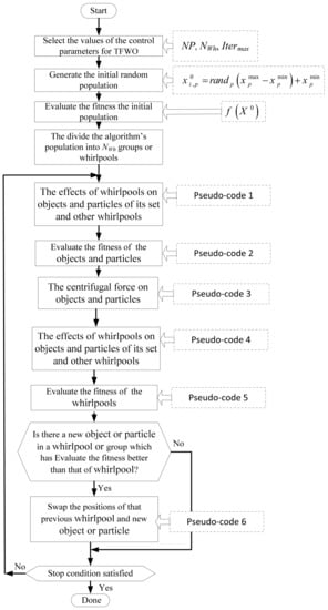
Figure 3. Flowchart of the original TFWO.

3.2. TLBO Algorithm

This method was presented in 2012 by Rao et al., which is similar to other optimization methods derived from nature, is based on population, and refers to the influence of a teacher on student learning in the classroom. The TLBO algorithm takes advantage of the students’ learning ability in the classroom and the teacher’s teaching to improve the class’s academic level. The teacher and the students are the two main elements of the algorithm. In iteration i, the teacher (Ti) attempts to increase the student’s academic level and bring them to their academic level, which can be achieved by improving the students’ average from the value Mi to the value Mi + 1 in the next iteration. Because the students’ level in the first iteration increases with the teacher’s training, a new teacher is selected for the next iteration to provide further training to the students to advance the education process. This new teacher in the new iteration (i + 1) is selected from among the students in the new iteration as a selection among the best member (Ti + 1).

In this algorithm, first, an initial population is determined with the size of swarm Np and the size of design parameters D equal to the number of structural elements. Suppose this population is considered a matrix. In that case, the population of the class is defined according to the Equation (1) of the matrix with Npop rows and D columns.

$$\left[\begin{array}{c}{X}_{11},X_{12},\dots ,X_{1D}\\ X_{21},X_{22},\dots ,X_{2D}\\ ⋮\\ X_{Npop1},X_{Npop2},\dots ,X_{NpopD}\end{array}\right]$$

(38)

3.2.1. Teaching Phase

In this phase, the member with the best value (minimum response value for weight) is chosen from the population as the teacher. Then, the following equation is applied to each of the students (e.g., to the ith student):

$$X_i^{new}=X_i+\Delta X_i$$

(39)

Parameter $\mathsf{\Delta }{X}_i$ is the movement step and the difference between the teacher and class mean. It should be selected, so students’ knowledge is transferred to the teacher. This parameter is calculated as follows:

$$\mathsf{\Delta }{X}_i=rand\ast \left(Teacher-T_F\ast X_{mean}\right)$$

(40)

Here, $X_{mean}$ is the mean position of all members up to the current iteration of the algorithm and rand is a random variable between 0 and 1 with dimensions equal to the variables of the problem under study. Moreover, $T_F$ is the learning rate, which is either 1 or 2, i.e., $T_F=1+round(rand)$. If, in the above equation, $X_i^{new}$ has a better position than $X_i$, the position of $X_i$ is equal to $X_i^{new}$. Because TLBO is an iteration-based algorithm, the role of the teacher substitutes for that of one of the students at the end of each teaching phase. It is essential to calculate the average to show the search scale. The formulation presented by Rao to calculate the mean value is as follows:

$$X_{mean}=\frac{1}{Npop}{\displaystyle \sum }_{i=1}^{Npop}{X}_i$$

(41)

3.2.2. Learning Phase

This step constitutes the second part of the TLBO algorithm, in which the students enhance their knowledge and information. Each of the students communicates with other students randomly, e.g., with the jth member shown by $X_j$, and if the level of each one is higher, they teach lessons to the other student to enhance their status. This process is stated as follows. If the jthe member has a better function value than the ith member:

$$X_i^{new}=X_i+rand\ast \left(X_j-X_i\right)$$

(42)

Otherwise,

$$X_i^{new}=X_i+rand\ast \left(X_i-X_j\right)$$

(43)

If, in the above equation, $X_i^{new}$ has a better position than $X_i$, then the position of $X_i$ will be equal to $X_i^{new}$.

3.3. The Proposed TLTFWO Algorithm

Trapping in the local optima and low accuracy are two major disadvantages of the original TFWO algorithm. The current article presents the TLTFWO algorithm to strengthen the weak points of the TFWO and facilitate information exchange among the population. Each of the members or individuals is constantly communicating with others in other populations. This helps advance the searching step within the search space and prevent trapping in the local optima. Thereby, the performance of the TFWO is remarkably improved, and the TLBO algorithm’s ability to search the decision space is enhanced, as well as its exploitation potential.

Equation (44) describes the modified and improved searching process in the hybrid TLTFWO algorithm. In this equation, $W{h}_f$ and $W{h}_w$ are used in the learning phase of the ith particle and the whirlpool to which ith particle belongs, i.e., $W{h}_j$, is adopted for the teaching phase. In this equation, it moves towards the global and local optima and between them based on different movement equations and different accelerations so that the searching range is somehow improved, and this leads to the algorithm effectively avoiding from trapping in the local optima. This new equation helps enhance local and global searching potential and thus reaches the final solution.

$$\begin{array}{l}\mathsf{\Delta }{X}_i=\left(1+\left|\cos \left({\delta }_i^{new}\right)-\sin \left({\delta }_i^{new}\right)\right|\right)\\ \ast \left(\cos \left({\delta }_i^{new}\right)\ast \left(W{h}_j-T_F\ast X_{mean }\right)-\sin \left({\delta }_i^{new}\right)\ast \left(W{h}_f-W{h}_w\right)\right)\end{array}$$

(44)

$$X_i^{new}=X_i+\mathsf{\Delta }{X}_i$$

(45)

4. TLTFWO for Different OPF Problems

The IEEE 30-bus system is used to test TFWO, TLBO, and TLTFWO algorithms by examining eight cases of OPF problems. The maximum number of iterations is set at 600 in all the algorithms, the TFWO with Npop = 45 (population size) and N_Wh = 3 (number of whirlpools), TLBO with Npop = 30, and TLTFWO with Npop = 45 and N_Wh = 3. Power systems parameters are given in [56]. MATLAB 8.3 (R2014a) is adopted for simulations in a PC with a Corei7 CPU 3.0 GHz and 8.0 GB RAM configuration.

4.1. OPF Solutions IEEE 30-Bus Network [56]

As demonstrated in Figure 4 [56], the active and reactive demand of the test system are 283.4 MW and 126.2 MVAr, respectively.

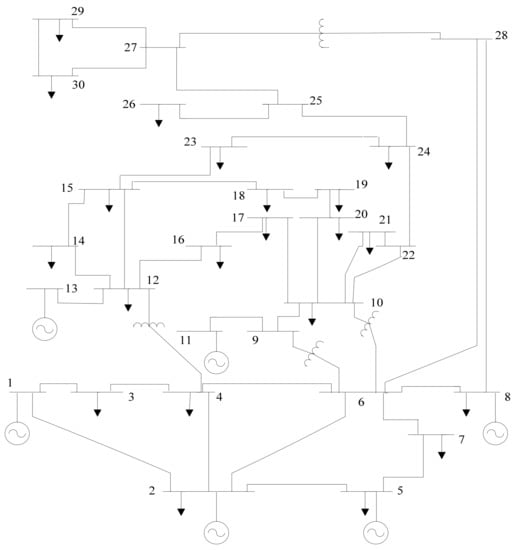
Figure 4. The layout of the IEEE 30-bus system.

The capability of the suggested TLTFWO algorithm is demonstrated by applying six OPF cases to the test system (without WT and PV). The objective functions are the same as in Section 2. Table 3 reports the optimal results found by the algorithm as the best values for thirty runs on each case. The results are compatible with the assumed objective functions, where all limits are observed.

Table 3. Optimal values of the OPF problem variables without stochastic renewable energy, obtained by TLTFWO.

Parameters	Cases:
	1	2	3	4	5	6
PG1	177.1398	139.9991	198.7424	102.6131	176.2434	122.1760
PG2	48.7069	55.0000	44.8704	55.5533	48.8509	52.5571
PG5	21.3886	24.0889	18.4725	38.1107	21.6373	31.4806
PG8	21.2540	34.9994	10.0001	35.0000	22.2667	35.0000
PG11	11.9311	18.3672	10.0000	30.0000	12.2386	26.7497
PG13	12.0000	17.6834	12.0002	26.6524	12.0008	21.0234
VG1	1.0839	1.0744	1.0816	1.0698	1.0421	1.0731
VG2	1.0607	1.0572	1.0581	1.0576	1.0226	1.0574
VG5	1.0340	1.0312	1.0309	1.0359	1.0137	1.0327
VG8	1.0383	1.0392	1.0372	1.0438	1.0057	1.0409
VG11	1.0996	1.0869	1.0986	1.0835	1.0732	1.0402
VG13	1.0513	1.0666	1.0629	1.0573	0.9875	1.0244
T6–9	1.0707	1.0249	1.0412	1.0857	1.0998	1.0999
T6–10	0.9183	0.9590	0.9730	0.9000	0.9001	0.9512
T4–12	0.9762	1.0015	0.9952	0.9901	0.9385	1.0326
T28–27	0.9737	0.9731	0.9782	0.9750	0.9711	1.0047
QC10	2.4939	3.6587	4.5988	4.5252	4.9938	3.1650
QC12	1.0909	0.0003	1.9342	0.1672	0.0542	0.0312
QC15	4.4547	3.9139	4.3825	4.4646	4.9993	3.8300
QC17	5.0000	5.0000	4.9907	5.0000	0	4.9997
QC20	4.2352	4.2499	4.3793	4.2524	5.0000	4.9999
QC21	5.0000	5.0000	4.9994	5.0000	4.9981	5.0000
QC23	3.2543	3.3075	3.1515	3.2616	4.9980	4.2227
QC24	5.0000	5.0000	4.9987	5.0000	4.9999	5.0000
QC29	2.6470	2.6285	2.6856	2.5559	2.6457	2.6067
Cost (USD/h)	800.4780	646.4715	832.1584	859.0075	803.6829	830.2863
Emission (t/h)	0.3663	0.2835	0.4378	0.2289	0.3636	0.2529
Power losses (MW)	9.0204	6.7380	10.6856	4.5295	9.8377	5.5868
V.D. (p.u.)	0.9084	0.9152	0.8618	0.9279	0.0950	0.2976

4.1.1. Case 1: Minimization of Fuel Cost

In Case 1, the fuel cost of all generating units is minimized as in Equation (46):

$$\begin{array}{l}J={\displaystyle \sum _{i=1}^{NG}({\alpha }_i+b_i{P}_{Gi}+c_i{P}_{Gi}^2)}+{\lambda }_P(P_{G1}-P_{G1}^{\lim }{)}^2+{\lambda }_V{\displaystyle \sum _{i=1}^{NL}{(V{L}_i-V{L}_i^{\lim })}^2}\\ +{\lambda }_Q{\displaystyle \sum _{i=1}^{NG}{(Q_{Gi}-Q_{Gi}^{\lim })}^2}+{\lambda }_S{\displaystyle \sum _{i=1}^{NTL}{(S_i-S_i^{\lim })}^2}\end{array}$$

(46)

Simulation results, shown in Table 3, illustrate that the fuel cost when applying the TLTFWO is 800.4780 (USD/h), which is less compared with those of the results reported in the literature and novel optimization approaches listed in Table 4, such as tabu search (TS) [57], artificial bee colony (ABC) [58], hybrid shuffle frog leaping algorithm (SFLA) and simulated annealing (SFLA-SA) [59], differential evolution (DE) [60], adaptive group search optimization (AGSO) [61], MSA [56], GWO [62], evolutionary programming (EP) [63], modified Gaussian bare-bones imperialist competitive algorithm (MGBICA) [64], Aquila optimizer (AO) [65], hybrid particle swarm optimization (PSO) and GSA (gravitational search algorithm) (PSOGSA) [66], hybrid of imperialist competitive algorithm (ICA) and TLBO (teaching-learning-based optimization) (MICA–TLA) [67], adaptive real coded biogeography-based optimization (ARCBBO) [68], a modified honey bee mating optimization (MHBMO) [9], manta ray foraging optimization (MRFO) [69], flower pollination algorithm (FPA) [56], stud krill herd algorithm (SKH) [70], an improved EP (IEP) [71], hybrid firefly algorithm (FA) and JAYA (HFAJAYA) [72], JAYA [73], firefly algorithm (FA) [72], moth-flame optimization (MFO) [56], hybrid phasor PSO (PPSO) and GSA (PPSOGSA) [55], hybrid modified PSO (MPSO) and SFLA (MPSO-SFLA) [11], teaching-learning-based optimization (TLBO), and TFWO. Figure 5 illustrates the convergence of the objective function.

Table 4. Optimal results of the current research in Case 1.

Optimizer	Fuel cost (USD/h)	Emission (t/h)	Power Losses (MW)	V.D. (p.u.)
TS [57]	802.29	-	-	-
ABC [58]	800.660	0.365141	9.0328	0.9209
SFLA-SA [59]	801.79	-	-	-
DE [60]	802.39	-	9.466	-
AGSO [61]	801.75	0.3703	-	-
MSA [56]	800.5099	0.36645	9.0345	0.90357
GWO [62]	801.41	-	9.30	-
EP [63]	803.57	-	-	-
MGBICA [64]	801.1409	0.3296	-	-
AO [65]	801.83	-	-	-
PSOGSA [66]	800.49859	-	9.0339	0.12674
MICA-TLA [67]	801.0488	-	9.1895	-
ARCBBO [68]	800.5159	0.3663	9.0255	0.8867
MHBMO [9]	801.985	-	9.49	-
MRFO [69]	800.7680	-	9.1150	-
FPA [56]	802.7983	0.35959	9.5406	0.36788
SKH [70]	800.5141	0.3662	9.0282	-
IEP [71]	802.46	-	-	-
HFAJAYA [72]	800.4800	0.3659	9.0134	0.9047
JAYA [73]	800.4794	-	9.06481	0.1273
FA [72]	800.7502	0.36532	9.0219	0.9205
MFO [56]	800.6863	0.36849	9.1492	0.75768
PPSOGSA [55]	800.528	-	9.02665	0.91136
MPSO-SFLA [11]	801.75	-	9.54	-
TFWO	800.8426	0.3668	9.3207	0.9044
TLBO	800.9923	0.3369	9.4892	0.9026
TLTFWO	800.4780	0.3663	9.0204	0.9084

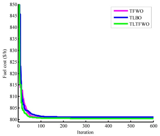
Figure 5. Convergence trends for Case 1.

4.1.2. Case 2: Minimization of Piecewise Quadratic Fuel Cost

Several thermal generating units can utilize fuel sources such as oil, coal or natural gas. The fuel cost coefficients of generators operating with a single fuel type are similar to those of Case 1. The fuel cost characteristics of the units located at buses 1 and 2 are expressed as:

$$f_i(P_{Gi})={\displaystyle \sum _{k=1}^{n_f}{\alpha }_{i,k}+b_{i,k}{P}_{Gi}+c_{i,k}{P}_{Gi}^2}$$

(47)

where nf denotes the number of fossil fuel alternatives for the ith generating unit, and a_i,k, b_i,k, and c_i,k are cost coefficients of generating unit i when the kth fuel is the alternative.

The objective function can be described by Equation (42).

$$\begin{array}{l}{J}_2={\displaystyle \sum _{k=1}^{NG}{\alpha }_{i,k}+b_{i,k}{P}_{Gi}+c_{i,k}{P}_{Gi}^2}+{\lambda }_P(P_{G1}-P_{G1}^{\lim }{)}^2+{\lambda }_V{\displaystyle \sum _{i=1}^{NL}{(V{L}_i-V{L}_i^{\lim })}^2}\\ +{\lambda }_Q{\displaystyle \sum _{i=1}^{NG}{(Q_{Gi}-Q_{Gi}^{\lim })}^2}+{\lambda }_S{\displaystyle \sum _{i=1}^{NTL}{(S_i-S_i^{\lim })}^2}\end{array}$$

(48)

According to Table 3, the fuel cost when the suggested algorithm is applied is 646.4715 (USD/h). The best result belongs to the hybrid TLTFWO algorithm when compared with the results of other techniques listed in Table 5, such as MSA [56], gbest guided ABC (GABC) [74], MFO [56], MPSO-SFLA [11], FPA [56], Lévy TLBO (LTLBO) [4], social spider optimization (SSO) [14], a modified DE (MDE) [60], sparrow search algorithm (SSA) [75], an improved EP (IEP) [71], MICA-TLA [67], TLBO, and TFWO, where the TLTFWO provides best fuel cost than the reported results in the literature. Moreover, Figure 6 demonstrates the convergence behavior of the algorithms when applied to the OPF problem with minimum fuel cost (USD/h).

Table 5. The optimal results found by different algorithms in Case 2.

Optimizer	Fuel cost (USD/h)	Emission (t/h)	Power Losses (MW)	V.D. (p.u.)
MSA [56]	646.8364	0.28352	6.8001	0.84479
GABC [74]	647.03	-	6.8160	0.8010
MFO [56]	649.2727	0.28336	7.2293	0.47024
MPSO-SFLA [11]	647.55	-	-	-
FPA [56]	651.3768	0.28083	7.2355	0.31259
LTLBO [4]	647.4315	0.2835	6.9347	0.8896
SSO [14]	663.3518	-	-	-
MDE [60]	647.846	-	7.095	-
SSA [75]	646.7796	0.2836	6.5599	0.5320
IEP [71]	649.312	-	-	-
MICA-TLA [67]	647.1002	-	6.8945	-
TFWO	646.9425	0.2840	6.8026	0.9136
TLBO	647.5263	0.2838	6.8375	0.9102
TLTFWO	646.4715	0.2835	6.7380	0.9152

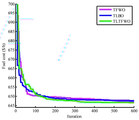
Figure 6. Convergence trends for Case 2.

4.1.3. Case 3: Minimization of Fuel Cost Considering VPEs

To consider the impact of loading on the performance of generating units, this part of the article adds a new (sinusoidal) term in the cost functions of generating units so that vale point effects (VPEs) behavior is imitated.

The VPEs are involved in the cost function as Equation (49).

$$\begin{array}{l}{J}_3={\displaystyle \sum _{i=1}^{NG}{\alpha }_i+b_i{P}_{Gi}+c_i{P}_{Gi}^2+\left|e_i\sin \left(f_i\left(P_{Gi}^{\min }-P_{Gi}\right)\right)\right|}+{\lambda }_P(P_{G1}-P_{G1}^{\lim }{)}^2+{\lambda }_V{\displaystyle \sum _{i=1}^{NL}{(V{L}_i-V{L}_i^{\lim })}^2}\\ +{\lambda }_Q{\displaystyle \sum _{i=1}^{NG}{(Q_{Gi}-Q_{Gi}^{\lim })}^2}+{\lambda }_S{\displaystyle \sum _{i=1}^{NTL}{(S_i-S_i^{\lim })}^2}\end{array}$$

(49)

Here e_i and f_i show the valve point cost coefficients of the ith unit.

Table 3 and Table 6 tabulate the optimal settings of control variables of the suggested approach, where a comparison is made between the TLTFWO and its counterparts. The suggested method achieves the minimum fuel cost, which is 832.1584 (USD/h). Further, the algorithm helps reach the most suitable OPF solutions as per the obtained results. The convergence curves of the TFWO, TLBO and TLTFWO algorithms in Case 3 are shown in Figure 7.

Table 6. Optimal results found by the TLTFWO in Case 3.

Optimizer	Fuel Cost (USD/h)	Emission (t/h)	Power Losses (MW)	V.D. (p.u.)
HFAJAYA [72]	832.1798	0.4378	10.6897	0.8578
FA [72]	832.5596	0.4372	10.6823	0.8539
SP-DE [76]	832.4813	0.43651	10.6762	0.75042
PSO [77]	832.6871	-	-	-
TFWO	832.6598	0.4382	10.9105	0.8410
TLBO	832.7624	0.4380	10.9397	0.8322
TLTFWO	832.1584	0.4378	10.6856	0.8618

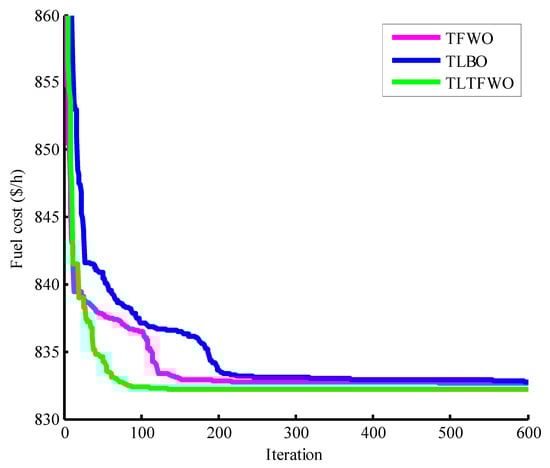
Figure 7. Convergence trends in Case 3.

In cases 4 to 6, the TLTFWO algorithm is applied to find more suitable solutions to multi-objective OPF problems. Moreover, the best simulation solutions found by the TLTFWO in cases 4 to 6 are listed in Table 3.

4.1.4. Case 4: Minimization of Real Power Loss and Fuel Cost

Here, the performance of the TLTFWO algorithm is assessed, where the objective function is formulated such that the quadratic cost function and active power loss are minimized based on Equations (16) and (17). Thirty tests are executed in simulations to solve the OPF problem repetitively using TLTFWO. Equation (50) gives the objective function of OPF:

$$\begin{array}{l}{J}_4={\displaystyle \sum _{i=1}^{NG}{\alpha }_i+b_i{P}_{Gi}+c_i{P}_{Gi}^2}+{\varphi }_p{\displaystyle \sum _{i=1}^{NTL}{\displaystyle \sum _{\begin{array}{l}j=1\\ j\ne i\end{array}}^{NTL}{G}_{ij}{V}_i^2+B_{ij}{V}_j^2-2V_i{V}_j\cos {\delta }_{ij}}}+{\lambda }_P(P_{G1}-P_{G1}^{\lim }{)}^2\\ +{\lambda }_V{\displaystyle \sum _{i=1}^{NL}{(V{L}_i-V{L}_i^{\lim })}^2}+{\lambda }_Q{\displaystyle \sum _{i=1}^{NG}{(Q_{Gi}-Q_{Gi}^{\lim })}^2}+{\lambda }_S{\displaystyle \sum _{i=1}^{NTL}{(S_i-S_i^{\lim })}^2}\end{array}$$

(50)

here ${\varphi }_p$ = 40 is set, similar to [56].

Table 3 shows the optimal settings of control variables. Additionally, the convergence behavior of the best result obtained for fuel cost from the implemented algorithm can be provided in Figure 8. Table 7 compares the performance of the proposed TLTFWO algorithm with some other techniques already mentioned throughout the article. The values of fuel cost and active power loss in the case of utilizing the proposed method are 859.0075 (USD/h) and 4.5295 (MW), respectively.

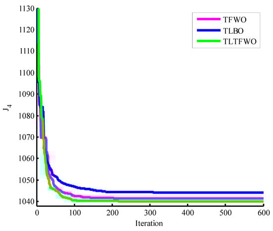
Figure 8. Convergence trends for Case 4.

Table 7. Optimal results of the present study in Case 4.

Optimizer	Fuel Cost (USD/h)	Emission (t/h)	Power Losses (MW)	V.D. (p.u.)	${\mathit{J}}_4$
EMSA [78]	859.9514	0.2278	4.6071	0.7758	1044.2354
MOALO [13]	826.4556	0.2642	5.7727	1.2560	1057.3636
MJaya [79]	827.9124	-	5.7960	-	1059.7524
MSA [56]	859.1915	0.2289	4.5404	0.92852	1040.8075
SpDEA [80]	837.8510	-	5.6093	0.8106	1062.223
QOMJaya [79]	826.9651	-	5.7596	-	1402.9251
TFWO	860.1514	0.2292	4.5335	0.9145	1041.4914
TLBO	860.2684	0.2295	4.6002	0.9096	1044.2764
TLTFWO	859.0075	0.2289	4.5295	0.9279	1040.1875

According to Table 5, one can understand that the overall objective function found by the TLTFWO is significantly smaller than those of the previous research reports.

4.1.5. Case 5: Minimization of Fuel Cost and Voltage Deviation

Among the critical indices of network security and continuation of supply to the customers is the magnitude of voltages of network buses. It is worth noting that adopting only one cost objective function in the OPF problem reaches a solution in which the voltage profile is unsatisfying. To this end, the present problem utilizes two objective functions: the fuel cost is minimized, the voltage profile is enhanced, and the voltage deviation on load buses does not violate one p.u. Equation (51) formulates the objective function of Case 5:

$$\begin{array}{l}{J}_5={\displaystyle \sum _{i=1}^{NG}{\alpha }_i+b_i{P}_{Gi}+c_i{P}_{Gi}^2}+{\varphi }_v{\displaystyle \sum _{i=1}^{NL}\left|V{L}_i-1.0\right|}+{\lambda }_P(P_{G1}-P_{G1}^{\lim }{)}^2\\ +{\lambda }_V{\displaystyle \sum _{i=1}^{NL}{(V{L}_i-V{L}_i^{\lim })}^2}+{\lambda }_Q{\displaystyle \sum _{i=1}^{NG}{(Q_{Gi}-Q_{Gi}^{\lim })}^2}+{\lambda }_S{\displaystyle \sum _{i=1}^{NTL}{(S_i-S_i^{\lim })}^2}\end{array}$$

(51)

where, ${\varphi }_v$ = 100 [56].

Table 3 provides the results of optimal settings of control variables when the TLTFWO is used for simulations. In addition, Table 8 compares the results of various algorithms. As is observed, TLTFWO has significantly reduced the value of the multi-objective function. The convergence curves of this function obtained by the TFWO, TLBO and TLTFWO algorithms in Case 5 are shown in Figure 9.

Table 8. Optimal results of the present study in Case 5.

Optimizer	Fuel Cost (USD/h)	Emission (t/h)	Power Losses (MW)	V.D. (p.u.)	${\mathit{J}}_5$
PSO [81]	804.477	0.368	10.129	0.126	817.0770
PSO-SSO [81]	803.9899	0.367	9.961	0.0940	813.3899
BB-MOPSO [82]	804.9639	-	-	0.1021	815.1739
EMSA [78]	803.4286	0.3643	9.7894	0.1073	814.1586
TFWO [17]	803.416	0.365	9.795	0.101	813.5160
SpDEA [80]	803.0290	-	9.0949	0.2799	831.0190
MFO [56]	803.7911	0.36355	9.8685	0.10563	814.3541
DA-APSO [83]	802.63	-	-	0.1164	814.2700
SSO [81]	803.73	0.365	9.841	0.1044	814.1700
MOMICA [82]	804.9611	0.3552	9.8212	0.0952	814.4811
MPSO [56]	803.9787	0.3636	9.9242	0.1202	815.9987
MNSGA-II [82]	805.0076	-	-	0.0989	814.8976
TFWO	804.2510	0.3639	10.1563	0.0998	814.2310
TLBO	804.7380	0.3671	9.9995	0.1065	815.3880
TLTFWO	803.6829	0.3636	9.8377	0.09450	813.1829

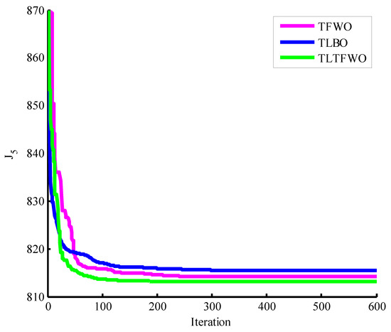
Figure 9. Convergence trends in Case 5.

4.1.6. Case 6: Minimization of Fuel Cost, Emissions, Voltage Deviation and Losses

This study deals with two types of pollutant gases emitted from generating units, SO_x and NO_x. By assigning appropriate coefficients for their price, attempts to minimize the tota amoutn of emission as given in Equation (25). This equations attempts to find minimum values of fuel cost, votage deviation, pollutant level, and power loss at the same time:

$$\begin{array}{cc}\hfill & J_6=\sum _{i=1}^{NG}{\alpha }_i+b_i{P}_{Gi}+c_i{P}_{Gi}^2+{\varphi }_p\sum _{i=1}^{NTL}\sum _{\begin{array}{c}j=1\\ j\ne i\end{array}}^{NTL}{G}_{ij}{V}_i^2+B_{ij}{V}_j^2-2V_i{V}_{j}cos{\delta }_{ij}+{\varphi }_v\sum _{i=1}^{NL}\left|V{L}_i-1.0\right|\hfill \\ \hfill & +{\varphi }_{e}min\sum _{i=1}^{NG}\left({\alpha }_i+{\beta }_i{P}_{Gi}+{\gamma }_i{P}_{Gi}^2+{\xi }_{i}exp\left({\theta }_i{P}_{Gi}\right)\right)+{\lambda }_P{(P_{G1}-P_{G1}^{lim})}^2\hfill \\ \hfill & +{\lambda }_V\sum _{i=1}^{NL}{(V{L}_i-V{L}_i^{lim})}^2+{\lambda }_Q\sum _{i=1}^{NG}{(Q_{Gi}-Q_{Gi}^{lim})}^2+{\lambda }_S\sum _{i=1}^{NTL}{(S_i-S_i^{lim})}^2\hfill \end{array}$$

(52)

The present paper adopts ${\varphi }_v$ = 21, ${\varphi }_p$ = 22 and ${\varphi }_e$ = 19 [56] as the weight coefficients.

Once again, the TLTFWO algorithm demonstrates its potential to deal with the formulated optimization problem. Table 9 lists the results of different algorithms when applied to the problem.

Table 9. Optimal results of the present study in Case 6.

Algorithm	Fuel Cost (USD/h)	Emission (t/h)	Power Losses (MW)	V.D. (p.u.)	${\mathit{J}}_6$
SSO [81]	829.978	0.25	5.426	0.516	964.9360
MODA [84]	828.49	0.265	5.912	0.585	975.8740
MNSGA-II [82]	834.5616	0.2527	5.6606	0.4308	972.9429
PSO [81]	828.2904	0.261	5.644	0.55	968.9674
J-PPS3 [85]	830.3088	0.2363	5.6377	0.2949	965.0228
I-NSGA-III [86]	881.9395	0.2209	4.7449	0.1754	994.2078
MFO [56]	830.9135	0.25231	5.5971	0.33164	965.8080
J-PPS2 [85]	830.8672	0.2357	5.6175	0.2948	965.1201
MOALO [13]	826.2676	0.2730	7.2073	0.7160	1005.0512
MSA [56]	830.639	0.25258	5.6219	0.29385	965.2907
BB-MOPSO [82]	833.0345	0.2479	5.6504	0.3945	970.3379
J-PPS1 [85]	830.9938	0.2355	5.6120	0.2990	965.2159
TFWO	831.7219	0.2540	5.6523	0.2981	967.1586
TLBO	831.2634	0.2602	5.8517	0.3111	971.4777
TLTFWO	830.2863	0.2529	5.5868	0.2976	964.2506

As per this table, the minimum value of the objective function is 964.2506, which is smaller than its counterparts. The convergence curve of the total objective function in Case 6 by the TFWO, TLBO, and TLTFWO algorithms is displayed in Figure 10.

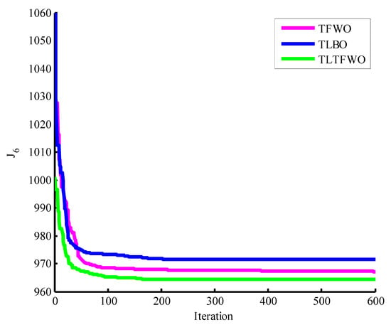
Figure 10. Convergence trends for Case 6.

4.2. OPF Problem Solution in the Presence of WT and PV Units

4.2.1. Case 7: Minimizing the Generation Cost When Incorporating WT and PV Generation

In this case, the TLTFWO helps find the minimum fuel, wind, and PV costs defined by Equation (53) for a system with WT and PV units.

$$\begin{array}{l}{J}_7={\displaystyle \sum _{i=1}^{NG}{\alpha }_i+b_i{P}_{Gi}+c_i{P}_{Gi}^2}+\left({\displaystyle \sum _{i=1}^{NW}F\cos t\left(W{T}_i\right)}\right)+\left({\displaystyle \sum _{i=1}^{NV}F\cos t\left(P{V}_i\right)}\right)\\ {\lambda }_P(P_{G1}-P_{G1}^{\lim }{)}^2+{\lambda }_V{\displaystyle \sum _{i=1}^{NL}{(V{L}_i-V{L}_i^{\lim })}^2}+{\lambda }_Q{\displaystyle \sum _{i=1}^{NG}{(Q_{Gi}-Q_{Gi}^{\lim })}^2}+{\lambda }_S{\displaystyle \sum _{i=1}^{NTL}{(S_i-S_i^{\lim })}^2}\end{array}$$

(53)

NW and NV are the number of WT and PV units in this equation. Further, $F\cos t\left(W{T}_i\right)$ and $F\cos t\left(P{V}_i\right)$ express the output power generation cost of the ith WT and PV units, respectively.

Cost coefficients, in this case, are similar to Case 1, and PDF parameters are given in Table 10. Table 11 provides the optimal solutions of TLTFWO obtained for more than thirty runs. As observed, incorporating the optimal parameters helps decrease the objective function significantly compared to TFWO and TLBO. Moreover, Figure 11 compares convergence behavior in Case 7 between TFWO, TLBO and TLTFWO algorithms.

Table 10. PDF parameters of WT and PV units [19].

Wind Power Generating Plants					Solar PV Plant
Wind Farm	No. of Turbines	Rated Power, Pwr (MW)	Weibull PDF Parameters	Weibull Mean, Mwbl	Rated Power, Psr (MW)	Lognormal PDF Parameters	Lognormal Mean, Mlgn
1 (bus 5)	25	75	c = 9, k = 2	v = 7.976 m/s	50 (bus 13)	σ = 0.6, µ = 6	G = 483 W/m2
2 (bus 11)	20	60	c = 10, k = 2	v = 8.862 m/s

Table 11. Optimal variables in Case 7.

Variables	TFWO	TLBO	TLTFWO
PG1 (MW)	134.90791	134.90791	134.90793
PG2 (MW)	29.0275	28.2868	27.0466
Pws1 (MW)	44.0282	43.6213	42.9326
PG3 (MW)	10	10	10
Pws2 (MW)	37.1649	36.8238	36.2236
Pss (MW)	34.0406	35.5344	38.0833
VG1 (p.u.)	1.0718	1.0723	1.072
VG2 (p.u.)	1.0568	1.0573	1.057
VG5 (p.u.)	1.0349	1.0352	1.0348
VG8 (p.u.)	1.0702	1.0398	1.0395
VG11 (p.u.)	1.0981	1.0996	1.0999
VG13 (p.u.)	1.0489	1.0548	1.0559
QG1 (MVAR)	−2.31923	−1.91971	−1.91987
QG2 (MVAR)	11.8198	13.2443	13.2115
Qws1 (MVAR)	22.4185	23.1879	23.2748
QG3(MVAR)	40	35.0704	34.6188
Qws2 (MVAR)	30	30	30
Qss (MVAR)	15.0849	17.4102	17.8624
Fuelvlvcost (USD/h)	442.3257	439.8602	435.7669
Wind gen cost (USD/h)	247.9662	245.3840	240.9739
Solar gen cost (USD/h)	92.0150	97.2115	105.2384
Total Cost (USD/h)	782.3068	782.4558	781.9791
Emission (t/h)	1.76196	1.76213	1.76245
Power losses (MW)	5.7692	5.7741	5.7941
V.D. (p.u.)	0.45405	0.46348	0.46546

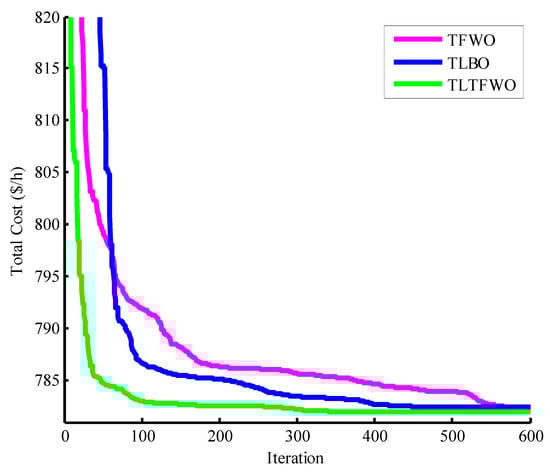
Figure 11. Convergence trends for Case 7.

4.2.2. Case 8: Minimizing Generation Cost in the Presence of WT and PV Units with the Carbon Tax

Carbon tax (C_tax) is assumed on emissions, so the application of clean energy like WT and PV units is encouraged. The emission cost can be mathematically expressed as follows [19]:

$$C_E=C_{tax}E$$

(54)

$$J_8=J_7+C_{tax}E$$

(55)

C_tax is estimated to be USD 20 per tonne [19].

Table 12 lists the OPF results obtained by estimating the output power of WT and PV units while considering a carbon tax. As one can be observed, the suggested TLTFWO gives more suitable solutions and results than both TFWO and TLBO. In the case of applying the carbon tax, both WT and PV units produce higher amounts of output power.

Table 12. The variables’ optimal values obtained for Case 8.

Variables	TFWO	TLBO	TLTFWO
PG1 (MW)	123.11028	123.50416	123.32853
PG2 (MW)	31.9607	33.0291	32.5297
Pws1 (MW)	45.4523	46.0158	45.7041
PG3 (MW)	10	10	10
Pws2 (MW)	38.2959	38.7483	38.5267
Pss (MW)	39.8618	37.4806	38.629
VG1 (p.u.)	1.0696	1.071	1.0697
VG2 (p.u.)	1.0561	1.0514	1.0561
VG5 (p.u.)	1.035	1.1	1.0954
VG8 (p.u.)	1.0686	1.1	1.0402
VG11 (p.u.)	1.1	1.1	1.0985
VG13 (p.u.)	1.0514	1.0594	1.054
QG1 (MVAR)	−3.21843	12.1278	−2.96534
QG2 (MVAR)	10.7334	−20	4.09265
Qws1 (MVAR)	22.2319	35	35
QG3(MVAR)	40	40	32.6276
Qws2 (MVAR)	30	30	30
Qss (MVAR)	15.9599	18.8826	16.9538
Fuelvlvcost (USD/h)	424.8316	429.4076	427.2849
Wind gen cost (USD/h)	256.9048	260.5086	258.6126
Solar gen cost (USD/h)	112.2470	103.7997	107.3181
Total Cost (USD/h)	793.9835	793.7159	793.2156
Emission (t/h)	0.87057	0.89030	0.88144
J8	811.3949	811.5219	810.8444
Power losses (MW)	5.2809	5.3780	5.3180
V.D. (p.u.)	0.46214	0.49157	0.47299
Carbon tax (USD/h)	17.4114	17.806	17.6288

Moreover, Figure 12 illustrates the convergence characteristics of the discussed methods. As is seen, the suggested TLTFWO is superior to other algorithms in terms of convergence to the global optima with less number of iterations than TFWO and TLBO. So, one can choose TLTFWO for more complicated OPF problems when stochastic variables like intermittent output power of WT and PV generating units are considered.

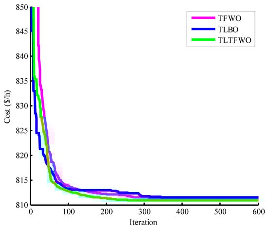
Figure 12. Convergence trends for Case 8.

4.3. Discussions

Table 13 lists the results related to the cost’s minimum, maximum, standard deviation, and mean values. According to this table, the TLTFWO provides more suitable solutions than its counterparts, i.e., PSO [87] (population size = 60), GA [88] (population size= 80), TFWO, and TLBO. Furthermore, even the worst solution of the proposed TLTFWO is more desirable than the best solutions of the PSO, GA, TFWO, and TLBO algorithms. So, TLTFWO is preferred when dealing with OPF problems in reality. Additionally, there is a small difference between the worst, average, and best solutions of the TLTFWO, showing its stability and reliability. The time required to converge to the optimal solution is also acceptable regarding the TLTFWO algorithm.

Table 13. Results of various parameters obtained by TTFWO, TFWO, and TLBO algorithms.

Method	Min	Mean	Max	Std.	Time (s)
Case 1
PSO	801.1419	801.8326	802.9401	1.03	28
GA	801.6345	802.5472	803.2009	1.48	36
TFWO	800.8426	801.2513	801.5878	0.56	30
TLBO	800.9923	801.2958	801.6004	0.45	33
TLTFWO	800.4780	800.6012	800.7639	0.14	30
Case 2
PSO	647.5328	647.9796	648.6117	0.74	31
GA	647.9935	648.7213	649.5020	1.21	35
TFWO	646.9425	647.3011	647.7208	0.42	30
TLBO	647.5263	647.8730	648.4102	0.38	33
TLTFWO	646.4715	646.5819	646.7009	0.17	30
Case 3
PSO	832.9628	833.4139	833.8996	1.01	32
GA	833.6085	834.8323	836.0047	1.95	38
TFWO	832.6598	832.9418	833.3994	0.61	29
TLBO	832.7624	832.9771	833.4825	0.72	34
TLTFWO	832.1584	832.2837	832.4035	0.19	30
Case 4
PSO	1045.3157	1046.7329	1047.3214	1.61	33
GA	1045.9559	1047.1046	1048.3610	1.14	40
TFWO	1041.4914	1042.5326	1043.4218	1.52	31
TLBO	1044.2764	1045.4579	1046.8018	1.49	35
TLTFWO	1040.1875	1040.3267	1040.4793	0.23	29
Case 5
PSO	815.3592	816.5410	817.7862	1.75	32
GA	816.6919	817.7764	819.2102	2.32	35
TFWO	814.2310	815.6249	816.5998	1.40	30
TLBO	815.3880	816.4528	817.6781	1.44	34
TLTFWO	813.1829	813.3613	813.4817	0.15	30
Case 6
PSO	970.9024	973.1466	974.1565	1.39	36
GA	973.4101	975.6303	976.8919	2.16	40
TFWO	967.1586	967.8543	968.4628	0.55	30
TLBO	971.4777	972.0647	972.9847	0.81	33
TLTFWO	964.2506	964.3928	964.5224	0.15	32
Case 7
PSO	782.7100	783.2148	783.7969	0.89	33
GA	783.2565	784.6206	786.7536	1.37	41
TFWO	782.3068	782.6754	783.2645	0.63	35
TLBO	782.4558	782.9740	783.8231	0.94	38
TLTFWO	781.9791	782.2216	782.4136	0.20	35
Case 8
PSO	811.4062	812.5325	813.5510	0.57	33
GA	812.6163	813.7541	815.4792	2.25	40
TFWO	811.3949	812.3127	813.1720	1.16	35
TLBO	811.5219	812.3812	813.2546	1.43	39
TLTFWO	810.8444	810.9632	811.2148	0.18	35

Moreover, the first benefit of using renewable energy sources can be understood by comparing the fuel cost calculated in the two studied cases, 1 and 7. The optimized calculation cost in case 1 for the proposed algorithm equals 800.4780 USD/h. In contrast, the value of the fuel cost calculated in case 7 of the article for the same system with renewable energy is equal to 781.9791 USD/h, which has a significant reduction. On the other hand, with the optimal use of renewable energy sources in the energy system, pollution can be effectively reduced. For example, by comparing cases 7 and 8, it can be seen that by considering the amount of production pollution as an objective function, the amount of pollution has been reduced effectively. For the proposed algorithm, it has decreased from the value of 1.76245 t/h to a much lower value and almost half equal to 0.88144 t/h. If we had used fossil fuel sources instead of these renewable energy production units, we would never have been able to reduce the amount of production pollution to this extent.

5. Conclusions

The current article combined TFWO and TLBO algorithms to introduce a novel optimization algorithm named TLTFWO. The OPF problem was then formulated as a nonlinear optimization problem with some constraints and limits. To improve voltage profile and reduce the fuel cost as much as possible, various objective functions are expressed while considering the impact of the valve point and the presence of PV and WT generating units. The simulations are implemented on the IEEE 30-bus network. According to the findings, the TLTFWO algorithm shows promising performance by successfully solving the multi-objective OPF problem. Simulations prove the robustness of TLTFWO in reaching the optimum global point with optimal adjustments of control variables. The suggested approach can be adopted as the desired tool to address complex power systems and experience more updates and improvements in the upcoming years.

References

- Pourakbari-Kasmaei, M.; Mantovani, J.R.S. Logically constrained optimal power flow: Solver-based mixed-integer nonlinear programming model. Int. J. Electr. Power Energy Syst. 2018, 97, 240–249. [Google Scholar] [CrossRef]
- Momoh, J.A.; Adapa, R.; El-Hawary, M.E. A review of selected optimal power flow literature to 1993. I. Nonlinear and quadratic programming approaches. IEEE Trans. Power Syst. 1999, 14, 96–104. [Google Scholar] [CrossRef]
- Momoh, J.A.; El-Hawary, M.E.; Adapa, R. A review of selected optimal power flow literature to 1993. II. Newton, linear programming and interior point methods. IEEE Trans. Power Syst. 1999, 14, 105–111. [Google Scholar] [CrossRef]
- Ghasemi, M.; Ghavidel, S.; Gitizadeh, M.; Akbari, E. An improved teaching–learning-based optimization algorithm using Lévy mutation strategy for non-smooth optimal power flow. Int. J. Electr. Power Energy Syst. 2015, 65, 375–384. [Google Scholar] [CrossRef]
- Dasgupta, K.; Roy, P.K.; Mukherjee, V. Power flow based hydro-thermal-wind scheduling of hybrid power system using sine cosine algorithm. Electr. Power Syst. Res. 2020, 178, 106018. [Google Scholar] [CrossRef]
- Attia, A.-F.; el Sehiemy, R.A.; Hasanien, H.M. Optimal power flow solution in power systems using a novel Sine-Cosine algorithm. Int. J. Electr. Power Energy Syst. 2018, 99, 331–343. [Google Scholar] [CrossRef]
- Güçyetmez, M.; Çam, E. A new hybrid algorithm with genetic-teaching learning optimization (G-TLBO) technique for optimizing of power flow in wind-thermal power systems. Electr. Eng. 2016, 98, 145–157. [Google Scholar] [CrossRef]
- Pham, L.H.; Dinh, B.H.; Nguyen, T.T. Optimal power flow for an integrated wind-solar-hydro-thermal power system considering uncertainty of wind speed and solar radiation. Neural Comput. Appl. 2022, 34, 10655–10689. [Google Scholar] [CrossRef]
- El-Fergany, A.A.; Hasanien, H.M. Single and Multi-objective Optimal Power Flow Using Grey Wolf Optimizer and Differential Evolution Algorithms. Electr. Power Compon. Syst. 2015, 43, 1548–1559. [Google Scholar] [CrossRef]
- Maheshwari, A.; Sood, Y.R. Solution approach for optimal power flow considering wind turbine and environmental emissions. Wind Eng. 2022, 46, 480–502. [Google Scholar] [CrossRef]
- Narimani, M.R.; Azizipanah-Abarghooee, R.; Zoghdar-Moghadam-Shahrekohne, B.; Gholami, K. A novel approach to multi-objective optimal power flow by a new hybrid optimization algorithm considering generator constraints and multi-fuel type. Energy 2013, 49, 119–136. [Google Scholar] [CrossRef]
- Duman, S.; Wu, L.; Li, J. Moth swarm algorithm based approach for the ACOPF considering wind and tidal energy. In The International Conference on Artificial Intelligence and Applied Mathematics in Engineering; Springer: Cham, Switzerland, 2019; pp. 830–843. [Google Scholar]
- Herbadji, O.; Slimani, L.; Bouktir, T. Optimal power flow with four conflicting objective functions using multi-objective ant lion algorithm: A case study of the algerian electrical network. Iran. J. Electr. Electron. Eng. 2019, 15, 94–113. [Google Scholar] [CrossRef]
- Nguyen, T.T. A high performance social spider optimization algorithm for optimal power flow solution with single objective optimization. Energy 2019, 171, 218–240. [Google Scholar] [CrossRef]
- Riaz, M.; Hanif, A.; Hussain, S.J.; Memon, M.I.; Ali, M.U.; Zafar, A. An optimization-based strategy for solving optimal power flow problems in a power system integrated with stochastic solar and wind power energy. Appl. Sci. 2021, 11, 6883. [Google Scholar] [CrossRef]
- Sarda, J.; Pandya, K.; Lee, K.Y. Hybrid cross entropy—Cuckoo search algorithm for solving optimal power flow with renewable generators and controllable loads. Optim. Control. Appl. Methods 2021, 1–25. [Google Scholar] [CrossRef]
- Sarhan, S.; El-Sehiemy, R.; Abaza, A.; Gafar, M. Turbulent Flow of Water-Based Optimization for Solving Multi-Objective Technical and Economic Aspects of Optimal Power Flow Problems. Mathematics 2022, 10, 2106. [Google Scholar] [CrossRef]
- Khan, I.U.; Javaid, N.; Gamage, K.A.A.; Taylor, C.J.; Baig, S.; Ma, X. Heuristic algorithm based optimal power flow model incorporating stochastic renewable energy sources. IEEE Access 2020, 8, 148622–148643. [Google Scholar] [CrossRef]
- Biswas, P.P.; Suganthan, P.N.; Amaratunga, G.A.J. Optimal power flow solutions incorporating stochastic wind and solar power. Energy Convers. Manag. 2017, 148, 1194–1207. [Google Scholar] [CrossRef]
- Ali, Z.M.; Aleem, S.H.E.A.; Omar, A.I.; Mahmoud, B.S. Economical-environmental-technical operation of power networks with high penetration of renewable energy systems using multi-objective coronavirus herd immunity algorithm. Mathematics 2022, 10, 1201. [Google Scholar] [CrossRef]
- Ghasemi, M.; Ghavidel, S.; Akbari, E.; Vahed, A.A. Solving nonlinear, non-smooth and non-convex optimal power flow problems using chaotic invasive weed optimization algorithms based on chaos. Energy 2014, 73, 340–353. [Google Scholar] [CrossRef]
- Elattar, E.E. Optimal power flow of a power system incorporating stochastic wind power based on modified moth swarm algorithm. IEEE Access 2019, 7, 89581–89593. [Google Scholar] [CrossRef]
- Ma, R.; Li, X.; Luo, Y.; Wu, X.; Jiang, F. Multi-objective dynamic optimal power flow of wind integrated power systems considering demand response. CSEE J. Power Energy Syst. 2019, 5, 466–473. [Google Scholar] [CrossRef]
- Salkuti, S.R. Optimal power flow using multi-objective glowworm swarm optimization algorithm in a wind energy integrated power system. Int. J. Green Energy 2019, 16, 1547–1561. [Google Scholar] [CrossRef]
- Ahmad, M.; Javaid, N.; Niaz, I.A.; Almogren, A.; Radwan, A. A Bio-Inspired Heuristic Algorithm for Solving Optimal Power Flow Problem in Hybrid Power System. IEEE Access 2021, 9, 159809–159826. [Google Scholar] [CrossRef]
- Kyomugisha, R.; Muriithi, C.M.; Edimu, M. Multi-objective optimal power flow for static voltage stability margin improvement. Heliyon 2021, 7, e08631. [Google Scholar] [CrossRef]
- Yuan, X.; Zhang, B.; Wang, P.; Liang, J.; Yuan, Y.; Huang, Y.; Lei, X. Multi-objective optimal power flow based on improved strength Pareto evolutionary algorithm. Energy 2017, 122, 70–82. [Google Scholar] [CrossRef]
- Maheshwari, A.; Sood, Y.R.; Jaiswal, S.; Sharma, S.; Kaur, J. Ant Lion Optimization Based OPF Solution Incorporating Wind Turbines and Carbon Emissions. In Proceedings of the 2021 Innovations in Power and Advanced Computing Technologies (i-PACT), Kuala Lumpur, Malaysia, 27–29 November 2021; pp. 1–6. [Google Scholar]
- Elattar, E.E.; ElSayed, S.K. Modified JAYA algorithm for optimal power flow incorporating renewable energy sources considering the cost, emission, power loss and voltage profile improvement. Energy 2019, 178, 598–609. [Google Scholar] [CrossRef]
- El-Sattar, S.A.; Kamel, S.; Ebeed, M.; Jurado, F. An improved version of salp swarm algorithm for solving optimal power flow problem. Soft Comput. 2021, 25, 4027–4052. [Google Scholar] [CrossRef]
- Abdo, M.; Kamel, S.; Ebeed, M.; Yu, J.; Jurado, F. Solving non-smooth optimal power flow problems using a developed grey wolf optimizer. Energies 2018, 11, 1692. [Google Scholar] [CrossRef]
- Mouassa, S.; Althobaiti, A.; Jurado, F.; Ghoneim, S.S.M. Novel Design of Slim Mould Optimizer for the Solution of Optimal Power Flow Problems Incorporating Intermittent Sources: A Case Study of Algerian Electricity Grid. IEEE Access 2022, 10, 22646–22661. [Google Scholar] [CrossRef]
- Chen, G.; Qian, J.; Zhang, Z.; Sun, Z. Multi-objective optimal power flow based on hybrid firefly-bat algorithm and constraints-prior object-fuzzy sorting strategy. IEEE Access 2019, 7, 139726–139745. [Google Scholar] [CrossRef]
- Naderipour, A.; Davoudkhani, I.F.; Abdul-Malek, Z. New modified algorithm: θ-turbulent flow of water-based optimization. Environ. Sci. Pollut. Res. 2021, 1–15. [Google Scholar] [CrossRef] [PubMed]
- Hu, C.; Qi, X.; Lei, R.; Li, J. Slope reliability evaluation using an improved Kriging active learning method with various active learning functions. Arab. J. Geosci. 2022, 15, 1–13. [Google Scholar] [CrossRef]
- Sallam, M.E.; Attia, M.A.; Abdelaziz, A.Y.; Sameh, M.A.; Yakout, A.H. Optimal Sizing of Different Energy Sources in an Isolated Hybrid Microgrid Using Turbulent Flow Water-Based Optimization Algorithm. IEEE Access 2022, 10, 61922–61936. [Google Scholar] [CrossRef]
- Eid, A.; Kamel, S. Optimal allocation of shunt compensators in distribution systems using turbulent flow of waterbased optimization Algorithm. In Proceedings of the 2020 IEEE Electric Power and Energy Conference (EPEC), Edmonton, AB, Canada, 9–10 November 2020; pp. 1–5. [Google Scholar]
- Wahab, A.M.A.B.; Kamel, S.; Hassan, M.H.; Mosaad, M.I.; AbdulFattah, T.A. Optimal Reactive Power Dispatch Using a Chaotic Turbulent Flow of Water-Based Optimization Algorithm. Mathematics 2022, 10, 346. [Google Scholar] [CrossRef]
- Said, M.; Shaheen, A.M.; Ginidi, A.R.; El-Sehiemy, R.A.; Mahmoud, K.; Lehtonen, M.; Darwish, M.M.F. Estimating parameters of photovoltaic models using accurate turbulent flow of water optimizer. Processes 2021, 9, 627. [Google Scholar] [CrossRef]
- Abdelminaam, D.S.; Said, M.; Houssein, E.H. Turbulent flow of water-based optimization using new objective function for parameter extraction of six photovoltaic models. IEEE Access 2021, 9, 35382–35398. [Google Scholar] [CrossRef]
- Nasri, S.; Nowdeh, S.A.; Davoudkhani, I.F.; Moghaddam, M.J.H.; Kalam, A.; Shahrokhi, S.; Zand, M. Maximum Power point tracking of Photovoltaic Renewable Energy System using a New method based on turbulent flow of water-based optimization (TFWO) under Partial shading conditions. In Fundamentals and Innovations in Solar Energy; Springer: Berlin/Heidelberg, Germany, 2021; pp. 285–310. [Google Scholar]
- Fayek, H.H.; Abdalla, O.H. Optimal Settings of BTB-VSC in Interconnected Power System Using TFWO. In Proceedings of the 2021 IEEE 30th International Symposium on Industrial Electronics (ISIE), Kyoto, Japan, 20–23 June 2021; pp. 1–6. [Google Scholar]
- Kurban, R.; Durmus, A.; Karakose, E. A comparison of novel metaheuristic algorithms on color aerial image multilevel thresholding. Eng. Appl. Artif. Intell. 2021, 105, 104410. [Google Scholar] [CrossRef]
- Sakthivel, V.P.; Thirumal, K.; Sathya, P.D. Quasi-oppositional turbulent water flow-based optimization for cascaded short term hydrothermal scheduling with valve-point effects and multiple fuels. Energy 2022, 251, 123905. [Google Scholar] [CrossRef]
- Suresh, G.; Prasad, D.; Gopila, M. An efficient approach based power flow management in smart grid system with hybrid renewable energy sources. Renew. Energy Focus 2021, 39, 110–122. [Google Scholar]
- Deb, S.; Houssein, E.H.; Said, M.; Abdelminaam, D.S. Performance of turbulent flow of water optimization on economic load dispatch problem. IEEE Access 2021, 9, 77882–77893. [Google Scholar] [CrossRef]
- Gnanaprakasam, C.N.; Brindha, G.; Gnanasoundharam, J.; Devi, E.A. An efficient MFM-TFWO approach for unit commitment with uncertainty of DGs in electric vehicle parking lots. J. Intell. Fuzzy Syst. 2022, 43, 1–26. [Google Scholar] [CrossRef]
- Sakthivel, V.P.; Thirumal, K.; Sathya, P.D. Short term scheduling of hydrothermal power systems with photovoltaic and pumped storage plants using quasi-oppositional turbulent water flow optimization. Renew. Energy 2022, 191, 459–492. [Google Scholar] [CrossRef]
- Witanowski, Ł.; Breńkacz, Ł.; Szewczuk-Krypa, N.; Dorosińska-Komor, M.; Puchalski, B. Comparable analysis of PID controller settings in order to ensure reliable operation of active foil bearings. Eksploat. Niezawodn. 2022, 24, 377–385. [Google Scholar] [CrossRef]
- Swief, R.A.; Hassan, N.M.; Hasanien, H.M.; Abdelaziz, A.Y.; Kamh, M.Z. Multi-regional optimal power flow using marine predators algorithm considering load and generation variability. IEEE Access 2021, 9, 74600–74613. [Google Scholar] [CrossRef]
- Khamees, A.K.; Abdelaziz, A.Y.; Eskaros, M.R.; Alhelou, H.H.; Attia, M.A. Stochastic Modeling for Wind Energy and Multi-Objective Optimal Power Flow by Novel Meta-Heuristic Method. IEEE Access 2021, 9, 158353–158366. [Google Scholar] [CrossRef]
- Fathy, A.; Abdelaziz, A. Single-objective optimal power flow for electric power systems based on crow search algorithm. Arch. Electr. Eng. 2018, 67. [Google Scholar] [CrossRef]
- Ullah, Z.; Wang, S.; Radosavljević, J.; Lai, J. A Solution to the Optimal Power Flow Problem Considering WT and PV Generation. IEEE Access 2019, 7, 46763–46772. [Google Scholar] [CrossRef]
- Panda, A.; Tripathy, M.; Barisal, A.K.; Prakash, T. A modified bacteria foraging based optimal power flow framework for Hydro-Thermal-Wind generation system in the presence of STATCOM. Energy 2017, 124, 720–740. [Google Scholar] [CrossRef]
- Alghamdi, A.S. Optimal Power Flow in Wind–Photovoltaic Energy Regulation Systems Using a Modified Turbulent Water Flow-Based Optimization. Sustainability 2022, 14, 16444. [Google Scholar] [CrossRef]
- Mohamed, A.-A.A.; Mohamed, Y.S.; El-Gaafary, A.A.M.; Hemeida, A.M. Optimal power flow using moth swarm algorithm. Electr. Power Syst. Res. 2017, 142, 190–206. [Google Scholar] [CrossRef]
- Abido, M.A. Optimal Power Flow Using Tabu Search Algorithm. Electr. Power Compon. Syst. 2002, 30, 469–483. [Google Scholar] [CrossRef]
- Abaci, K.; Yamacli, V. Differential search algorithm for solving multi-objective optimal power flow problem. Int. J. Electr. Power Energy Syst. 2016, 79, 1–10. [Google Scholar] [CrossRef]
- Niknam, T.; Narimani, M.r.; Jabbari, M.; Malekpour, A.R. A modified shuffle frog leaping algorithm for multi-objective optimal power flow. Energy 2011, 36, 6420–6432. [Google Scholar] [CrossRef]
- Sayah, S.; Zehar, K. Modified differential evolution algorithm for optimal power flow with non-smooth cost functions. Energy Convers. Manag. 2008, 49, 3036–3042. [Google Scholar] [CrossRef]
- Hazra, J.; Sinha, A.K. A multi-objective optimal power flow using particle swarm optimization. Eur. Trans. Electr. Power 2011, 21, 1028–1045. [Google Scholar] [CrossRef]
- Niknam, T.; Narimani, M.R.; Aghaei, J.; Tabatabaei, S.; Nayeripour, M. Modified Honey Bee Mating Optimisation to solve dynamic optimal power flow considering generator constraints. IET Gener. Transm. Distrib. 2011, 5, 989. [Google Scholar] [CrossRef]
- Sood, Y. Evolutionary programming based optimal power flow and its validation for deregulated power system analysis. Int. J. Electr. Power Energy Syst. 2007, 29, 65–75. [Google Scholar] [CrossRef]
- Ghasemi, M.; Ghavidel, S.; Ghanbarian, M.M.; Gitizadeh, M. Multi-objective optimal electric power planning in the power system using Gaussian bare-bones imperialist competitive algorithm. Inf. Sci. 2015, 294, 286–304. [Google Scholar] [CrossRef]
- Khamees, A.K.; Abdelaziz, A.Y.; Eskaros, M.R.; El-Shahat, A.; Attia, M.A. Optimal Power Flow Solution of Wind-Integrated Power System Using Novel Metaheuristic Method. Energies 2021, 14, 6117. [Google Scholar] [CrossRef]
- Radosavljević, J.; Klimenta, D.; Jevtić, M.; Arsić, N. Optimal Power Flow Using a Hybrid Optimization Algorithm of Particle Swarm Optimization and Gravitational Search Algorithm. Electr. Power Compon. Syst. 2015, 43, 1958–1970. [Google Scholar] [CrossRef]
- Ghasemi, M.; Ghavidel, S.; Rahmani, S.; Roosta, A.; Falah, H. A novel hybrid algorithm of imperialist competitive algorithm and teaching learning algorithm for optimal power flow problem with non-smooth cost functions. Eng. Appl. Artif. Intell. 2014, 29, 54–69. [Google Scholar] [CrossRef]
- Kumar, A.R.; Premalatha, L. Optimal power flow for a deregulated power system using adaptive real coded biogeography-based optimization. Int. J. Electr. Power Energy Syst. 2015, 73, 393–399. [Google Scholar] [CrossRef]
- Guvenc, U.; Bakir, H.; Duman, S.; Ozkaya, B. Optimal Power Flow Using Manta Ray Foraging Optimization. In The International Conference on Artificial Intelligence and Applied Mathematics in Engineering; Springer: Cham, Switzerland, 2020; pp. 136–149. [Google Scholar]
- Pulluri, H.; Naresh, R.; Sharma, V. A solution network based on stud krill herd algorithm for optimal power flow problems. Soft Comput. 2018, 22, 159–176. [Google Scholar] [CrossRef]
- Ongsakul, W.; Tantimaporn, T. Optimal Power Flow by Improved Evolutionary Programming. Electr. Power Compon. Syst. 2006, 34, 79–95. [Google Scholar] [CrossRef]
- Alghamdi, A.S. A Hybrid Firefly-JAYA Algorithm for the Optimal Power Flow Problem Considering Wind and Solar Power Generations. Appl. Sci. 2022, 12, 7193. [Google Scholar] [CrossRef]
- Warid, W.; Hizam, H.; Mariun, N.; Abdul-Wahab, N.I. Optimal power flow using the Jaya algorithm. Energies 2016, 9, 678. [Google Scholar] [CrossRef]
- Roy, R.; Jadhav, H.T. Optimal power flow solution of power system incorporating stochastic wind power using Gbest guided artificial bee colony algorithm. Int. J. Electr. Power Energy Syst. 2015, 64, 562–578. [Google Scholar] [CrossRef]
- Jebaraj, L.; Sakthivel, S. A new swarm intelligence optimization approach to solve power flow optimization problem incorporating conflicting and fuel cost based objective functions. e-Prime-Adv. Electr. Eng. Electron. Energy 2022, 2, 100031. [Google Scholar]
- Biswas, P.P.; Suganthan, P.N.; Mallipeddi, R.; Amaratunga, G.A.J. Optimal power flow solutions using differential evolution algorithm integrated with effective constraint handling techniques. Eng. Appl. Artif. Intell. 2018, 68, 81–100. [Google Scholar] [CrossRef]
- Bouchekara, H.R.E.H.; Chaib, A.E.; Abido, M.A.; El-Sehiemy, R.A. Optimal power flow using an Improved Colliding Bodies Optimization algorithm. Appl. Soft Comput. 2016, 42, 119–131. [Google Scholar] [CrossRef]
- Bentouati, B.; Khelifi, A.; Shaheen, A.M.; El-Sehiemy, R.A. An enhanced moth-swarm algorithm for efficient energy management based multi dimensions OPF problem. J. Ambient Intell. Humaniz. Comput 2020, 12, 9499–9519. [Google Scholar] [CrossRef]
- Warid, W.; Hizam, H.; Mariun, N.; Wahab, N.I.A. A novel quasi-oppositional modified Jaya algorithm for multi-objective optimal power flow solution. Appl. Soft Comput. 2018, 65, 360–373. [Google Scholar] [CrossRef]
- Ghoneim, S.S.M.; Kotb, M.F.; Hasanien, H.M.; Alharthi, M.M.; El-Fergany, A.A. Cost Minimizations and Performance Enhancements of Power Systems Using Spherical Prune Differential Evolution Algorithm Including Modal Analysis. Sustainability 2021, 13, 8113. [Google Scholar] [CrossRef]
- El Sehiemy, R.A.; Selim, F.; Bentouati, B.; Abido, M.A. A novel multi-objective hybrid particle swarm and salp optimization algorithm for technical-economical-environmental operation in power systems. Energy 2020, 193, 116817. [Google Scholar] [CrossRef]
- Ghasemi, M.; Ghavidel, S.; Ghanbarian, M.M.; Gharibzadeh, M.; Vahed, A.A. Multi-objective optimal power flow considering the cost, emission, voltage deviation and power losses using multi-objective modified imperialist competitive algorithm. Energy 2014, 78, 276–289. [Google Scholar] [CrossRef]
- Shilaja, C.; Ravi, K. Optimal power flow using hybrid DA-APSO algorithm in renewable energy resources. Energy Procedia 2017, 117, 1085–1092. [Google Scholar] [CrossRef]
- Ouafa, H.; Linda, S.; Tarek, B. Multi-objective optimal power flow considering the fuel cost, emission, voltage deviation and power losses using Multi-Objective Dragonfly algorithm. In Proceedings of the International Conference on Recent Advances in Electrical Systems, Tunisia, North Africa, 22–24 December 2017. [Google Scholar]
- Gupta, S.; Kumar, N.; Srivastava, L.; Malik, H.; Marugán, A.P.; Márquez, F.G. A Hybrid Jaya-Powell’s Pattern Search Algorithm for Multi-Objective Optimal Power Flow Incorporating Distributed Generation. Energies 2021, 14, 2831. [Google Scholar] [CrossRef]
- Zhang, J.; Wang, S.; Tang, Q.; Zhou, Y.; Zeng, T. An improved NSGA-III integrating adaptive elimination strategy to solution of many-objective optimal power flow problems. Energy 2019, 172, 945–957. [Google Scholar] [CrossRef]
- Ghasemi, M.; Akbari, E.; Rahimnejad, A.; Razavi, S.E.; Ghavidel, S.; Li, L. Phasor particle swarm optimization: A simple and efficient variant of PSO. Soft Comput. 2019, 23, 9701–9718. [Google Scholar] [CrossRef]
- Pizzuti, C. Ga-net: A genetic algorithm for community detection in social networks. In International Conference on Parallel Problem Solving from Nature; Springer: Berlin/Heidelberg, Germany, 2008; pp. 1081–1090. [Google Scholar]
Disclaimer/Publisher’s Note: The statements, opinions and data contained in all publications are solely those of the individual author(s) and contributor(s) and not of MDPI and/or the editor(s). MDPI and/or the editor(s) disclaim responsibility for any injury to people or property resulting from any ideas, methods, instructions or products referred to in the content. |
© 2022 by the authors. Licensee MDPI, Basel, Switzerland. This article is an open access article distributed under the terms and conditions of the Creative Commons Attribution (CC BY) license (https://creativecommons.org/licenses/by/4.0/).