Article

Networked Control System Based on PSO-RBF Neural Network Time-Delay Prediction Model

1
College of Mechanical Engineering, Hubei University of Technology, Wuhan 430068, China
2
College of Engineering and Technology, Hubei University of Technology, Wuhan 430068, China
*
Authors to whom correspondence should be addressed.
Appl. Sci. 2023, 13(1), 536; https://doi.org/10.3390/app13010536
Submission received: 21 November 2022 / Revised: 22 December 2022 / Accepted: 26 December 2022 / Published: 30 December 2022
(This article belongs to the Special Issue New Frontiers in Advanced Manufacturing)

Abstract

:
To satisfy the requirement of real-time and accurate control of the system, a time-delay prediction control system based on the PSO-RBF neural network model is established to solve the effect of time delay on the control system’s performance. Firstly, a network control model with a time delay is established to predict the control system’s output to solve the uncertainty of the output time delay. Secondly, an improved offline prediction model of RBF networks is proposed to solve the problem of the low accuracy of time-delay prediction in PSO-RBF networks. To solve the problem that the PSO algorithm is prone to fall into local optimality, a nonlinear adjustment formula for the parameters of the PSO algorithm based on the number of iterations is proposed, and the TS algorithm is used to make the optimal global solution. Finally, in order to compensate for the problem of time delay, an online RBF network prediction controller is designed, the parameters of the online RBF network are adjusted by the gradient descent method, and a target function with the differential component is proposed to evaluate the optimization effect of the rolling optimization stage. The results from the true-time simulation platform show that the delay prediction control system based on the PSO-RBF network model proposed in this paper improves the IAE by 59.9% and 31.7%, respectively, compared to the traditional PID controller and fuzzy PID control under the influence of uncertainty disturbances. Therefore, the time-delay prediction control system proposed in this paper has good control capability for the time-delay compensation problem and system output.

1. Introduction

In recent years, with the continuous progress of society and the rapid development of science and technology, automation control systems have changed from direct control to centralized control [1]. Networked control systems consist of four components: the controller, the actuator, the controlled object, and the sensor. Networked control systems are widely used in space exploration, industrial automation, robotics, aerospace, automotive, remote diagnosis and troubleshooting, remote operation, and other fields [2,3,4,5]. In industrial control systems, networked control systems have gradually replaced traditional point-to-point working methods with the advantages of low cost, simple structure, and convenient maintenance. However, with the introduction of the network, traffic congestion is inevitable due to limited network bandwidth, which usually leads to network-induced latency and packet loss transmission delay; packet loss and multi-packet transmission will degrade the control system’s performance and even cause the system to malfunction [6,7,8,9,10]. In practical application, industrial Ethernet’s large packet data capacity can largely avoid the influence of multi-packet transmission, and packet loss can be effectively avoided by writing appropriate communication protocols. Hence, transmission delay becomes the primary factor when designing network control systems.
The time delay in the network control system is stochastic and time-varying. The resulting stochastic delay will affect the scheduling [11,12], performance [13,14], and real-time performance [15] of network control systems. Accurate prediction of time delays can enable the system to react and control in advance [16,17]. Hence, time-delay prediction and controller design are two problems that need to be solved in network control system design.
With the development of network control systems, time-delay prediction and controller design with time-delay compensation has become the focus of many scholars, and some research results have been obtained. Medjiah and Li, H. et al. used two typical prediction models, ARMA (autoregressive moving average) and ARIMA (autoregressive integrated moving average), respectively, for time-delay prediction [18,19]. However, these two classical prediction models require accurate modeling and cannot be applied to many network time-delay systems. SVM (support vector machine) models and LS-SVM (last-squares SVM) models have unique advantages when predicting nonlinear, small-sample, and high-dimensional identification problems [20,21,22,23,24]. These two models are widely used to predict the time delay of networks with strongly nonlinear characteristics. For example, Kong proposed an LS-SVM time-delay prediction model for the problem of time delay generated during the transmission of various control signals of high-speed trains [25]. Treviso proposed a time-delay prediction model based on the LS-SVM model for predicting the frequency response from a distributed control system predicting multiple time delays [26]. However, determining SVM and LS-SVM parameters requires the analysis of delay samples from the network control system. Due to the stochastic nature of the time delays, the prediction method based on statistical analysis has difficulty to solve the distribution parameters problem and ensure the prediction model’s applicability.
At present, there are many scholars who have explored the application of neural networks in network delay control strategies. Because most of the transmission delay of network control systems has strong nonlinear stochastic characteristics, and most of the neural networks have an arbitrary approximation to nonlinear functions, neural networks have superiorities in predicting network transmission delay [27,28,29,30]. However, most current research focuses on applying neural networks to delay prediction, and most of the research uses traditional controllers to compensate for the delay. Although this control strategy can predict and compensate for the delay, too many parameters in the control system will significantly influence the system’s real-time performance, which will affect the compensation effect of the system. Because of the shortcomings of the control strategy, the application of neural networks to delay prediction and controller design has made breakthrough progress in improving the performance of network control systems [31,32].
The radial basis function (RBF) neural network belongs to a three-layer forward neural network, which has a simple network structure, simple network training, strong self-learning ability, strong nonlinear fitting ability, fast convergence speed, and the best approximation characteristic of global uniqueness. Compared with other neural networks, the RBF neural network has a simple structure and fewer parameters, which can better meet the demand for a real-time network control system [33]. In recent years, many scholars have researched the real-time characteristics of RBF neural networks, and Fu compared two neural network prediction models, RBF and Elman networks, through experiments. The experimental results showed that RBF has better prediction performance and better real-time performance [34]. Qian proposed a method to improve the RBF neural network by using the genetic algorithm to optimize the parameters of the RBF neural network adaptively, and compared the prediction accuracy of the improved RBF neural network prediction model with the classical RBF and improved wavelet neural network prediction models. The results showed that the enhanced prediction model prediction accuracy is better. In comparison, the prediction accuracy of the RBF prediction model is better than that of the wavelet neural network [35]. Hamdi used the particle swarm algorithm (PSO) to improve the RBF neural network and compared it with other related algorithms to find that the RBF neural network outperforms different algorithms in real-time performance [36].
Currently, the application of RBF neural networks in time-delay prediction and controller design of network control systems needs to be reported, mainly because: (1) The number of nodes in the hidden layer of an RBF neural network requires repeated trials and consumes much time. (2) RBF neural networks have the problem of local optimality, which requires repeated training, and the offline training process consumes much time. Because of the above problems, a predictive control system based on the PSO-RBF neural network model is proposed in this paper. This paper uses the radial basis function neural network and particle swarm algorithm (PSO-RBF) as a delay predictor in a network control system to predict the system transmission delay. An online RBF predictive controller is also combined to compensate for the delay in real time to reduce the uncertain impact of the delay on the system output.
The main contributions of the proposed control system design solution are as follows:
  • A time-delay prediction model based on RBF neural networks is proposed and optimized using the PSO algorithm. A nonlinear adjustment formula for the weights based on particle fitness is proposed for the characteristics of particle swarm algorithms that tend to fall into local optimality, and the speed of the particles is dynamically adjusted in combination with the taboo search algorithm (TS). The connection weights of the RBF neural network, the centers of the neural nodes in the hidden layer, and the amplitudes of the neural nodes are confirmed by the improved PSO algorithm to ensure the prediction accuracy of the prediction model.
  • An online predictive controller based on RBF neural networks is proposed. A gradient descent method regulates each parameter of the online RBF neural network. An objective function with differential components is proposed to evaluate the optimization effect in the rolling optimization phase to ensure adequate compensation of the system transmission delay.
  • The PSO-RBF neural network prediction model was simulated and compared with the RBF neural network prediction model and the BP neural network prediction model.
  • The network control system designed in this paper has been simulated and analyzed, and the control system has been compared with existing control strategies.
The paper is organized as follows: in Section 2, a model of a network control system with time delays is constructed, which is used as a discriminative model for the overall system. In Section 3, a time-delay prediction model based on PSO-RBF neural networks is designed, and an improvement to the particle swarm algorithm is proposed. In Section 4, a predictive controller based on an online RBF neural network is designed, and an improvement to the online RBF neural network is proposed. Section 5 presents the simulation experiments, results, and a comparative analysis with the classical control strategy. In the end, a discussion and some conclusions of this thesis are presented.

2. Networked Control System Modeling for Time-Delay Problems

In a networked control system, nodes communicate across the network. Due to hardware device limitations, nodes are constrained to generate network delays when communicating with one another.
The structure of the network control system is shown in Figure 1. According to the connection relationship between the nodes, the time delay in the network control system includes the feedforward delay between the controller and the actuator τ k c a , the feedback delay between the actuator and the controller τ k s c , and the algorithm running delay of the controller τ k c . With the current increase in chip power, the impact of the controller’s algorithm runtime τ k c on the system is negligible. For a time-invariant control system, the feedforward delay τ k c a and the feedback delay τ k s c can be combined and analyzed together. That is, the total time delay is:
τ k = τ k c a + τ k c + τ k s c τ k c a + τ k s c
The control object of a networked control system is the continuous system, and the state space model of the control system is:
x ˙ ( t ) = A x ( t ) + B u ( t ) y ( t ) = C x ( t )
Let the sampled controller use state feedback, then the output of the controlled object can be expressed as:
u ( k h ) = K x ( k h ) ,     k = 0 , 1 , 2 ,
where x R n is the state of the controlled object; u R m is the input of the controlled object; y R p is the output of the controlled object; h is the sampling period; and A, B, C, and K are constant matrices of appropriate dimensions.
To model the network control system, consider the following cases:
  • The sensor nodes are clock-driven, meaning the sampling period of the control system is the same.
  • The controller node and actuator node are both driven by events, meaning that the time at which information arrives at the node is the time of operation of the device at the corresponding node.
  • There is no packet loss or timing error.
  • The network transmission delay at each moment is less than the sampling period.
During the kth sampling period, the control input of the controlled object is a segmented and continuous constant value, and the system is described as:
x ˙ ( t ) = A x ( t ) + B u ( t ) ,     t [ k h + τ k , ( k + 1 ) h + τ k + 1 ] y ( t ) = C x ( t )
u ( t + ) = K x ( t τ k ) ,     t { k h + τ k , k = 0 , 1 , 2 , }
where u ( t + ) is segmentally continuous and takes values that change only at the moment of k h + τ k . Using the solution to the equation of state:
x ( t ) = Φ ( t , t 0 ) x ( t 0 ) + t 0 t ϕ ( t , τ ) B u ( τ ) d τ ,   Φ ( t , t 0 ) = e A ( t t 0 )
The equation of state for a system with sampling period h can be obtained as follows:
x ( ( k + 1 ) h ) = Φ x ( k h ) + Γ 0 ( τ k ) u ( k h ) + Γ 1 ( τ k ) u ( ( k 1 ) h ) y ( k h ) = C x ( k h )
where:
Φ = e A s Γ 0 ( τ k ) = 0 h τ k e A s d s B Γ 1 ( τ k ) = h τ k h e A s d s B
Define z ( k h ) as the augmented state vector:
z ( k h ) = x ( k h ) u ( ( k 1 ) h )
The incremental closed-loop system is then:
z ( ( k + 1 ) h ) = Φ ˜ ( k ) z ( k h )
Φ ˜ ( k ) = Φ Γ 0 ( τ k ) K Γ 1 ( τ k ) K 0
where the transmission delay τ k is random, Φ ˜ ( k ) is also randomly varying, so the network control system is a discrete random model.
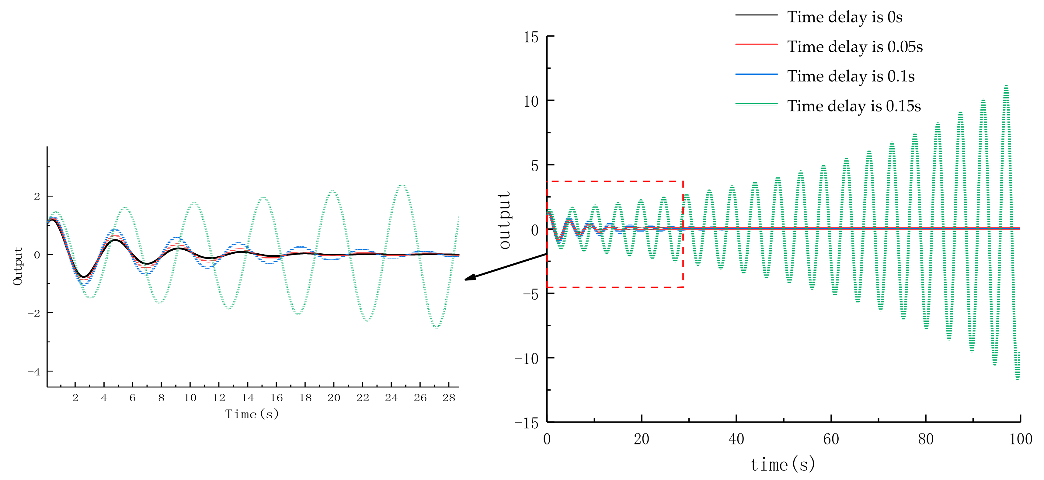
To illustrate the effect of time delay on the performance of the network control system, the output of the system with a sampling period of 0.1 s under the influence of different time delays is simulated and analyzed by using the above network control system model.
As seen in Figure 2, when the time delay is less than the system sampling period, the control performance of the system decreases significantly as the time delay increases. However, for a fixed time delay, the system can still achieve the expected output through its regulation as time passes. When the time delay is more significant than the system sampling period, it will cause the loss of system sampling information, and the system will lose stability as time goes on.

3. An Offline RBF Neural Network Delay Prediction Model Based on the Improved PSO Algorithm

3.1. Offline RBF Neural Network Prediction Model

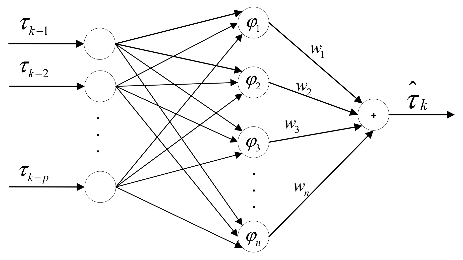
To predict the time delay of some sampling of the network control system, information from several delays must be known prior to the delay. Let the value of the delay of the kth sample to be forecast be τ k , the known τ k p as the input to the neural network, where p = 1, 2, ......, d, where d is the number of input nodes of the neural network. Once computed, the output τ ^ k value of the neural network is the expected delay of the kth sample.
The RBF neural network belongs to the three-layer forward neural network category, which has the characteristics of simple network structure, simple and fast network training, strong self-learning ability, strong nonlinear fitting ability, and fast convergence speed. It has the best approximation to global uniqueness. The delay prediction model of its composition is shown in Figure 3.
In order to facilitate the data processing and to speed up the convergence of the neural network, the input data are normalized to between −1 and 1, and the normalized mapping relations are as follows:
Y = 2 X X min X max X min 1
where X max and X min are the maximum and minimum values of the input data, respectively, and Y is the normalized output value. After the RBF neural network is computed, the output value must be inversely normalized to obtain the actual delay prediction value. The inverse function of Equation (12) is the inverse normalized mapping relation:
X = Y + 1 X max X min 2 + X min
A Gaussian kernel function is used as the nonlinear activation function for the hidden layer:
φ i = e x c i 2 2 σ i 2
where the Euclidean paradigm is the equation x c i 2 = x c i T x c i . Each hidden layer neural node contains two parameters: c i is the center of the ith hidden layer neural node and σ i 2 is the magnitude of the ith hidden layer neural node. x is the input vector, x = τ k 1 , τ k 2 , , τ k p T .
The output of the hidden layer neural nodes is multiplied by the weighting factor w n , which gives the predicted delay for the kth sample τ ^ k . The output of the delay prediction model can thus be expressed as:
τ ^ k = i = 1 n w i φ i = i = 1 n w i exp x c i 2 2 σ i 2

3.2. Particle Swarm Optimization Algorithm

The particle swarm algorithm has the advantages of fast convergence and simple operation. It is suitable for searching for the optimal solution in a dynamic multi-objective environment. It can converge quickly to the optimal solution with the highest probability, considering individualization and globalization. When a particle swarm finds a single pole p b e s t and the global extremum g b e s t , the particles update their velocity and position according to Equations (16) and (17):
v i j ( k + 1 ) = μ v i j ( k ) + c 1 r 1 [ p b e s t ( k ) x i j ( k ) ] + c 2 r 2 [ g b e s t ( k ) x i j ( k ) ]
x i j ( k + 1 ) = x i j ( k ) + v i j ( k + 1 )
where i = 1 , 2 , , M , j = 1 , 2 , , N , k and k + 1 are the number of previous iterations and the number of current iterations, respectively, v i j and x i j are the velocity and position of the particle, respectively, μ is the inertia weight, c 1 and c 2 are the learning factors, r 1 and r 2 are random numbers in the range [0, 1].
By adjusting the inertia weights, the local search ability and the global search ability of the algorithm are balanced. To address the problem that the commonly used linear decreasing strategy has a significant overhead and low search efficiency, and is prone to fall into local optimum at a later stage and cannot improve the solution of the algorithm, combined with the feature that the particle position gradually tends to be optimal as the degree of adaptation decreases, this paper proposes a nonlinear dynamic adjustment formula for the weights based on the degree of adaptation of the particles.
μ = μ min + ( μ max μ min ) 10 r a n d ( ) · ( ln f i ln f g b e s t ) 2 ( ln f ¯ ln f g b e s t ) 2
where μ min is the minimum value of the inertia weight, usually 0.4; μ max is the maximum value of the inertia weight, usually 0.9; r a n d ( ) is a random number from 0 to 1; f i is the fitness value of the ith particle at the current iteration number; f g b e s t is the optimal fitness value of the particle at the current population; f ¯ is the average fitness value of the particle at the current population.
In this paper, the weight of μ changes nonlinearly and dynamically with the difference between the fitness of the current particle and the optimal fitness of the population particles. When the difference is slight, the particle is within the optimal range, then the weight μ is small and the particle has strong local search ability; when the difference is significant, the particle is moving away from the optimal range, then the weight μ is large and the particle has strong global search ability. Particles are better at global searches. In addition, because the particles change with their own fitness, each particle has a different fitness, which improves the diversity of the particle population and increases the speed of the particle search. Combining the above characteristics, the nonlinear dynamic adjustment method of weights based on particle fitness proposed in this paper can improve the efficiency and accuracy of the PSO algorithm for finding the best weight.
In the PSO algorithm, the learning factor c 1 determines the individual’s “self-perception” and c 2 determines the individual’s “social perception.”. This paper uses an optimization strategy with asynchronous changes in learning factors in the optimization process of the two learning factors. This strategy allows the algorithm to learn more from the self-optimal and less from the group-optimal in the early stage of the optimization search to improve the global search ability of the particle swarm; and to learn more from the group-optimal and less from the self-optimal in the later stage of the optimization search, so that the particle swarm can converge to the optimal global solution quickly. The learning factor transformation formula used is shown in Equation (19).
c 1 = c 1 int ( c 1 int c 1 f i n ) t T c 2 = c 2 int + ( c 2 f i n c 2 int ) t T
where c 1 int and c 2 int are the initial values of the learning factors c 1 and c 2 , c 1 f i n and c 2 f i n are the final values of the iterations of the learning factors c 1 and c 2 , t is the current number of iterations and T is the maximum number of iterations.

3.3. PSO-RBF Time-Delay Prediction Model

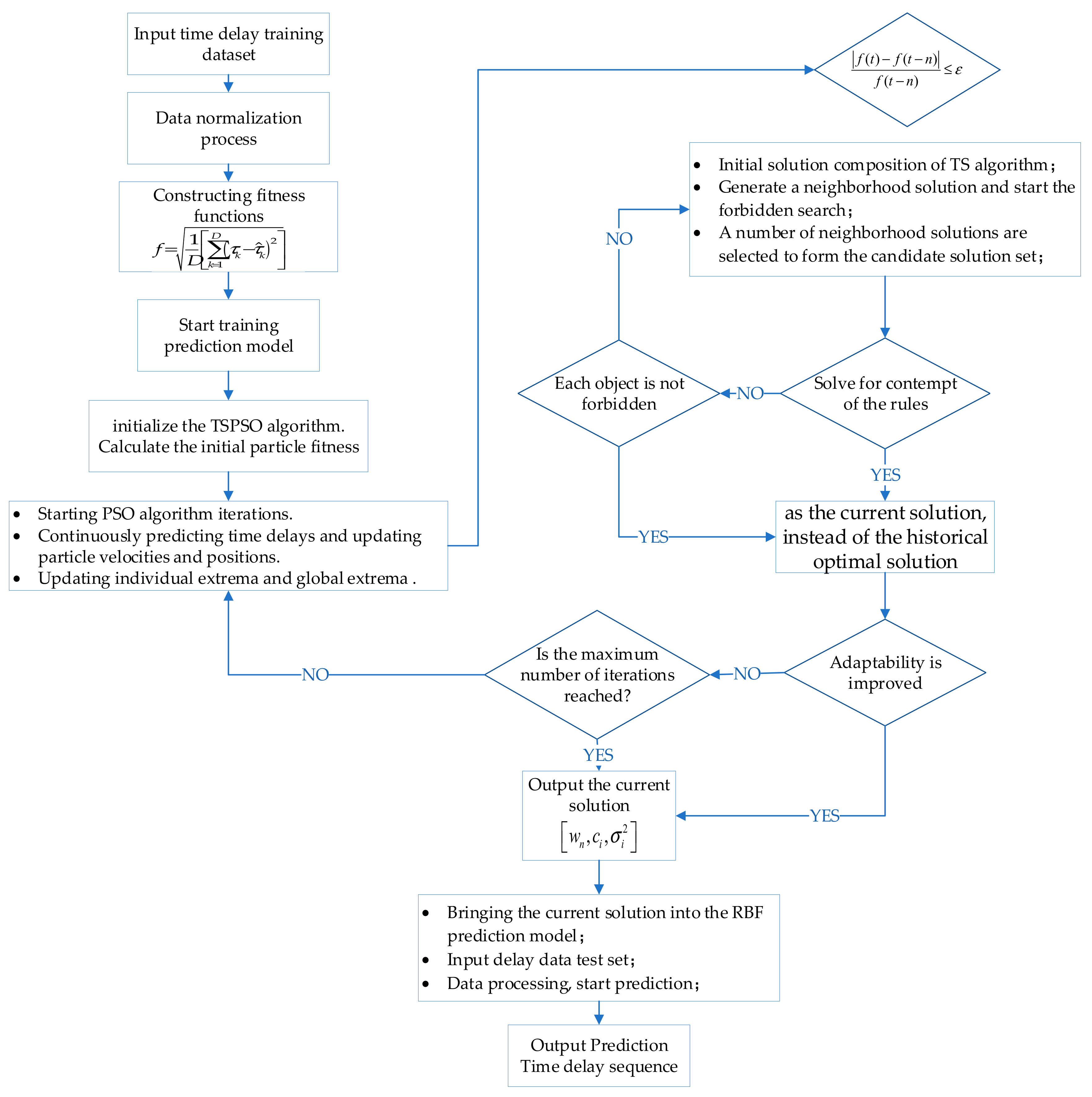
The parameters of the RBF neural network have a significant impact on the performance of the time-delay prediction model. In this artic, the PSO algorithm is used to optimize the three parameters of the RBF neural network: the amplitude of neural nodes in the RBF hidden layer σ i 2 , the center of neural nodes in the RBF hidden layer c i , and the connection weights w i . The specific steps of the PSO algorithm to optimize the delay prediction model are as follows:
Step 1: Normalize the input time-delay training set.
Step 2: Determine the number of neuron nodes n of the RBF neural network by means of a decremental clustering algorithm.
Step 3: Construct the fitness function. RBF neural networks usually use the root mean square error as the fitness evaluation function, as shown in Equation (20):
f = 1 D k = 1 D τ k τ ^ k 2
where D is the total number of predictions, τ k is the kth measured delay and τ ^ k is the kth predicted delay.
Step 4: Initialize each parameter of the particle swarm algorithm and the taboo search algorithm, calculate the initial fitness of the particles, and empty the taboo table.
Step 5: Continuously update the position and velocity of the particles by predicting the time delay from the model and update the individual extremes p b e s t and the global extremes g b e s t according to the fitness function.
Step 6: Determine whether the optimal solution of the particle swarm algorithm satisfies the taboo search start criterion, if not, go to step 5; otherwise proceed to the next step. The forbidden search start criterion is defined as:
f ( t ) f ( t n ) f ( t n ) ε
where f t is the fitness value for the current iteration, f ( t n ) is the fitness value before the n generation, and ε is the convergence threshold.
Step 7: The optimal solution generated by the particle swarm algorithm w n , c i , σ i 2 is binary encoded and combined into a three-dimensional binary encoded string, which forms the initial explanation for the forbidden search.
Step 8: Randomly generate several domain solutions based on the current solution, perform a forbidden search, and select the best-adapted domain solutions from them.
Step 9: Determine whether there is a contempt criterion-compliant solution in the candidate solution set; if so, consider the most optimal solution that meets contempt criterion criteria as the current solution and replace the earliest taboo object on the taboo list with the corresponding forbidden thing, and replace the most optimal historical solution with that solution and move on to step 11; otherwise, proceed to the next step.
Step 10: Determine the taboo properties of each object corresponding to the candidate solution, select the optimal state corresponding to the non-taboo thing set in the candidate solution as the current solution, and replace the taboo item entering the taboo table for the first time with its corresponding forbidden object.
Step 11: Determine if the adaptation has improved and, if so, end the algorithm and output the current solution. Otherwise, continue to the next step.
Step 12: Determine whether the maximum number of iterations has been reached and, if so, terminates the algorithm and output the current solution. Otherwise, proceed to the next iteration.
The flow of the delay prediction model algorithm based on an improved offline PSO-RBF network is shown in Figure 4.

4. Online RBF Model Predictive Controller Design

4.1. Online RBF Network Single-Step Predictive Controller Design

RBF neural networks are characterized by high real-time performance and high nonlinear fit and have great promise for use in network control systems with time delays. Online RBF neural networks have the following characteristics compared to offline RBF neural networks.
  • The online RBF neural network is trained one by one with unknown maximum, minimum, and mean values, which cannot be normalized.
  • Online RBF neural networks are trained data-by-data and cannot be corrected using the global error guidance function for weights and thresholds. However, thanks to this feature, the online RBF neural network is somewhat resistant to interference when applied to the controller design.
  • The nodes of the hidden layer cannot be found using the K-means algorithm because the data set is not available in advance for online RBF neural networks.
In the design of the controller for the network control system, the computational volume of the controller should be reduced as much as possible in order for the controller to meet the demand of the system in real-time. At the same time, allowing the RBF neural network to fall into local optimal solutions should be avoided to ensure the control system’s performance. Based on the above two considerations, a single-step predictive controller based on an online RBF neural network is designed in this paper, formulated as follows:
u ( k ) = f N N C r ( k ) ; y ( k 1 ) ; u ( k 1 )
where u ( k ) is the control quantity at the current moment; u ( k 1 ) is the control quantity at the previous moment; f N N C is the online RBF neural network model; r ( k ) is the reference input at the current moment; and y ( k 1 ) is the actual output of the controlled object at the previous moment. Because the online RBF neural network cannot obtain the data set in advance, the number of nodes in the hidden layer is taken to be equal to the number of nodes in the input layer.

4.2. Rolling Optimization and Feedback Correction

An online RBF neural network predictive controller is designed in this paper, which adopts the idea of an optimal control algorithm. The core of this is online rolling optimization. Although the rolling optimization does not carry on the global whole optimization, but maintains the control principle, it carries on the gradual optimization over time, takes a target function based on, and only relating to, the system parameters at each moment, and carries on the system’s repeated online optimization.
Based on the traditional rolling optimization performance index, combined with the differential role in PID control, this paper proposes a new objective function:
J = [ u s ( k ) u ( k ) ] 2 + λ [ r ( k ) y ( k 1 ) ] 2 + [ e ( k ) e ( k 1 ) ] 2 e ( k ) = u s ( k ) u ( k ) e ( k 1 ) = u s ( k 1 ) u ( k 1 )
where u s ( k ) is the actual value of the control volume at the current moment, u s ( k 1 ) is the actual value of the control volume at the previous moment, λ is the optimization weight coefficient, the initial value of λ is a random number in the range of [−1,1]. Finally, [ e ( k ) e ( k 1 ) ] 2 is the differential, which reduces the overshoot of the system and shortens the adjustment time.
For the adjustment of the parameters of the online RBF neural network, this paper uses the gradient descent method to solve this optimization problem, and the adjustment formula for each coefficient is as follows:
w i ( k ) = w i ( k 1 ) + η [ u s ( k ) u ( k ) ] G i + α [ w i ( k 1 ) w i ( k 2 ) ] Δ σ i ( k ) = [ u s ( k ) u ( k ) ] w i G i O ( k ) c i ( k ) 2 σ i 3 σ i ( k ) = σ i ( k 1 ) + η Δ σ i ( k ) + α [ σ i ( k 1 ) σ i ( k 2 ) ] Δ c i ( k ) = [ u s ( k ) u ( k ) ] w i G i O ( k ) c i ( k ) σ i 2 c i ( k ) = c i ( k 1 ) + η Δ c i ( k ) + α [ c i ( k 1 ) c i ( k 2 ) ]
where η is the learning rate; α is the momentum factor, η 0 , 1 , α 0 , 0.1 ; and G is the Gaussian kernel function.
η and α are mainly used to rectify the three parameters of the online RBF predictive controller. η is mainly used to compensate the errors caused by the calculation, and its value should not be too large, and is usually taken in the range of [0, 1]. When α is invariant, the effect of η on the control quantity is shown in Figure 5. As can be seen from Figure 5, only when a is taken in the range of [0, 1], can the controller steadily provide the control amount to the control system; too large a value will lead to the controller overshoot phenomenon, and ultimately affect the stability of the system. The role of α is to regulate the three controller parameters of the adjustment process. The value should not be too large, generally in the range of [0, 0.1], because when its value is too large it will also cause the controller stability to decline, and cannot provide the system with a stable amount of control.
Feedback adjustment: due to the presence of influencing factors such as model mismatch or system disturbance, there is a specific error between the output of the predictive controller and the actual output. To reduce this error, feedback compensation can be made using the reference input and the predicted output, calculated as follows:
e m ( k + 1 ) = r ( k + 1 ) y m ( k + 1 ) + ζ e ( k )
where: e m ( k + 1 ) is the prediction error; r ( k + 1 ) is the reference input; y m ( k + 1 ) is the prediction output; ξ is the compensation factor, and e ( k ) is the current error.

5. Networked Control Systems Based on RBF Neural Networks

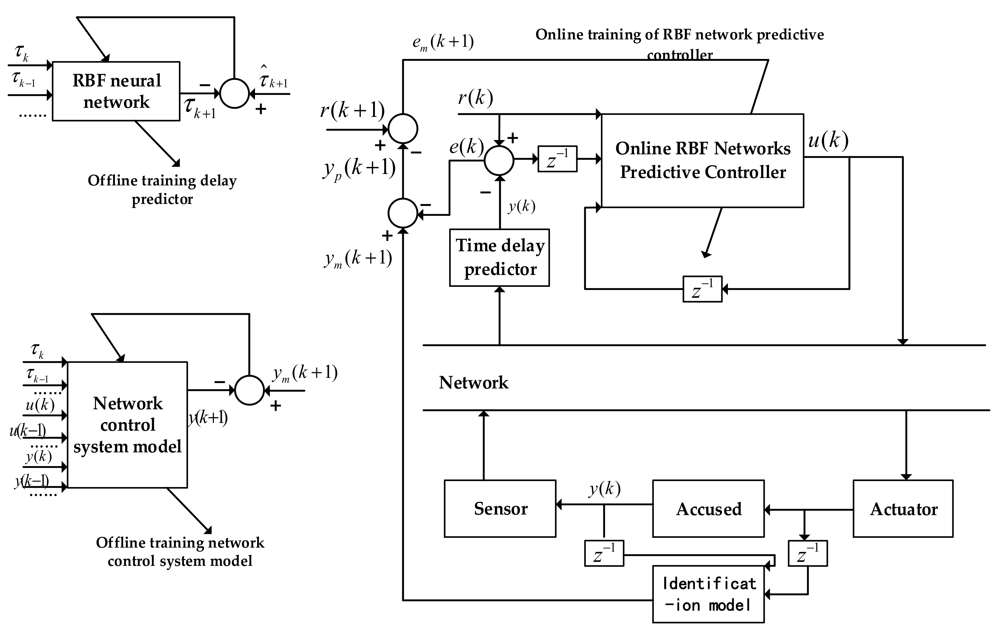
The overall system structure is shown in Figure 6. In the figure, τ indicates the predicted time delay; τ k indicates the measured value of the time delay; e indicates the error; u indicates the control quantity of the controlled object; y indicates the system output; r indicates the reference input of the system; and k 1 , k and k + 1 indicate the last sample time, the current sample time and the next sample time, respectively.
The design objectives and design parameters of the networked control system designed in this paper are as follows:
  • Design goal: the system is a networked control system with stochastic time-delay prediction and compensation, for situations where the time-delay model is known or unknown.
  • Controlled objects: for nonlinear control objects.
  • Delay models: for random delays, fixed delays and random delays that satisfy the Markov chain model.
  • System structure: straightforward structure.
  • Stochastic delay prediction model: an offline RBF network delay prediction model based on an improved PSO algorithm, i.e., the content in Section 3 of this paper.
  • Controller: online RBF neural network single-step predictive controller, i.e., what is in Section 4 of this paper.
  • Identification model: a network control system based on stochastic time delays, i.e., the contents of Section 2 of this paper.
  • System nodes are driven: the controller nodes and actuator nodes are event-driven, and sensor nodes are clock-driven.
  • Sampling period: The sampling period h is greater than the network transmission delay at any given moment τ k .
The overall operational flow of the system is as follows:
  • Sampling of data for offline training of RBF neural networks. The training data for the time-delay prediction model is the actual measurement data of the time delay, sampled and used to train the time-delay prediction; the input and output of the controlled object are collected and used to train the recognition model.
  • Determining the number of input nodes and the number of nodes in the hidden layer for the RBF neural network. The number of input nodes and the number of nodes in the hidden layer of the time-delay prediction model and online RBF network controller are problem-specific and need to be tested for errors to determine the number of nodes for said problem. Typically, satisfying the equation
    τ k + τ B < k h
  • where: τ k is the overall system time delay; τ B is the time-delay difference generated by the system after time-delay compensation; k is the number of steps; and h is the sampling frequency.
  • In the case that the sampling frequency is set appropriately, and the delay can be accurately predicted in most cases, single-step predictive control is used, and k is taken as 1.
  • Initialization of the delay prediction model, the controller, and the recognition model.
  • Controller response. The amount of control u ( k ) at the current moment of the controlled object is calculated by r ( k ) , y ( k 1 ) , and u ( k 1 ) ; the time-delay prediction is performed by a time-delay prediction model with the completion of offline training, and the time delay is compensated.
  • After predicting and compensating for time delay, actuator response, controlled object response, sensor response, and sample completion, the system returns to step (4).

6. System Simulation and Analysis of Results

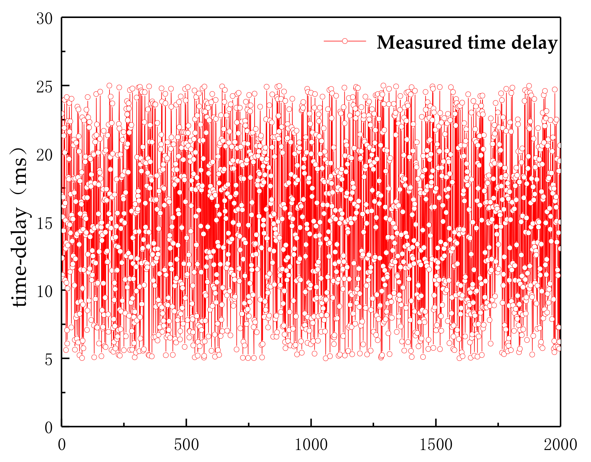
The time-delay sequences used to train the offline RBF neural network time-delay prediction model in this paper come from 2000 sets of measured data collected using an Intel I5 processor-based host computer communicating with an IMX6ull-based motion control board, with a sampling interval of 100 ms and the equipment running continuously for 200 s. The sampled delay sequence is shown in Figure 7. The first 1500 sets of data were selected as the training set and the last 500 sets of data were used as the test set to build an offline delay prediction model for the improved PSO-RBF network, and the prediction model was updated during the control process. Afterward, the accuracy of the predictive control method proposed in the paper is verified on the network control system model established in this paper for the delay prediction model of the network control system with random delays, and the system performance of the controller based on the compensation of random delays.

6.1. Validation of the Offline Delay Prediction Model

In order to verify the superiority of the adaptation-based nonlinear weight adjustment formula proposed in this paper for the PSO algorithm in the optimization search process, a comparative simulation of the PSO algorithm for superiority seeking under four different weight adjustment formulas is performed by using the same learning factor adjustment formula, as shown in Figure 8.
As can be seen from Figure 8, in terms of the speed of finding the optimal solution, the weight adjustment formula proposed in this paper has arrived near the optimal solution at the sixth iteration compared with the other weight adjustment formulas, indicating that the nonlinear dynamic adjustment formula based on the degree of adaptation proposed in this paper has a more assertive global search ability and faster speed of finding the optimal solution. In terms of optimization-seeking accuracy, the nonlinear adjustment formula and the adaptive adjustment formula are better than the other two adjustment formulas. It can be seen from the curves that the nonlinear adjustment formula can quickly jump out of the local optimum after finding the local optimum solution, which meets the requirements of the network control system designed in this article.
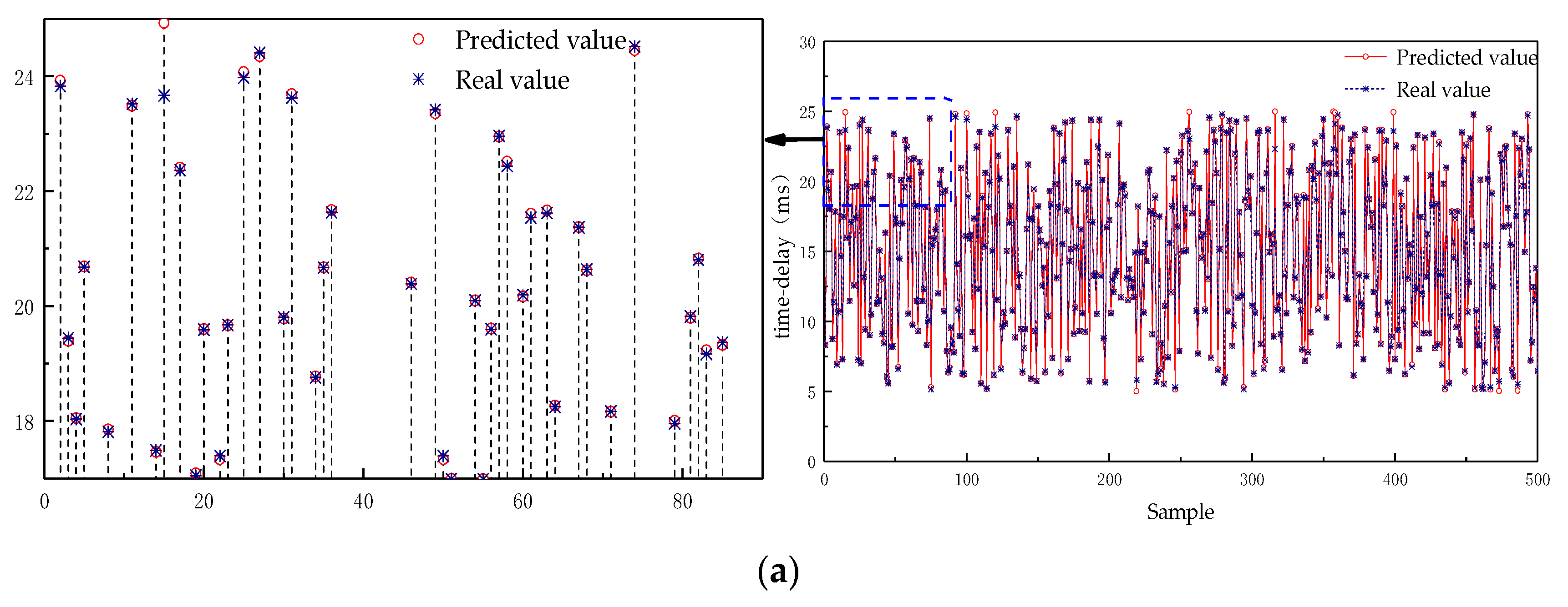
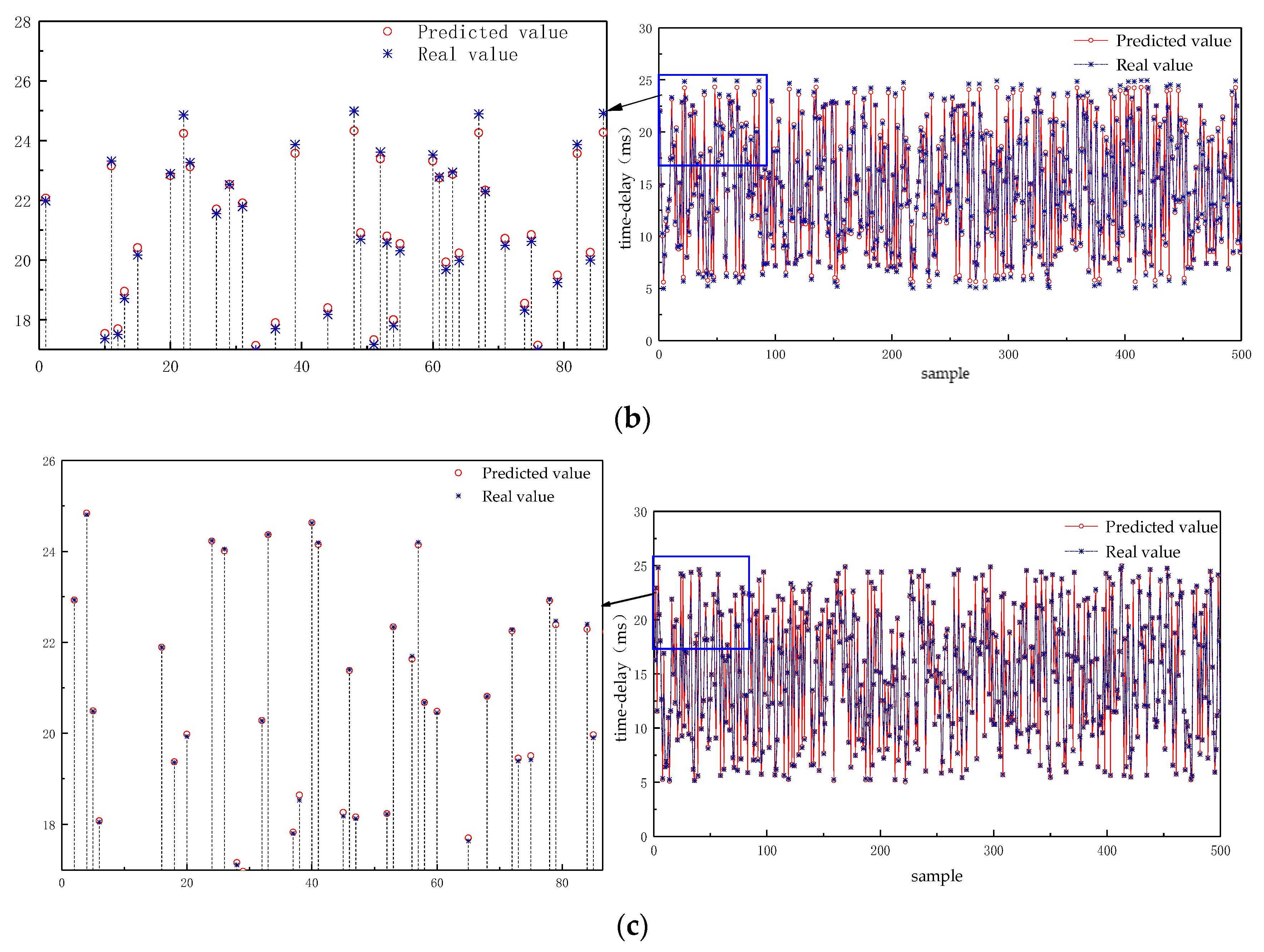
In order to verify the prediction performance of the improved PSO-RBF network offline delay prediction model, three algorithms are used to predict the measured delay. The minimum inertia weight of the PSO algorithm μ min = 0.4, the maximum inertia weight μ max = 0.9, the initial values of c 1 and c 2 are 2 and 0.5, respectively, the maximum number of iterations is 500, the convergence threshold is 0.001, and the number of nodes in the hidden layer of the RBF neural network is confirmed to be five by the K-means algorithm. All three algorithms have a 10-input-1-output structure, and the test set is processed in a chaotic order. A comparison of the predictions of the three different prediction methods is shown in Figure 9.
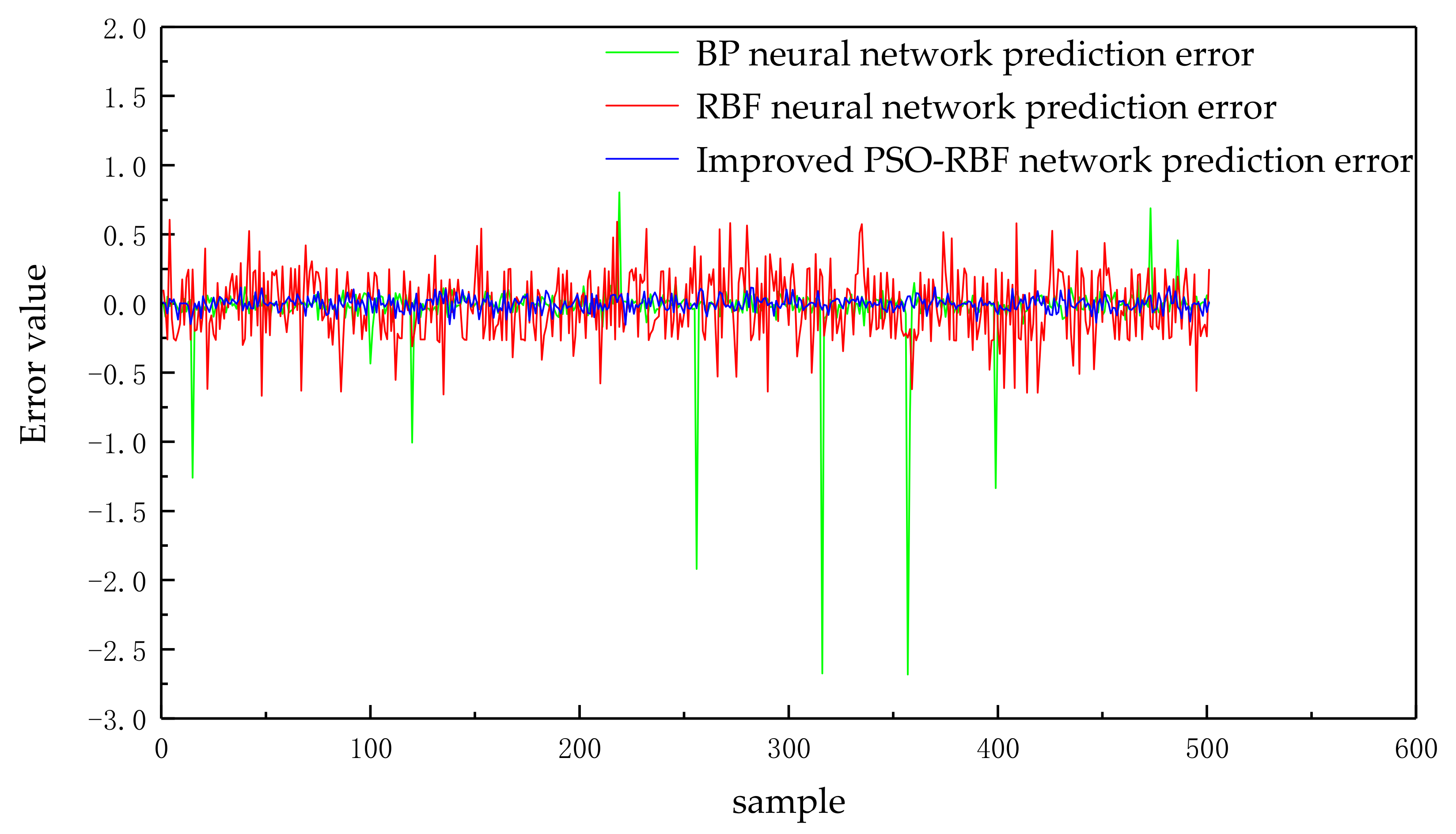
From the comparative analysis in Figure 9, it can be seen that the predicted values obtained by the improved PSO-RBF prediction algorithm fit the real values better than both the BP neural network and the original RBF neural network, and the original RBF neural network performs the worst fit among the three. In the peak and trough regions, the predicted values obtained by the RBF neural network differed significantly from the actual values and were barely fitted. The BP neural network’s predictions in the peak region were also not respectable. Figure 10 shows a comparison of the error curves for each prediction algorithm. From Figure 10, it can be more intuitively seen that the improved PSO-RBF neural network offline delay prediction control system proposed in this paper has the most minor error between the predicted and actual values, and the error is relatively stable without substantial changes, while the RBF neural network has more significant fluctuations in the error of each prediction compared to the previous one, and the error curve is relatively complex and cannot accurately predict the delay. The neural network in the prediction process appears to have significant error fluctuations, is not conducive to the system’s stability, and cannot meet the needs of the network control system.
To further validate the superiority and effectiveness of the PSO-RBF neural network offline delay prediction model in predicting stochastic delays, root mean square error (RMSE), mean absolute error (MAE), and cycle prediction time were used to evaluate the performance of the prediction algorithms. Table 1 presents the average prediction performance of different prediction algorithms for 10 independent predictions.
M A E = 1 Q t = 1 Q τ t τ ^ t R M S E = 1 Q t = 1 Q ( τ t τ ^ t ) 2
where τ t is the delay observation; τ ^ t is the delay prediction; and Q is the sample size.
As can be seen from Table 1, the RMSE, MAE and cycle prediction times for the improved PSO-RBF network prediction delay are 0.0105, 0.0383, and 1.38, respectively, which are 56.6%, 44.3%, and 71.3% lower compared to the BP neural network, and 21.7% and 81.2% lower compared to the RBF neural network, respectively, indicating the PSO-RBF neural network’s prediction performance compared to the other two algorithms. The deviation between the predicted and true values of the PSO-RBF neural network is much smaller than that of the different algorithms, which indicates that the offline delay prediction model of the PSO-RBF network proposed in this paper has excellent prediction performance and the fit between the predicted and actual values is high. This is because, compared with the RBF neural network, the PSO algorithm reduces the uncertainty caused by the random parameters of the RBF neural network in the prediction model designed in this paper, and improves the prediction accuracy of the RBF neural network. The prediction time of the PSO-RBF neural network prediction model is more significant than that of the RBF neural network due to the addition of the RBF parameter-adaptive optimization-seeking algorithm. However, it is still smaller than the sampling cycle time when added to the measured value of the time delay, which has less impact on the system performance and meets the demand of the system predictor in real time.

6.2. Control Performance Analysis of Network Control Systems Based on Rbf Neural Networks

This paper uses MATLAB’s network control system simulation platform True-Time to simulate and verify the control performance of a network control system based on RBF neural networks. The following servo control system is considered to be built, with the transfer function of the controlled object:
G ( s ) = 1000 s ( s + 25 )
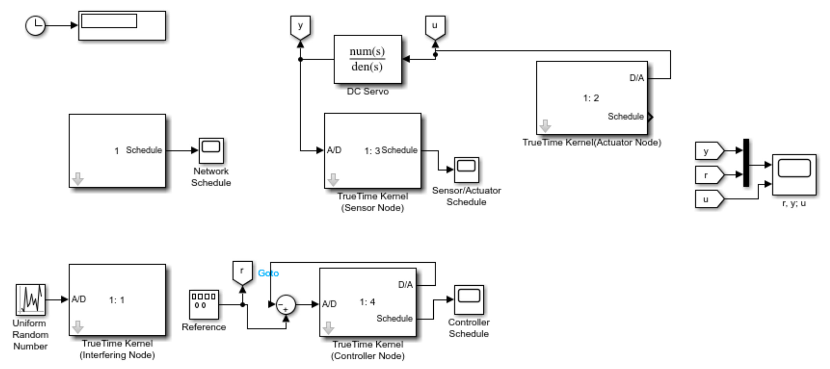
In the networked control system model, the system sampling period is set to T = 10   m s , the network transmission method is selected as the Ethernet communication protocol, the order of information transmission is determined according to priority, the data transmission rate is set to 100,000 b i t s / s , and the minimum frame size is 80 b i t s ; the packet size is 80 b i t s . The RBF neural-network-based networked control system built using the True-Time 2.0 toolbox is shown in Figure 11. The three kernel modules in the toolbox are used to simulate the corresponding jamming node, controller, and sensor/actuator in the system. The network uses the network module from the True-Time toolbox. The prediction model was set with a minimum PSO algorithm inertia weight of μ min = 0.4, a maximum inertia weight of μ max = 0.9, initial values of 2 and 0.5 for c 1 and c 2 , respectively, a maximum number of iterations of 500, and a convergence threshold of 0.001. The number of input nodes for the offline PSO-RBF neural network delay prediction model is 10, the number of nodes in the hidden layer is confirmed to be 5 by the K-means algorithm several times, and the number of nodes in the output layer is 1. The number of nodes in the input layer and the number of nodes in the hidden layer of the online RBF neural network predictive controller is both 3, the number of nodes in the output layer is 1, the gradient descent learning rate η was set to 0.3, and the momentum factor α was set to 0.01.
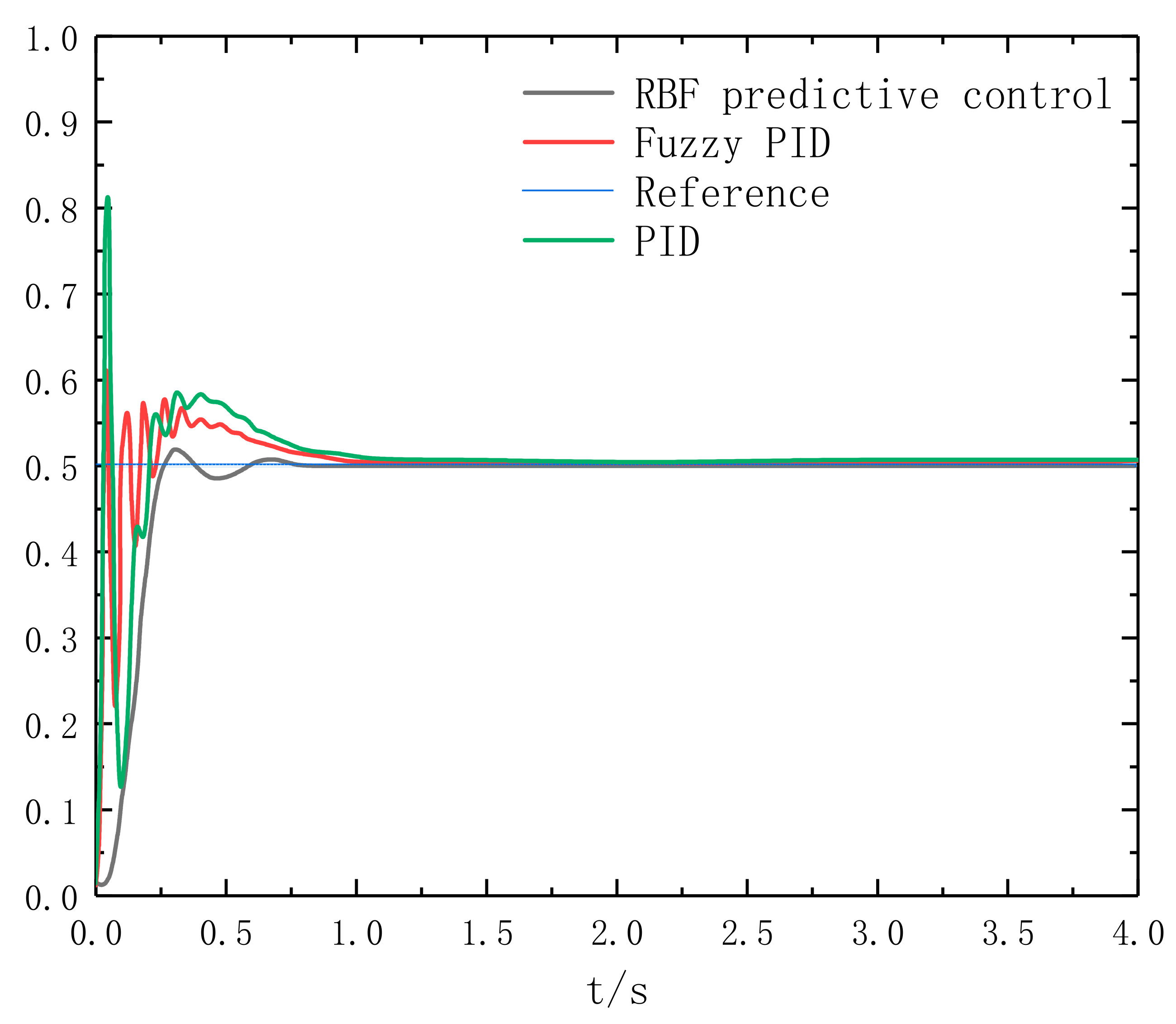
In order to verify the method of this paper, the predictive control model proposed in this paper was compared and analyzed with the PID control algorithm, where the input signal is a square wave signal, and the simulation results are shown in Figure 12.
In Figure 12, online RBF predictive control is compared with traditional PID control for a network control system with random time delay. The networked control system proposed in this paper can give more accurate control output in a more timely manner, so that the system output can track the reference trajectory of the output of the second-order control object faster, and the overshoot and adjustment time are better than the PID control algorithm to meet the performance requirements of the system. Although all three control methods can achieve the desired control effect after a period of adjustment, in terms of time, RBF predictive control achieves the desired control effect faster than fuzzy PID control, and the tracking speed during the rise and fall process is also faster to meet the demand of system in real time. In contrast, fuzzy PID control and PID control show a certain amount of overshoot after the rising and falling stages. The reason for this may be that the PID algorithm needs some time to learn to make the control effect stable after the change of reference signal.
In order to further verify the control effect of the control system designed in this paper, the control effect is evaluated by using the integral of absolute error (IAE), in integral time absolute error (ITAE) with the following formula.
I A E = 1 K t = 1 K r ( t ) y ( t )
I T A E = 1 K t = 1 K t r ( t ) y ( t )
where k is the total number of samples and r ( t ) , y ( t ) is the reference input and control output at time t, respectively.
Table 2 shows the comparison of the evaluation indices of different controllers for networked control with random time delays. It can be seen that the performance of I A E and I T A E is 0.0831 and 0.0734, respectively, which is 68.2% and 70.2% higher than that of PID controller, and 30.5% and 31.3% higher than that of fuzzy PID control. The results show that the proposed RBF neural-network-model-based predictive control system has better adaptive and disturbance suppression capabilities in networked control systems with random time delays, and can achieve more accurate compensation for random time delays.
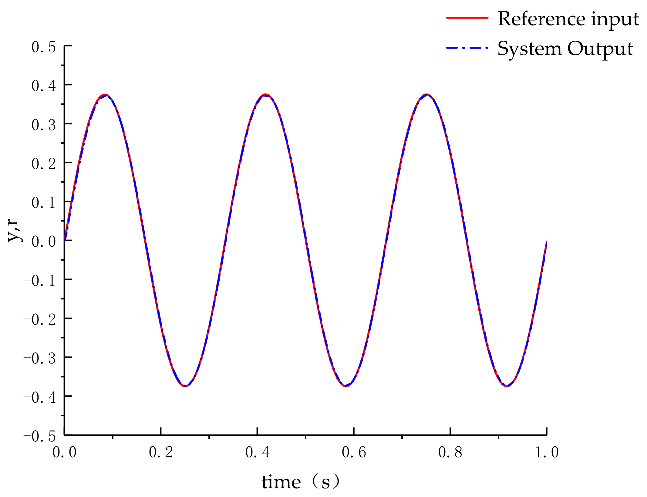
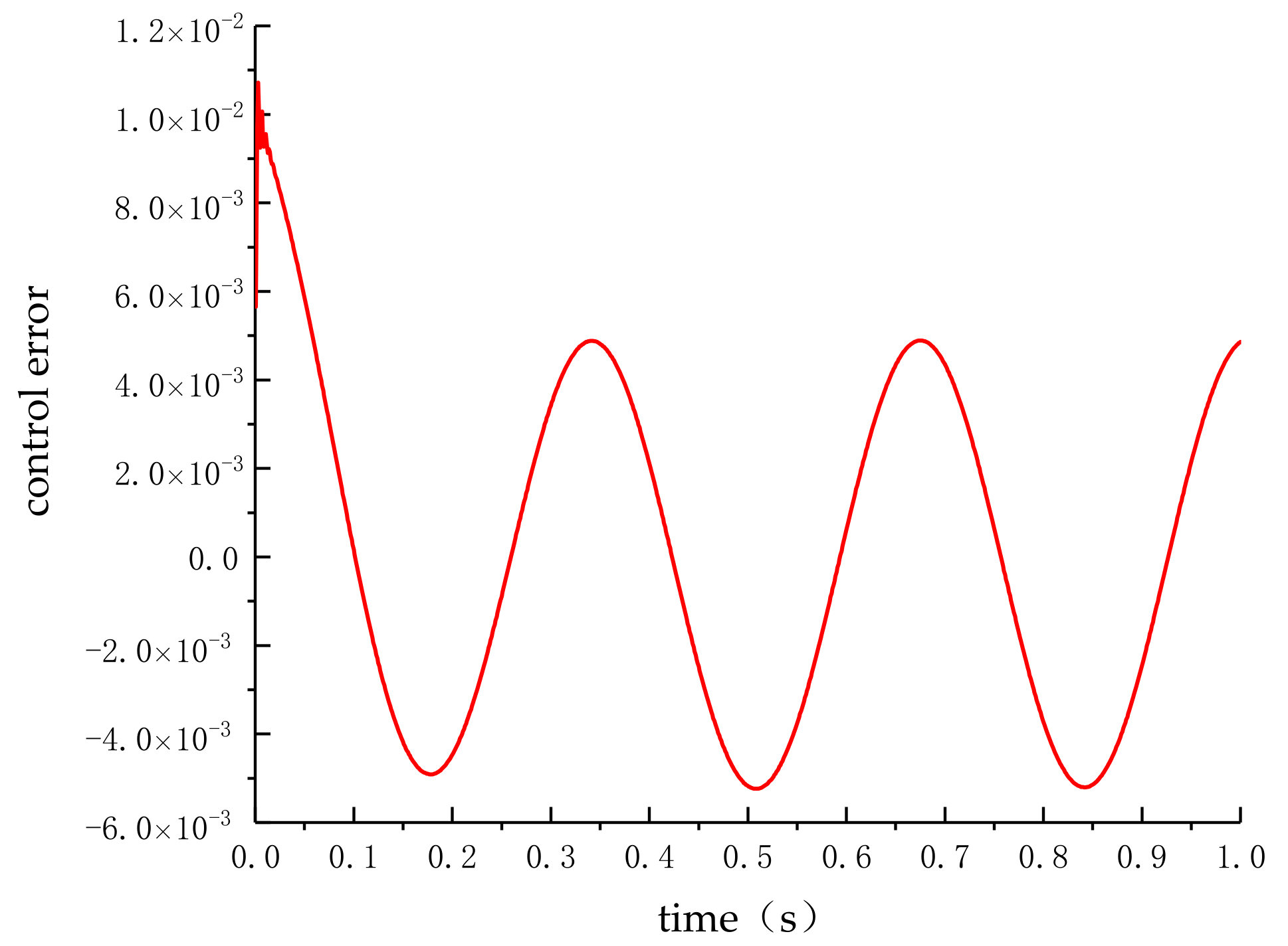
When the input signal is a sine wave signal, the system control effect and control error is shown in Figure 13 and Figure 14. From Figure 13, it can be seen that the output of the network control system designed in this paper can follow the sine wave signal well, and the fit with the reference value is high, which can meet the demand of the system control performance. Analyzing the error curve in Figure 14, it can be seen that the prediction error of the network control system designed in this paper is more significant at the beginning of the control phase and there is jitter. This is because the online RBF network predictive controller needs a certain amount of time for training to perform effective control, and the jitter time is shorter, indicating that the online RBF predictive control model has a better learning ability and tracks the sine wave signal better than the opposing wave signal.
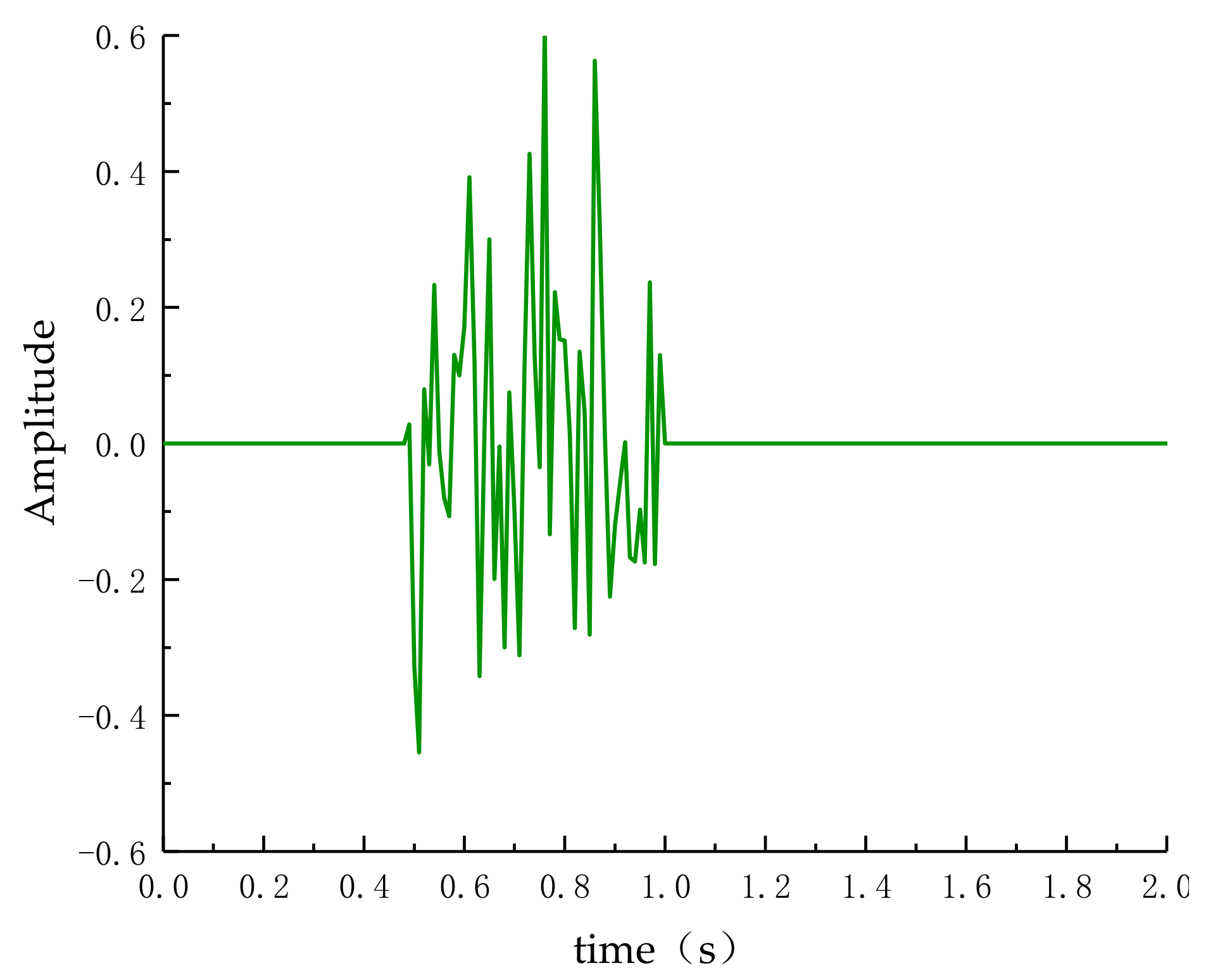
As network control has uncertainty disturbance in the actual control process, this paper simulates this situation by adding Gaussian white noise in the form of a time period of 0.5   s < t < 1   s ; the waveform of Gaussian white noise is shown in Figure 15.
Under the influence of the disturbance signal, the control effect of the network control system and the PID control algorithm proposed in this paper is compared as shown in Figure 16. As can be seen from the control curve in Figure 16 after 1 s, the PID algorithm needs to readjust the control parameters after the disturbance signal is added and overshoot occurs after 1.5 s; the control effect on the controlled object is not ideal and cannot meet the control requirements of the system. The control algorithm proposed in this paper has specific anti-interference ability and can quickly re-tune the model to provide accurate control output after disturbance signal so that the system can track the reference input trajectory faster and meet the demand of the control system.
To further verify the control effect of the control system designed in this paper under the action of a disturbance signal, the two indicators of IAE and ITAE mentioned previously in this article are used to evaluate the performance of different controllers under the influence of disturbance signals for networked control with random time delay, and the comparison of the evaluation results is shown in Table 3. It can be seen that the IAE and ITAE of RBF predictive control are 0.1248 and 0.1196, respectively, which are 59.9% and 67% improved compared to the PID controller, and 31.7% and 27.8% improved compared to the fuzzy PID control, respectively. The results show that under the influence of disturbance signals, the proposed RBF neural-network-based predictive control system has better adaptive and disturbance suppression ability and can achieve more accurate compensation for the random time delay.

6.3. Physical Verification of Network Control System Based on RBF Neural Network

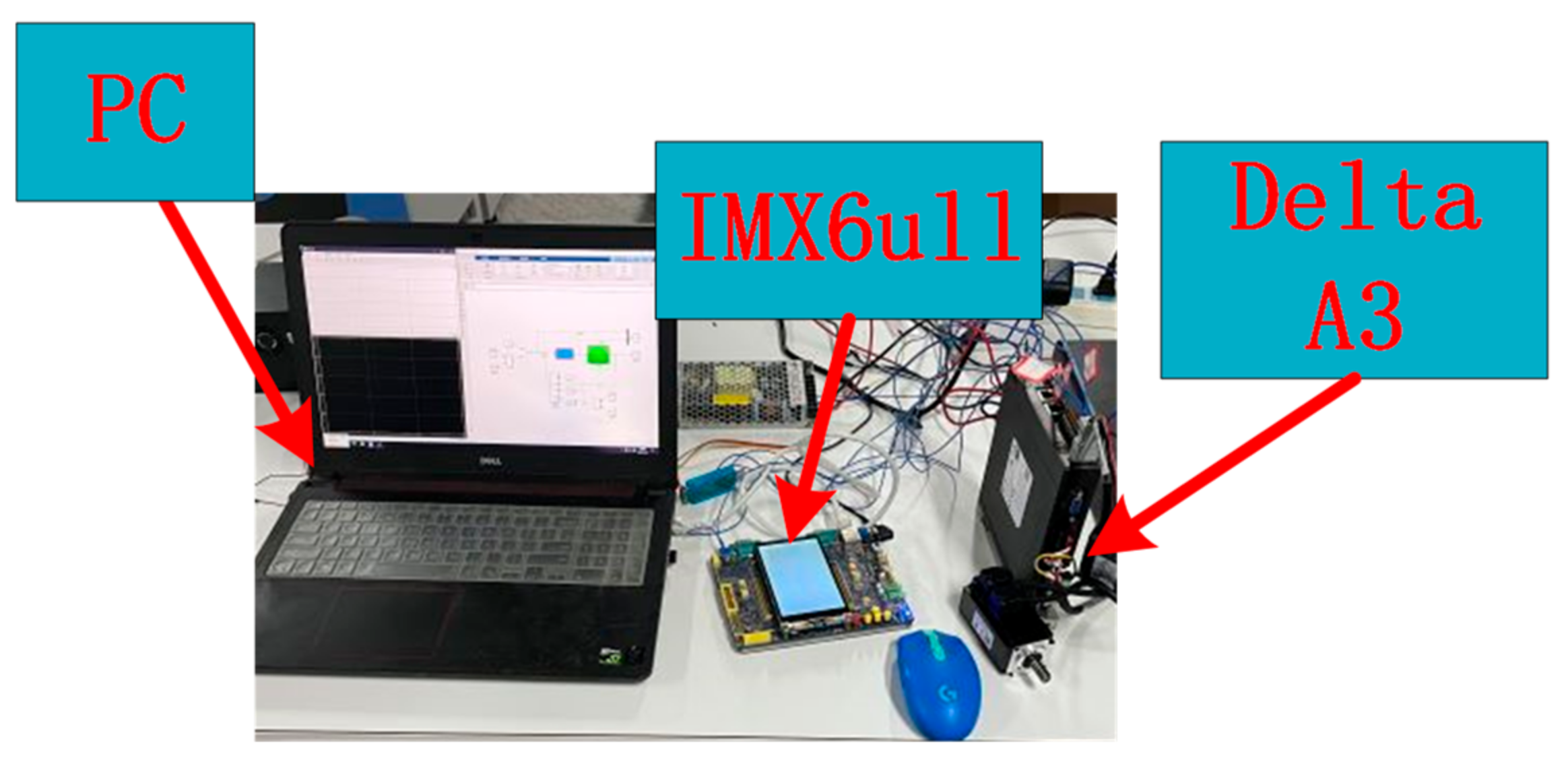
In order to verify the practicality and effectiveness of the method proposed in this paper, a physical platform was built as shown in Figure 17, which consisted of a PC, a motion controller, a servo controller and a servo motor. The PC was used as the upper computer, which integrates the controller and time-delay prediction. The actuator was a Linux motion control board with IMX6ull as the kernel and burned with a discriminative model program. A Delta A3 series servo controller and servo motor were used as the controlled objects, and the motor output was monitored by the servo controller to play the role of a sensor. In this system, the PC communicates with the motion control board and the servo system via Ethernet, and the motion controller communicates with the servo system via a serial port.
In order to demonstrate the effectiveness and practicality of the network control system based on PSO-RBF delay prediction model proposed in this paper, three methods, namely, traditional PID control, fuzzy PID control and the control algorithm proposed in this paper, were compared experimentally. The parameters of the network control system based on the PSO-RBF experimental prediction model were set in accordance with Section 6.2. The experimental results are shown in Figure 18. The algorithm proposed in this paper outperforms the other two algorithms in terms of overshoot and regulation time. From Figure 18, it can be seen that the system output of the algorithm proposed in this paper is slower than the other two algorithms in the first 0.5 s of regulation, which is because the online RBF prediction controller needs some time to learn for effective control, and the experimental results show that the network control system based on the PSO-RBF delay prediction model has a better ability to predict and compensate for the delay than the traditional algorithm

7. Conclusions

To address the impact of random time delay on system performance in network control systems, based on the requirements of real-time and accurate control systems, this paper proposes a predictive control system based on the PSO-RBF network model. Firstly, a network control system model with stochastic time delay is established, and its discrete state equations are obtained for the identification system of the network control system. Secondly, for the problem of time-delay prediction, this paper proposes an offline predictive controller based on an improved PSO-RBF network, adopts the PSO algorithm for adaptive control of the parameters of the RBF neural network, proposes a new way of adjusting the parameters of the PSO algorithm to address the problem that the PSO algorithm tends to fall into local optimality in the late iteration. The late iteration of the PSO algorithm is improved by using the banned search algorithm. The simulation proves that the offline prediction controller based on the improved PSO-RBF network proposed in this paper reduces RMSE, MAE and Cycle Forecast Time by 56.6%, 44.3%, and 71.3%, respectively, compared with BP neural network, and RMSE and MAE by 21.7% and 81.2%, respectively, compared with RBF neural network, and can make an accurate prediction of time delay and has a shorter prediction period to meet the real-time system requirements. To address the impact of time delay on the control performance of the network control system, an online RBF network predictive controller is designed to compensate for the time delay, and the parameters of the online RBF network are adjusted using the gradient descent method. In order to improve the performance of the predictive controller, an objective function is proposed in the rolling optimization stage to evaluate the optimization effect. Experimental results demonstrate that the predictive controller for online RBF networks proposed in this paper has reasonable control over both the compensation problem of time delay and the output of the system under the influence of uncertainty disturbances. However, the method proposed in this paper still has some limitations. The nodes of the hidden layer of the RBF neural network used in this paper and the values of some parameters need to be confirmed by a large number of experiments. The application of this predictive control system in networked multi-axis control systems will be further investigated later.

Author Contributions

Y.L. wrote the manuscript and designed the research methodology; D.Y. edited and revised the manuscript; S.L. and M.Z. collected the data; Y.Z. processed the data. All authors have read and agreed to the published version of the manuscript.

Funding

This work was supported by the National Natural Science Foundation of China (Grant Number 51875180).

Institutional Review Board Statement

Not applicable.

Informed Consent Statement

Not applicable.

Data Availability Statement

Data are contained within the article. The data presented in this study can be requested from the authors.

Conflicts of Interest

The authors declare no conflict of interest.

References

  1. Mahmoud, M.S.; Sabih, M. Experimental Investigations for Distributed Networked Control Systems. IEEE Syst. J. 2014, 8, 717–725. [Google Scholar] [CrossRef]
  2. Ding, L.; Han, Q.-L.; Wang, L.Y.; Sindi, E. Distributed Cooperative Optimal Control of DC Microgrids With Communication Delays. IEEE Trans. Ind. Inform. 2018, 14, 3924–3935. [Google Scholar] [CrossRef]
  3. Sandberg, H.; Amin, S.; Johansson, K. Cyberphysical Security in Networked Control Systems: An Introduction to the Issue. IEEE Control Syst. 2015, 35, 20–23. [Google Scholar] [CrossRef]
  4. Wang, Y.-L.; Han, Q.-L. Network-Based Modelling and Dynamic Output Feedback Control for Unmanned Marine Vehicles in Network Environments. Automatica 2018, 91, 43–53. [Google Scholar] [CrossRef]
  5. Zhang, X.-M.; Han, Q.-L. Network-Based H-Infinity Filtering Using a Logic Jumping-like Trigger. Automatica 2013, 49, 1428–1435. [Google Scholar] [CrossRef]
  6. Zhang, X.-M.; Han, Q.-L.; Ge, X.; Ding, D.; Ding, L.; Yue, D.; Peng, C. Networked Control Systems: A Survey of Trends and Techniques. IEEE/CAA J. Autom. Sin. 2020, 7, 1–17. [Google Scholar] [CrossRef]
  7. Hu, Z.; Deng, F.; Xing, M.; Li, J. Modeling and Control of Itô Stochastic Networked Control Systems With Random Packet Dropouts Subject to Time-Varying Sampling. IEEE Trans. Automat. Contr. 2017, 62, 4194–4201. [Google Scholar] [CrossRef]
  8. Zhiwen, W.; Ge, G. Fundamental Issues and Prospective Directions in Networked Multirate Control Systems. Math. Probl. Eng. 2014, 2014, 1–10. [Google Scholar] [CrossRef] [Green Version]
  9. Qiu, J.; Gao, H.; Ding, S.X. Recent Advances on Fuzzy-Model-Based Nonlinear Networked Control Systems: A Survey. IEEE Trans. Ind. Electron. 2016, 63, 1207–1217. [Google Scholar] [CrossRef]
  10. Ge, X.; Yang, F.; Han, Q.-L. Distributed Networked Control Systems: A Brief Overview. Inf. Sci. 2017, 380, 117–131. [Google Scholar] [CrossRef]
  11. Yuan, H.; Bi, J.; Tan, W.; Zhou, M.; Li, B.H.; Li, J. TTSA: An Effective Scheduling Approach for Delay Bounded Tasks in Hybrid Clouds. IEEE Trans. Cybern. 2017, 47, 3658–3668. [Google Scholar] [CrossRef] [PubMed]
  12. Yuan, H.; Bi, J.; Tan, W.; Li, B.H. Temporal Task Scheduling With Constrained Service Delay for Profit Maximization in Hybrid Clouds. IEEE Trans. Autom. Sci. Eng. 2017, 14, 337–348. [Google Scholar] [CrossRef]
  13. Bi, J.; Yuan, H.; Tan, W.; Zhou, M.; Fan, Y.; Zhang, J.; Li, J. Application-Aware Dynamic Fine-Grained Resource Provisioning in a Virtualized Cloud Data Center. IEEE Trans. Autom. Sci. Eng. 2017, 14, 1172–1184. [Google Scholar] [CrossRef]
  14. Bi, J.; Yuan, H.; Zhou, M. Temporal Prediction of Multiapplication Consolidated Workloads in Distributed Clouds. IEEE Trans. Autom. Sci. Eng. 2019, 16, 1763–1773. [Google Scholar] [CrossRef]
  15. Bi, J.; Feng, T.; Yuan, H. Real-Time and Short-Term Anomaly Detection for GWAC Light Curves. Comput. Ind. 2018, 97, 76–84. [Google Scholar] [CrossRef]
  16. Assali, E.A. Predefined-Time Synchronization of Chaotic Systems with Different Dimensions and Applications. Chaos Solitons Fractals 2021, 147, 110988. [Google Scholar] [CrossRef]
  17. Tian, Z. Networked Control System Time-Delay Compensation Based on PI-Based Dynamic Matrix Control. At-Automatisierungstechnik 2021, 69, 41–51. [Google Scholar] [CrossRef]
  18. Medjiah, S.; Taleb, T.; Ahmed, T. Sailing over Data Mules in Delay-Tolerant Networks. IEEE Trans. Wirel. Commun. 2014, 13, 5–13. [Google Scholar] [CrossRef] [Green Version]
  19. Li, H.; Xiong, N.; Park, J.H.; Cao, Q. Predictive Control for Vehicular Sensor Networks Based on Round-Trip Time-Delay Prediction. IET Commun. 2010, 4, 801–809. [Google Scholar] [CrossRef]
  20. Lv, Z.; Wang, L.; Han, Z.; Zhao, J.; Wang, W. Surrogate-Assisted Particle Swarm Optimization Algorithm with Pareto Active Learning for Expensive Multi-Objective Optimization. IEEE/CAA J. Autom. Sin. 2019, 6, 838–849. [Google Scholar] [CrossRef]
  21. Wang, Y.; Tang, W.; Xiao, Z.; Yang, W.; Peng, Y.; Chen, J.; Li, J. Novel Quantitative Structure Activity Relationship Models for Predicting Hexadecane/Air Partition Coefficients of Organic Compounds. J. Environ. Sci. 2023, 124, 98–104. [Google Scholar] [CrossRef] [PubMed]
  22. Guan, S.; Huang, D.; Guo, S.; Zhao, L.; Chen, H. An Improved Fault Diagnosis Approach Using LSSVM for Complex Industrial Systems. Machines 2022, 10, 443. [Google Scholar] [CrossRef]
  23. Zhou, Y.; Zhang, Y.; Song, W.; Liu, S.; Tian, B. A Hybrid Forecasting Model for Depth-Averaged Current Velocities of Underwater Gliders. Acta Oceanol. Sin. 2022, 41, 182–191. [Google Scholar] [CrossRef]
  24. Liu, J.-X.; Jia, Z.-H. Telecommunication Traffic Prediction Based on Improved LSSVM. Int. J. Pattern Recognit. Artif. Intell. 2018, 32, 1850007. [Google Scholar] [CrossRef]
  25. Kong, X.; Zhang, T. Improved Generalized Predictive Control for High-Speed Train Network Systems Based on EMD-AQPSO-LS-SVM Time Delay Prediction Model. Math. Probl. Eng. 2020, 2020, 1–19. [Google Scholar] [CrossRef]
  26. Treviso, F.; Trinchero, R.; Canavero, F.G. Multiple Delay Identification in Long Interconnects via LS-SVM Regression. IEEE Access 2021, 9, 39028–39042. [Google Scholar] [CrossRef]
  27. Liu, J.; Tao, X.; Ma, X.; Feng, K.; Chen, J. Fuzzy Controllers With Neural Network Predictor for Second-Order Linear Systems With Time Delay. IEEE Access 2020, 8, 206049–206062. [Google Scholar] [CrossRef]
  28. Lian, B.; Zhang, Q.; Li, J. Integrated Sliding Mode Control and Neural Networks Based Packet Disordering Prediction for Nonlinear Networked Control Systems. IEEE Trans. Neural Netw. Learn. Syst. 2019, 30, 2324–2335. [Google Scholar] [CrossRef]
  29. Lopez-Echeverria, D.; Magana, M.E. Variable Sampling Approach to Mitigate Instability in Networked Control Systems With Delays. IEEE Trans. Neural Netw. Learn. Syst. 2012, 23, 119–126. [Google Scholar] [CrossRef]
  30. Li, X.; Zhao, T.; Zhang, J.; Chen, T. Predication Control for Indoor Temperature Time-Delay Using Elman Neural Network in Variable Air Volume System. Energy Build. 2017, 154, 545–552. [Google Scholar] [CrossRef]
  31. Xu, P.; Wu, J. A Novel Method for Time Delay Prediction in Networked Control Systems. Int. J. Ad Hoc Ubiquitous Comput. 2019, 32, 99–109. [Google Scholar] [CrossRef]
  32. Tian, Z. A Method to Predict Random Time-Delay of Networked Control System. IETE J. Res. 2020, 68, 3503–3513. [Google Scholar] [CrossRef]
  33. Chen, D.-Y.; Liu, Y.; Ma, X.-Y. Parameter Joint Estimation of Phase Space Reconstruction in Chaotic Time Series Based on Radial Basis Function Neural Networks. Acta Phys. Sin. 2012, 61, 7623–7629. [Google Scholar] [CrossRef]
  34. Fu, Y.; Guo, D.; Li, Q.; Liu, L.; Qu, S.; Xiang, W. Digital Twin Based Network Latency Prediction in Vehicular Networks. Electronics 2022, 14, 2217. [Google Scholar] [CrossRef]
  35. Qian, Y.; Zeng, J.; Zhang, S.; Xu, D.; Wei, X. Short-Term Traffic Prediction Based on Genetic Algorithm Improved Neural Network. Teh. Vjesn. Tech. Gaz. 2020, 27, 1270–1276. [Google Scholar] [CrossRef]
  36. Hamdi, H.; Ben Regaya, C.; Zaafouri, A. Real-Time Study of a Photovoltaic System with Boost Converter Using the PSO-RBF Neural Network Algorithms in a MyRio Controller. Sol. Energy 2019, 183, 1–16. [Google Scholar] [CrossRef]
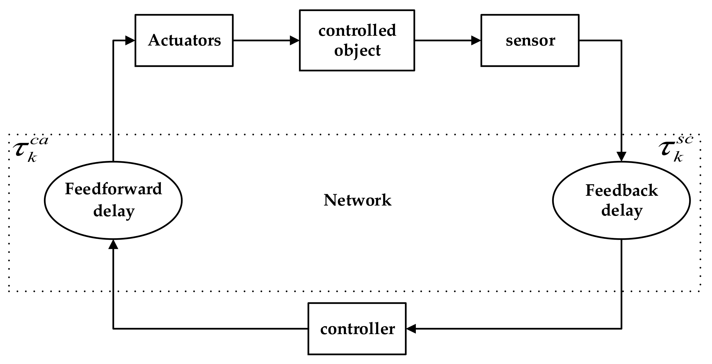
Figure 1. Structure of the network control system.
Applsci 13 00536 g001
Figure 2. Comparison of system response curves under different time delay.
Applsci 13 00536 g002
Figure 3. RBF neural network delay prediction model.
Applsci 13 00536 g003
Figure 4. Delay prediction model based on improved offline PSO-RBF network.
Applsci 13 00536 g004
Figure 5. The effect of the value of η on the control volume.
Applsci 13 00536 g005
Figure 6. Overall system architecture diagram.
Applsci 13 00536 g006
Figure 7. Measured time-delay sequence.
Applsci 13 00536 g007
Figure 8. Comparison of Optimal Search by PSO Algorithm Based on weight adjustment formulas.
Applsci 13 00536 g008
Figure 9. Comparison of forecasts from different forecasting algorithms, of which (a) shows the comparison of BP neural network prediction, (b) shows the comparison of RBF neural network prediction, and (c) shows the comparison of improved PSO-RBF neural network prediction.
Applsci 13 00536 g009aApplsci 13 00536 g009b
Figure 10. Error curves for different prediction algorithms.
Applsci 13 00536 g010
Figure 11. Network control system built with True-Time.
Applsci 13 00536 g011
Figure 12. Comparison of control effect.
Applsci 13 00536 g012
Figure 13. Sine signal following.
Applsci 13 00536 g013
Figure 14. Control error curve.
Applsci 13 00536 g014
Figure 15. Gaussian white noise.
Applsci 13 00536 g015
Figure 16. Comparison of control effects with interference signals.
Applsci 13 00536 g016
Figure 17. Physical validation platform.
Applsci 13 00536 g017
Figure 18. Physical verification comparison experiment.
Applsci 13 00536 g018
Table 1. Comparison of time-delay prediction evaluation metrics for different prediction algorithms.
Time-Delay Prediction MethodsRMSEMAECycle Forecast Time (ms)
BP Neural Networks0.02420.06885.47
RBF Neural Networks0.01880.20450.94
Improving PSO-RBF networks0.01050.03831.38
Table 2. Comparison of performance indicators of different controllers.
Control AlgorithmsIAEITAE
PID algorithms0.26160.2467
Fuzzy PID control0.11960.1069
RBF predictive control0.08310.0734
Table 3. Comparison of the performance of different controllers in the presence of interference signals.
Control AlgorithmsIAEITAE
PID algorithms0.31090.3623
Fuzzy PID control0.18260.1657
RBF predictive control0.12480.1196
Disclaimer/Publisher’s Note: The statements, opinions and data contained in all publications are solely those of the individual author(s) and contributor(s) and not of MDPI and/or the editor(s). MDPI and/or the editor(s) disclaim responsibility for any injury to people or property resulting from any ideas, methods, instructions or products referred to in the content.