Theoretical Model of Self-Magnetic Flux Leakage and Its Application in Estimating the Depth Direction of a Fatigue Crack

Featured Application

Compact proposal of theoretical model of self-magnetic flux leakage based on magnetic metal memory for estimating depth direction of a fatigue crack.

Abstract

In this study, theoretical models were proposed to explain the changes in self-magnetic flux density (SMFD) due to fatigue cracks in the presence and absence of external magnetic fields. Three theoretical models were proposed: rotation domain model (RDM), concentration domain model (CDM), and vertical domain model (VDM), considering the deformation and non-deformation possibilities. To prove the theoretical model, fatigue cracks with different depth angles were fabricated through fatigue testing and EDM processing on the CT specimens. In addition, tunnel magnetoresistance (TMR) sensors were used to evaluate the 3-axis distribution of SMFD. Comparing the simulation and experimental results, similar tendencies of the occurrence and depth angle of fatigue cracks and their effect on the distribution of SMFD were observed. According to the RDM, the distribution of SMFD occurs in the direction of the crack length (y-direction), while the CDM explains that the SMFD does not occur if the fatigue crack is in a direction perpendicular to the surface. In addition, the VDM shows that SMFDs occur in a direction perpendicular to the crack length (x-direction) and the specimen surface (z-direction). Interestingly, these trends agree with the experimental results, which confirms the validity of the theoretical model and thus can be used to estimate the depth direction of a fatigue crack.

1. Introduction

Large-scale building infrastructures, such as power generation facilities, railroads, bridges, and high-rise buildings, require extensive budgets and time investments. Therefore, social and economic benefits from investments can only be ensured when these infrastructures are operated with safety measures while maintaining the target performance throughout the design life. On the other hand, the damage-tolerant design states that a structure can be continuously operated even after the design life has elapsed if the target performance, safety, and economic feasibility are maintained. In this case, non-destructive (NDT) testing plays an important role to support defect detection. In damage tolerance engineering [1,2,3,4,5], determining tolerance size and appropriate maintenance and replacement are crucial factors. However, the stress concentration coefficients depend on the type of defects, such as voids, corrosion, fatigue cracks, delamination, and shelling, and consequently, the allowable tolerance sizes are different [6,7,8]. Therefore, it is essential to quantitatively evaluate the size and shape of the defects detected by NDT.

One of the challenges of NDT is detecting fatigue cracks that consist of a very thin crack layer. The initiation of fatigue crack on the metal and alloy is a convergence phenomenon that is influenced by many parameter interactions, physically and chemically. Widely known as damage accumulation, crack nucleation and growth occur when the local stress in the atomic displacement exceeds the yield strength of the material [9,10]. The accumulation of this displacement leads to continuous faults, such as deformation, dislocation motions, and evolution, in each atomic layer and initiates micro voids which transform into micro defects with high tendencies to grow with the applied loads. The fatigue crack can be initiated on the material surface or at an internal layer [11]. If fatigue cracks develop in a direction close to the normal to the surface, the structure will fracture rapidly. Furthermore, if fatigue cracks develop in a direction inclined parallel to the surface, the probability of delaminating or shelling increases. Therefore, it is important to evaluate the angle between the fatigue crack and the surface of the structure because this phenomenon can significantly reduce the life span of components and increase the probability of unexpected in-service failures [12]. Many approaches to NDT have been used to detect fatigue defects, one of which is surface defect detection.

In the case of a surface defect in NDT, large mechanical structures are detected using several methods such as visual, penetration, and magnetic particle testing, which can effectively determine the presence and length of a defect. However, it is difficult to implement these methods to evaluate the depth of the material defect [13]. A study on magnetic metal memory (MMM) has been reported in leakage magnetic flux testing which is able to detect an internal defect by measuring the self-magnetic flux leakage (SMFL) [14,15,16,17]. Many related studies have reported the development of this technology for solid ferromagnetic materials and assemblies of ferromagnetic materials, through experimental data models [18,19,20], the probability evaluation model [21], and the magnetic theoretical model. It was found that the SMFD signal around the defect changed depending on the defect types, defect position, and cross-sectional area [17].

Several studies have presented a theoretical equation for the leakage flux generated around a crack using a dipole model [22,23,24,25,26,27,28,29,30,31]. A formula was presented for the magnetization of a specimen by an external magnetic field, assuming that the magnetic dipole moment per unit area occurs at the crack surface. The formula has been used as a model that simulates the qualitative (and partially quantitative) change in MFL based on the presence of defects [22,23,24,25,26,27] and sensor designs [28,29], and is used for quantitative evaluation [22,23,24,25,26,27,29,30,31]. However, it is difficult to apply it to very narrow cracks, such as fatigue cracks. In addition, the change in the magnetic flux density (MFD) with the change in stress remains unclear, where conventional studies on MMM states that the magnetic flux density changes when stress changes or fatigue cracks occur, even when no external magnetic field is applied [32,33,34,35,36]. Therefore, it is uncoherent to use a magnetic dipole that assumes that an external magnetic field is applied which make the specimen in a magnetized state. Therefore, there is a need for a theoretical model to explain the SMFL phenomenon that plays the same role as the magnetic dipole model introduced in the MFLT and SMFL.

Furthermore, to formulate the theoretical model of MMM, several phenomena are considered. Wilson et al. [32] reported that, for applied stress measurements in the stress region of a steel sample, the magnetic field component parallel to the applied stress has a considerably greater correlation than the normal component. This is because of the magnetic field distribution in the stress region, which is related to the magnetic field distribution generated in the sample after the stress is released, and the pattern was confirmed experimentally. On the other hand, Berkache et al. [33] compared the stress analysis using the finite element method (FEM), measured the 3-axial magnetic flux density distribution, and examined the correlation. The stress distribution, which uses the parameter of the 3-axial magnetic flux density, was set as a qualitative relationship in the third polynomial formula. As a result, it was reported that it is possible to examine stress using the MMM. However, a quantitative evaluation of stress is accompanied by a large error. Kim et al. [34] derived a formula in which a change in stress accompanying mechanical deformation causes a change in SMFD. In addition, it was experimentally verified that a change in the SMFD distribution occurred owing to the change in the stress in the weld zone. A system for measuring the residual stress of a wide welding line with a high spatial resolution, using 64 GMR sensor elements arranged at intervals of 0.6 mm, was proposed. In addition to the review of stress performance and its effect on the MFD, the residual magnetic fields have also been considered. Roskosz et al. [35] investigated the residual magnetic field as a diagnostic signal for the reliable evaluation of the material. Accordingly, the possibility of defining the plastic deformation region of a component, determining the approximate distribution of stresses and strains, and defining the remaining lifespan of the component was presented. Finally, Dubov et al. [36] investigated the applicability of the metal magnetic memory (MMM) method for the stress–strain state (SSS) and NDT evaluation of gas and petroleum pipelines. Using the MMM method, it was suggested that the stress concentration zone (SCZ), where the development process of fatigue damage is intensively strengthened, can be detected and used to remove this zone. Unfortunately, despite the several studies on MMM presented above, it is challenging to develop a theoretical model to explain fatigue cracking and evaluate the depth direction of fatigue cracks by measuring the self-magnetization, and deciding whether the edge of the ferromagnetic metal structure is magnetized or the magnetic flux density shifted near fatigue crack despite the absence of external magnetic field.

Dealing with this gap, the change in magnetic domain caused by SSS and fatigue cracking with a narrow width was reviewed and modeled in this study. A valid domain model was selected to evaluate the depth direction inside fatigue cracks. The depth direction of the fatigue cracks was evaluated by measuring the MFD distribution based on the self-magnetization of the subject. Carbon steel specimens (SA 106) were subjected to fatigue crack tests using a compact tension (CT) specimen, and a small volume of 8 × 16 × 6.4 mm (width × length × height) containing the crack was cut with different cutting angles of 30, 60, and 90°. The MFD distribution on the surface of the specimen was measured using a 3-axis tunnel magneto-resistance (TMR) sensor. An evaluation algorithm for the depth direction was derived using the 3-axial SMFD distribution.

2. Magnetic Domain Models for Stress and Fatigue Cracks

Definition and statements of magnetic dipole moment ($\overrightarrow{\mathrm{m}}$), magnetization ($\overrightarrow{\mathrm{M}}$), magnetic flux density ($\overrightarrow{\mathrm{B}}$), vector magnetic potential ($\overrightarrow{\mathrm{A}}$), and magnetization surface current density (${\overrightarrow{\mathrm{J}}}_{\mathrm{ms}}$) are referred to as reference [37] in this paper. A magnetic dipole moment $\overrightarrow{\mathrm{m}}$, is assumed to be generated by electrons rotating and orbiting around the nucleus of a ferromagnetic metal. Regions with magnetic moments in the same direction are called magnetic domains and the boundaries of these regions are called domain walls. Magnetization $\overrightarrow{\mathrm{M}}$ is defined by Equation (1). Here, $∆\mathrm{v}$ is the micro-volume in the 3-dimensional model, and can be replaced by the micro-area $∆\mathrm{s}$ in the 2-dimensional model.

$$\overrightarrow{\mathrm{M}}=\underset{∆\mathrm{v}\to 0}{\lim }\frac{{\displaystyle \sum }_{\mathrm{k}=1}^{∆\mathrm{v}}{\overrightarrow{\mathrm{m}}}_{\mathrm{k}} }{∆\mathrm{v}}, (\mathrm{A}/\mathrm{m})$$

(1)

Figure 1a,b shows the rotation domain model (RDM) in which the magnetization is rotated. Figure 1c,d show a concentration domain model (CDM), which is arranged in the direction in which the magnetization is concentrated at the center. Figure 1e,f show the vertical domain model (VDM), where the magnetization is arranged in a direction perpendicular to the surface. RDM, CDM, and VDM are separate concepts from the domain theory of magnetism [38]. Figure 1a,c), 1e show a two-dimensional magnetic domain model with magnetizations ${\overrightarrow{\mathrm{M}}}_1$, ${\overrightarrow{\mathrm{M}}}_2$, ${\overrightarrow{\mathrm{M}}}_3$, and ${\overrightarrow{\mathrm{M}}}_4$ in each magnetic domain with areas S₁, S₂, S₃, and S₄ in a state where no external magnetic field $\overrightarrow{\mathrm{H}}$ is applied ($\overrightarrow{\mathrm{H}}=0$). In contrast, the equivalent magnetization ${\overrightarrow{\mathrm{M}}}_{\mathrm{eqv}}$ can be expressed as weighted average from the total surface area obtained by multiplying the magnetization by the corresponding area of the magnetic domain ${\mathrm{S}}_{\mathrm{k}}$ divided by total area of magnetic domain, as shown in Equation (2), when $\overrightarrow{\mathrm{H}}=0$, ${\overrightarrow{\mathrm{M}}}_{\mathrm{eqv}}=0$. In Equation (2), n is the number of magnetic domains. In this study, we specified n = 4 or n = 8 correspond to the number of models arrayed to the system.

$${\overrightarrow{\mathrm{M}}}_{\mathrm{eqv}}=\frac{1}{\mathrm{S}}{{\displaystyle \sum }}_{\mathrm{k}=1}^{\mathrm{n}}{\mathrm{S}}_{\mathrm{k}}{\overrightarrow{\mathrm{M}}}_{\mathrm{k}}, (\mathrm{A}/\mathrm{m})$$

(2)

$$\mathrm{S}={{\displaystyle \sum }}_{\mathrm{k}=1}^{\mathrm{n}}{\mathrm{S}}_{\mathrm{k}}, ({\mathrm{m}}^2)$$

(3)

When an external magnetic field $\overrightarrow{\mathrm{H}}$ is applied ($\overrightarrow{\mathrm{H}}\ne 0$), as shown in Figure 1d,e, the magnetic domain wall moves, and the area of the magnetic domain (S₂ or S₁) with a magnetic moment in the same direction as $\overrightarrow{\mathrm{H}}$ increases. In addition, the area of magnetization (S₄ or S₃) with a magnetic moment opposite to $\overrightarrow{\mathrm{H}}$ becomes smaller. Consequently, in the state where $\overrightarrow{\mathrm{H}}\ne 0$, ${\overrightarrow{\mathrm{M}}}_{\mathrm{eqv}}\ne 0$. However, in the VDM of Figure 1f, even when an external magnetic field $\overrightarrow{\mathrm{H}}$ is applied ($\overrightarrow{\mathrm{H}}\ne 0$), ${\overrightarrow{\mathrm{M}}}_{\mathrm{eqv}}=0$, so in the two-dimensional magnetic domain model, the changes of RDM and CDM are justifiable. The equivalent magnetization ${\overrightarrow{\mathrm{M}}}_{\mathrm{eqv}}$ can be expressed as the product of magnetic susceptibility ${\mathsf{\chi }}_{\mathrm{m}}$, which is an intrinsic property of a material, and the external magnetic field $\overrightarrow{\mathrm{H}}$, which is expressed in Equation (4).

$${\overrightarrow{\mathrm{M}}}_{\mathrm{eqv}}={\mathsf{\chi }}_{\mathrm{m}}\overrightarrow{\mathrm{H}}, (\mathrm{A}/\mathrm{m})$$

(4)

The magnetic susceptibility is not a constant entity, but corresponds to a parameter for an external magnetic field, which causes magnetic hysteresis. In other words, even after the external magnetic field is removed, the residual magnetization phenomenon of ${\overrightarrow{\mathrm{M}}}_{\mathrm{eqv}}\ne 0$ appears. In this state, for ${\overrightarrow{\mathrm{M}}}_{\mathrm{eqv}}=0$, an external magnetic field in the reverse direction, i.e., a coercive force, must be applied.

The MFD $\overrightarrow{\mathrm{B}}$ outside the ferromagnetic metal can be expressed as the superposition of the external magnetic field $\overrightarrow{\mathrm{H}}$ and the equivalent magnetization, as in Equation (5). Here, ${\mathsf{\mu }}_0$, ${\mathsf{\mu }}_{\mathrm{r}}$, and $\mathsf{\mu }$ are the permeability in free space, relative permeability, and permeability, respectively. According to Equation (5), when $\overrightarrow{\mathrm{H}}=0$, ${\overrightarrow{\mathrm{M}}}_{\mathrm{eqv}}=0$.

$$\overrightarrow{\mathrm{B}}={\mathsf{\mu }}_0\overrightarrow{\mathrm{H}}+{\mathsf{\mu }}_0{\overrightarrow{\mathrm{M}}}_{\mathrm{eqv}}={\mathsf{\mu }}_0\left(1+{\mathsf{\chi }}_{\mathrm{m}}\right)\overrightarrow{\mathrm{H}}={\mathsf{\mu }}_0{\mathsf{\mu }}_{\mathrm{r}}\overrightarrow{\mathrm{H}}=\mathsf{\mu }\overrightarrow{\mathrm{H}}, (\mathrm{Wb}/{\mathrm{m}}^2)$$

(5)

$${\mathsf{\mu }}_0=4\mathsf{\pi }\times {10}^{-7}, (\mathrm{H}/\mathrm{m})$$

(6)

Although it is not a magnetic hysteresis phenomenon, as shown in Figure 2, when a mechanical load is applied and deformation occurs, a phenomenon in which ${\overrightarrow{\mathrm{M}}}_{\mathrm{eqv}}\ne 0$ may occur at $\overrightarrow{\mathrm{H}}=0$. Figure 2a–c show conceptual diagrams applying RDM, CDM, and VDM, respectively, with n = 8 to a cantilever beam. Figure 2d–f show the deformation that occurred when a load $\overrightarrow{\mathrm{F}}$ was applied to the tip of the cantilever beam. The area S_k of each magnetic domain was deformed into S_k′ by the load $\overrightarrow{\mathrm{F}}$. The strain ${\mathsf{\epsilon }}_{\mathsf{\alpha }\mathsf{\beta }}$ in each area can be expressed using Equation (7). In addition, the stress ${\mathsf{\sigma }}_{\mathsf{\alpha }\mathsf{\beta }}$ in each area can be expressed using Equation (8). In this study, both the tensile and shear stresses are expressed as ${\mathsf{\sigma }}_{\mathsf{\alpha }\mathsf{\beta }}$, (Equation (8)), where E is the elastic modulus and $\mathsf{\alpha } \mathrm{or} \mathsf{\beta }$ refers to the $\mathrm{x}$ or $\mathrm{y}$ direction

$${\mathrm{S}}_{\mathrm{k}}^{\prime }={\mathsf{\epsilon }}_{\mathsf{\alpha }\mathsf{\beta },\mathrm{k}}{\mathrm{S}}_{\mathrm{k}}, ({\mathrm{m}}^2)$$

(7)

$${\mathsf{\sigma }}_{\mathsf{\alpha }\mathsf{\beta },\mathrm{k}}={\mathrm{E} \mathsf{\epsilon }}_{\mathsf{\alpha }\mathsf{\beta },\mathrm{k}}, (\mathrm{N}/{\mathrm{m}}^2)$$

(8)

In the state of Figure 2d,e, when $\overrightarrow{\mathrm{H}}=0$, the equivalent magnetization $\overrightarrow{\mathrm{M}}{}_{\mathrm{eqv}}^{\prime }$ and the magnetic flux density $\overrightarrow{\mathrm{B}}{}^{\prime }$ can be expressed by Equations (9) and (10), respectively. S is the sum of the total area. In addition, Equation (10) can be expressed as Equations (11) and (12) by substituting in Equations (7) and (8). This formula indicates that a change in strain or stress causes a change in magnetic flux density.

$$\overrightarrow{\mathrm{M}}{}_{\mathrm{eqv}}^{\prime }=\frac{1}{\mathrm{S}}{{\displaystyle \sum }}_{\mathrm{k}=1}^{\mathrm{n}}{\mathrm{S}}_{\mathrm{k}}{{}^{\prime }\overrightarrow{\mathrm{M}}}_{\mathrm{k}}{}^{\prime }, (\mathrm{A}/\mathrm{m})$$

(9)

$$\overrightarrow{\mathrm{B}}{}^{\prime }={\mathsf{\mu }}_0\overrightarrow{\mathrm{M}}{}_{\mathrm{eqv}}^{\prime }=\frac{{\mathsf{\mu }}_0}{\mathrm{S}}{{\displaystyle \sum }}_{\mathrm{k}=1}^{\mathrm{n}}{\mathrm{S}}_{\mathrm{k}}{{}^{\prime }\overrightarrow{\mathrm{M}}}_{\mathrm{k}}{}^{\prime }, (\mathrm{Wb}/{\mathrm{m}}^2)$$

(10)

$$\overrightarrow{\mathrm{B}}{}^{\prime }=\frac{{\mathsf{\mu }}_0}{\mathrm{S}}{{\displaystyle \sum }}_{\mathrm{k}=1}^{\mathrm{n}}{\mathsf{\epsilon }}_{\mathsf{\alpha }\mathsf{\beta },\mathrm{k}}{\mathrm{S}}_{\mathrm{k}}{{}^{\prime }\overrightarrow{\mathrm{M}}}_{\mathrm{k}}{}^{\prime }, (\mathrm{Wb}/{\mathrm{m}}^2)$$

(11)

$$\overrightarrow{\mathrm{B}}{}^{\prime }=\frac{{\mathsf{\mu }}_0}{\mathrm{SE}}{{\displaystyle \sum }}_{\mathrm{k}=1}^{\mathrm{n}}{\mathsf{\sigma }}_{\mathsf{\alpha }\mathsf{\beta },\mathrm{k}}{\mathrm{S}}_{\mathrm{k}}{{}^{\prime }\overrightarrow{\mathrm{M}}}_{\mathrm{k}}{}^{\prime }, (\mathrm{Wb}/{\mathrm{m}}^2)$$

(12)

Figure 3 shows an example of a 3-dimensional representation of the RDM model in Figure 2a by extending it in the direction perpendicular to the xy plane, that is, the z-direction. This gap can be expressed by separating regions S₁–S₄ and S₅–S₈ in Figure 2. Hereafter, the gap is collectively referred to as a crack. Figure 3b shows a magnetic domain model with cracks in the direction perpendicular to the surface of the specimen, and Figure 3c shows a magnetic domain model with slanted cracks while maintaining hexahedronal shape. Figure 3d shows a case in which the top surface of the magnetic domain is deformed to be horizontal to the xy plane and has an inclined crack. In each figure, ${\overrightarrow{\mathrm{a}}}_{\mathrm{n}}$ denotes the surface unit vector. In addition, the unit vectors in the x, y, and z directions are expressed as ${\overrightarrow{\mathrm{a}}}_{\mathrm{x}}$, ${\overrightarrow{\mathrm{a}}}_{\mathrm{y}}$, and ${\overrightarrow{\mathrm{a}}}_{\mathrm{z}}$. The magnetization surface current density (MSCD), ${\overrightarrow{\mathrm{J}}}_{\mathrm{ms}}$, represented by the dotted arrow, is related to the magnetization (${\overrightarrow{\mathrm{M}}}_{\mathrm{k}}$), represented by the solid arrow and Equation (13).

In addition, the relationship between the equivalent MSCD (${\overrightarrow{\mathrm{J}}}_{\mathrm{eqv},\mathrm{mn}}$) and the equivalent magnetization (${\overrightarrow{\mathrm{M}}}_{\mathrm{eqv},\mathrm{mn}}$) can be expressed by Equation (14). In the case where there is no external magnetic field ($\overrightarrow{\mathrm{H}}=0$) and when no deformation occurs (${\mathsf{\epsilon }}_{\mathsf{\alpha }\mathsf{\beta },\mathrm{k}}=0$), ${\overrightarrow{\mathrm{M}}}_{\mathrm{eqv},14}=\overrightarrow{0}$ and ${\overrightarrow{\mathrm{M}}}_{\mathrm{eqv},58}=\overrightarrow{0}$. This corresponds to the case shown in Figure 3a, where the equivalent magnetization ${\overrightarrow{\mathrm{M}}}_{\mathrm{eqv},35}$ by two adjacent magnetizations ${\overrightarrow{\mathrm{M}}}_3$ and ${\overrightarrow{\mathrm{M}}}_5$ is $\overrightarrow{0}$. Moreover, in the case of Figure 3b–d, assuming that there are continuous magnetic domains in the ±x and ±y directions, ${\overrightarrow{\mathrm{M}}}_{\mathrm{eqv},14}=\overrightarrow{0}$, ${\overrightarrow{\mathrm{M}}}_{\mathrm{eqv},58}=\overrightarrow{0}$. However, because the equivalent magnetization expressed in Equation (2) is a model limited to adjacent magnetic domains bordering the magnetic domain wall, the equivalent magnetization ${\overrightarrow{\mathrm{M}}}_{\mathrm{eqv},35}$ by ${\overrightarrow{\mathrm{M}}}_3$ and ${\overrightarrow{\mathrm{M}}}_5$ is not $\overrightarrow{0}$. At this time, MSCDs ${\overrightarrow{\mathrm{J}}}_3$ and ${\overrightarrow{\mathrm{J}}}_5$, are located at the interface of the crack.

$${\overrightarrow{\mathrm{J}}}_{\mathrm{ms},\mathrm{k}}={\overrightarrow{\mathrm{M}}}_{\mathrm{k}}\times {\overrightarrow{\mathrm{a}}}_{\mathrm{n},\mathrm{k}}, (\mathrm{A}/\mathrm{m})$$

(13)

$${\overrightarrow{\mathrm{J}}}_{\mathrm{eqv},\mathrm{mn}}={\overrightarrow{\mathrm{M}}}_{\mathrm{eqv},\mathrm{mn}}\times {\overrightarrow{\mathrm{a}}}_{\mathrm{eqv},\mathrm{mn}}, (\mathrm{A}/\mathrm{m})$$

(14)

Figure 3. Simplified 3-D magnetic domains: (a) without gap, (b) with gap, (c) with gradient gap without deformation, (d) with gradient gap with deformation.

Figure 3. Simplified 3-D magnetic domains: (a) without gap, (b) with gap, (c) with gradient gap without deformation, (d) with gradient gap with deformation.

Figure 4, Figure 5 and Figure 6 shows the simplified magnetization surface current densities on the RDM, CDM, and VDM. Figure 4 shows a schematic of ${\overrightarrow{\mathrm{J}}}_{\mathrm{k},\mathrm{edge}}$ and ${\overrightarrow{\mathrm{M}}}_{\mathrm{k},\mathrm{edge}}$ in the xz plane by RDM at the crack tip. When the width of the crack is w, Equation (13) can be expressed as Equation (15): Here, the intensity of ${\overrightarrow{\mathrm{M}}}_{\mathrm{k},\mathrm{edge}}$ is assumed to be ${\mathrm{M}}_0$. w and θ represent the crack width and inclination angle, respectively. $\mathrm{P}\left(\mathrm{x},\mathrm{h}-\mathrm{z}\right)$ represents a specific position at the top of the magnetic domain model. D is the depth of the crack, and h is the lift-off. Equation (15) is a general expression expressing all of Figure 3b–d.

$${\overrightarrow{\mathrm{J}}}_{\mathrm{RDM},\mathrm{k},\mathrm{edge}}={\mathrm{M}}_0\left({\sin \mathsf{\theta }\overrightarrow{\mathrm{a}}}_{\mathrm{x}}+{\cos \mathsf{\theta }\overrightarrow{\mathrm{a}}}_{\mathrm{z}}\right), (\mathrm{A}/\mathrm{m})$$

(15)

Figure 5 shows a schematic of ${\overrightarrow{\mathrm{J}}}_{\mathrm{k},\mathrm{edge}}$ and ${\overrightarrow{\mathrm{M}}}_{\mathrm{k},\mathrm{edge}}$ in the xz plane by CDM at the crack tip. According to the CDM domain model in the state in which the domain is not deformed, as shown in Figure 3c, Equation (13) can be expressed as Equation (16). This is generally represented as in Figure 5b,c. According to the CDM in the state in which the domain is deformed, as shown in Figure 5d, Equation (13) can be expressed as Equation (17).

$${\overrightarrow{\mathrm{J}}}_{\mathrm{CDM},\mathrm{k},\mathrm{edge}}=\overrightarrow{0}, (\mathrm{A}/\mathrm{m})$$

(16)

$${\overrightarrow{\mathrm{J}}{}^{\prime }}_{\mathrm{CDM},\mathrm{k},\mathrm{edge}}=-{\mathrm{M}}_0{\sin \mathsf{\theta }\overrightarrow{\mathrm{a}}}_{\mathrm{y}}, (\mathrm{A}/\mathrm{m})$$

(17)

Figure 5. Simplified magnetization surface current densities on the concentration domain model: (a) without gap, (b) with gap, (c) with gradient gap without deformation, (d) with gradient gap with deformation.

Figure 5. Simplified magnetization surface current densities on the concentration domain model: (a) without gap, (b) with gap, (c) with gradient gap without deformation, (d) with gradient gap with deformation.

Figure 6 is a schematic of ${\overrightarrow{\mathrm{J}}}_{\mathrm{k},\mathrm{edge}}$ and ${\overrightarrow{\mathrm{M}}}_{\mathrm{k},\mathrm{edge}}$ in the xz-plane by VDM at the crack tip. According to the VDM in the state in which the magnetic domain is not deformed, as shown in Figure 3c, Equation (13) can be expressed as Equation (18). This is generally represented by Figure 6b,c. According to the VDM in the state in which the magnetic domain is deformed, as shown in Figure 6d, Equation (13) can be expressed as Equation (19).

$${\overrightarrow{\mathrm{J}}}_{\mathrm{VDM},\mathrm{k},\mathrm{edge}}={\mathrm{M}}_0{\overrightarrow{\mathrm{a}}}_{\mathrm{y}}, (\mathrm{A}/\mathrm{m})$$

(18)

$${\overrightarrow{\mathrm{J}}{}^{\prime }}_{\mathrm{VDM},\mathrm{k},\mathrm{edge}}={\mathrm{M}}_0{\cos \mathsf{\theta }\overrightarrow{\mathrm{a}}}_{\mathrm{y}}, (\mathrm{A}/\mathrm{m})$$

(19)

Figure 6. Simplified magnetization surface current densities on the vertical domain model: (a) without gap, (b) with gap, (c) with gradient gap without deformation, (d) with gradient gap with deformation.

Figure 6. Simplified magnetization surface current densities on the vertical domain model: (a) without gap, (b) with gap, (c) with gradient gap without deformation, (d) with gradient gap with deformation.

The vector magnetic potential (VMP) ($\overrightarrow{\mathrm{A}}$) and MFD ($\overrightarrow{\mathrm{B}}$) are expressed by Equations (20) and (21), respectively. In RDM, if the magnetic domain model is not subjected to an external load, $\overrightarrow{\mathrm{A}}$ can be expressed by Equations (22)–(24), where ${\overrightarrow{\mathrm{R}}}_3$ and ${\overrightarrow{\mathrm{R}}}_5$ represent the position vectors from the crack wall to a specific position, P(x,h).

$$\mathrm{d}\overrightarrow{\mathrm{A}}=\frac{{\mathsf{\mu }}_0}{4\mathsf{\pi }}{{\displaystyle \int }}_{{\mathrm{C}}^{\prime }}^{}\frac{\overrightarrow{\mathrm{J}}}{\mathrm{R}}{\mathrm{dl}}^{\prime }, (\mathrm{Wb}/\mathrm{m})$$

(20)

$$\mathrm{d}\overrightarrow{\mathrm{B}}=\nabla \times \mathrm{d}\overrightarrow{\mathrm{A}}, (\mathrm{Wb}/{\mathrm{m}}^2)$$

(21)

$${\mathrm{d}\overrightarrow{\mathrm{A}}}_{\mathrm{RDM}}\left(\mathrm{x},\mathrm{h}\right)=\frac{{\mathsf{\mu }}_0{\mathrm{M}}_0}{4\mathsf{\pi }}{{\displaystyle \int }}_{{\mathrm{C}}^{\prime }}^{}\left(\frac{1}{{\mathrm{R}}_3}+\frac{1}{{\mathrm{R}}_5}\right)\left({\sin \mathsf{\theta }\overrightarrow{\mathrm{a}}}_{\mathrm{x}}+{\cos \mathsf{\theta }\overrightarrow{\mathrm{a}}}_{\mathrm{z}}\right){\mathrm{dy}}^{\prime }$$

(22)

$${\mathrm{R}}_3=\sqrt{{\left(\mathrm{h}-\mathrm{z}\right)}^2+{\left(\frac{\mathrm{w}}{2}+\mathrm{x}\right)}^2}$$

(23)

$${\mathrm{R}}_5=\sqrt{{\left(\mathrm{h}-\mathrm{z}\right)}^2+{\left(\frac{\mathrm{w}}{2}-\mathrm{x}\right)}^2}$$

(24)

The unit area per VMPs, ${\overrightarrow{\mathrm{A}}}_{\mathrm{RDM},\mathrm{a}}$, ${\overrightarrow{\mathrm{A}}}_{\mathrm{RDM},\mathrm{b}}$, and ${\overrightarrow{\mathrm{A}}}_{\mathrm{RDM},\mathrm{c}}$ for each case of RDM shown in Figure 4a, b and c can be expressed by Equations (25)–(27), respectively. In Equation (27), w = 0 and θ = 0° can be expressed by Equations (25) and (26), respectively. Therefore, Equation (27) is a general formula that includes the cases with and without cracks. In addition, as shown in Figure 3d, inclined cracks caused by the undeformed and deformed RDMs are expressed in the same manner as in Equations (27) and (28), respectively. Therefore, MFD ($\overrightarrow{\mathrm{B}}$) in the RDM can be interpreted using Equations (29) and (30).

$${\mathrm{d}\overrightarrow{\mathrm{A}}}_{\mathrm{RDM},\mathrm{a}}\left(\mathrm{x},\mathrm{z}\right)=\overrightarrow{0}$$

(25)

$${\mathrm{d}\overrightarrow{\mathrm{A}}}_{\mathrm{RDM},\mathrm{b}}\left(\mathrm{x},\mathrm{h}\right)=\frac{{\mathsf{\mu }}_0{\mathrm{M}}_0}{4\mathsf{\pi }}\left(\frac{1}{{\mathrm{R}}_3}+\frac{1}{{\mathrm{R}}_5}\right){\overrightarrow{\mathrm{a}}}_{\mathrm{z}}$$

(26)

$${\mathrm{d}\overrightarrow{\mathrm{A}}}_{\mathrm{RDM},\mathrm{c}}\left(\mathrm{x},\mathrm{h}\right)=\frac{{\mathsf{\mu }}_0{\mathrm{M}}_0}{4\mathsf{\pi }}\left(\frac{1}{{\mathrm{R}}_3}+\frac{1}{{\mathrm{R}}_5}\right)\left({\sin \mathsf{\theta }\overrightarrow{\mathrm{a}}}_{\mathrm{x}}+{\cos \mathsf{\theta }\overrightarrow{\mathrm{a}}}_{\mathrm{z}}\right)$$

(27)

$${\mathrm{d}\overrightarrow{\mathrm{A}}}_{\mathrm{RDM},\mathrm{d}}\left(\mathrm{x},\mathrm{h}\right)=\frac{{\mathsf{\mu }}_0{\mathrm{M}}_0}{4\mathsf{\pi }}\left(\frac{1}{{\mathrm{R}}_3}+\frac{1}{{\mathrm{R}}_5}\right)\left({\sin \mathsf{\theta }\overrightarrow{\mathrm{a}}}_{\mathrm{x}}+{\cos \mathsf{\theta }\overrightarrow{\mathrm{a}}}_{\mathrm{z}}\right)$$

(28)

$${\mathrm{d}\overrightarrow{\mathrm{B}}}_{\mathrm{RDM}}\left(\mathrm{x},\mathrm{h}\right)=\frac{{\mathsf{\mu }}_0{\mathrm{M}}_0}{4\mathsf{\pi }}\left\{\left(\frac{\frac{\mathrm{w}}{2}+\mathrm{x}}{{\mathrm{R}}_3{}^3}-\frac{\frac{\mathrm{w}}{2}-\mathrm{x}}{{\mathrm{R}}_5{}^3}\right)\cos \mathsf{\theta }+\left(\frac{\mathrm{h}-\mathrm{z}}{{\mathrm{R}}_3{}^3}+\frac{\mathrm{h}-\mathrm{z}}{{\mathrm{R}}_5{}^3}\right)\sin \mathsf{\theta }\right\}{\overrightarrow{\mathrm{a}}}_{\mathrm{y}}$$

(29)

$${\overrightarrow{\mathrm{B}}}_{\mathrm{RDM}}\left(\mathrm{x},\mathrm{h}\right)={{\displaystyle \int }}_0^{\mathrm{D}}{\mathrm{d}\overrightarrow{\mathrm{B}}}_{\mathrm{RDM}}\mathrm{dz}$$

(30)

In CDM, $\overrightarrow{\mathrm{A}}$ is interpreted using Equations (31)–(34). The ${\overrightarrow{\mathrm{B}}}_{\mathrm{CDM},\mathrm{c}}$ by inclined cracks in the non-deformed CDM, is expressed by Equation (35). The ${\overrightarrow{\mathrm{B}}}_{\mathrm{CDM},\mathrm{d}}$ for cracks analyzed using the deformed CDM is interpreted as Equation (36) and (37).

$${\mathrm{d}\overrightarrow{\mathrm{A}}}_{\mathrm{CDM},\mathrm{a}}\left(\mathrm{x},\mathrm{z}\right)=\overrightarrow{0}$$

(31)

$${\mathrm{d}\overrightarrow{\mathrm{A}}}_{\mathrm{CDM},\mathrm{b}}\left(\mathrm{x},\mathrm{z}\right)=\overrightarrow{0}$$

(32)

$${\mathrm{d}\overrightarrow{\mathrm{A}}}_{\mathrm{CDM},\mathrm{c}}\left(\mathrm{x},\mathrm{z}\right)=\overrightarrow{0}$$

(33)

$${\mathrm{d}\overrightarrow{\mathrm{A}}}_{\mathrm{CDM},\mathrm{d}}\left(\mathrm{x},\mathrm{z}\right)=-\frac{{\mathsf{\mu }}_0{\mathrm{M}}_0}{4\mathsf{\pi }}\left(\frac{1}{{\mathrm{R}}_3}+\frac{1}{{\mathrm{R}}_5}\right){\sin \mathsf{\theta }\overrightarrow{\mathrm{a}}}_{\mathrm{y}}$$

(34)

$${\mathrm{d}\overrightarrow{\mathrm{B}}}_{\mathrm{CDM},\mathrm{c}}\left(\mathrm{x},\mathrm{z}\right)=\overrightarrow{0}$$

(35)

$${\mathrm{d}\overrightarrow{\mathrm{B}}}_{\mathrm{CDM},\mathrm{d}}\left(\mathrm{x},\mathrm{z}\right)=\frac{{\mathsf{\mu }}_0{\mathrm{M}}_0}{4\mathsf{\pi }}\left\{\left(\frac{\mathrm{h}-\mathrm{z}}{{\mathrm{R}}_3{}^3}+\frac{\mathrm{h}-\mathrm{z}}{{\mathrm{R}}_5{}^3}\right){\sin \mathsf{\theta }\overrightarrow{\mathrm{a}}}_{\mathrm{x}}+\left(\frac{\frac{\mathrm{w}}{2}+\mathrm{x}}{{\mathrm{R}}_3{}^3}-\frac{\frac{\mathrm{w}}{2}-\mathrm{x}}{{\mathrm{R}}_5{}^3}\right){\sin \mathsf{\theta }\overrightarrow{\mathrm{a}}}_{\mathrm{z}}\right\}$$

(36)

$${\overrightarrow{\mathrm{B}}}_{\mathrm{CDM},\mathrm{d}}\left(\mathrm{x},\mathrm{h}\right)={{\displaystyle \int }}_0^{\mathrm{D}}{\mathrm{d}\overrightarrow{\mathrm{B}}}_{\mathrm{CDM},\mathrm{d}}\mathrm{dz}$$

(37)

Equations (38)–(41) show $\overrightarrow{\mathrm{A}}$ in VDM. The MFDs (${\overrightarrow{\mathrm{B}}}_{\mathrm{VDM},\mathrm{c}}$, ${\overrightarrow{\mathrm{B}}}_{\mathrm{VDM},\mathrm{d}}$) generated around the slanted crack caused by the non-deformed and deformed VDM are interpreted by Equations (42) and (43), and Equations (44) and (45), respectively.

$${\mathrm{d}\overrightarrow{\mathrm{A}}}_{\mathrm{VDM},\mathrm{a}}\left(\mathrm{x},\mathrm{z}\right)=\overrightarrow{0}$$

(38)

$${\mathrm{d}\overrightarrow{\mathrm{A}}}_{\mathrm{VDM},\mathrm{b}}\left(\mathrm{x},\mathrm{z}\right)=\frac{{\mathsf{\mu }}_0{\mathrm{M}}_0}{4\mathsf{\pi }}\left(\frac{1}{{\mathrm{R}}_3}+\frac{1}{{\mathrm{R}}_5}\right){\overrightarrow{\mathrm{a}}}_{\mathrm{y}}$$

(39)

$${\mathrm{d}\overrightarrow{\mathrm{A}}}_{\mathrm{VDM},\mathrm{c}}\left(\mathrm{x},\mathrm{z}\right)=\frac{{\mathsf{\mu }}_0{\mathrm{M}}_0}{4\mathsf{\pi }}\left(\frac{1}{{\mathrm{R}}_3}+\frac{1}{{\mathrm{R}}_5}\right){\overrightarrow{\mathrm{a}}}_{\mathrm{y}}$$

(40)

$${\mathrm{d}\overrightarrow{\mathrm{A}}}_{\mathrm{VDM},\mathrm{d}}\left(\mathrm{x},\mathrm{z}\right)=\frac{{\mathsf{\mu }}_0{\mathrm{M}}_0}{4\mathsf{\pi }}\left(\frac{1}{{\mathrm{R}}_3}+\frac{1}{{\mathrm{R}}_5}\right){\cos \mathsf{\theta }\overrightarrow{\mathrm{a}}}_{\mathrm{y}}$$

(41)

$${\mathrm{d}\overrightarrow{\mathrm{B}}}_{\mathrm{VDM},\mathrm{c}}\left(\mathrm{x},\mathrm{z}\right)=-\frac{{\mathsf{\mu }}_0{\mathrm{M}}_0}{4\mathsf{\pi }}\left\{\left(\frac{\mathrm{h}-\mathrm{z}}{{\mathrm{R}}_3{}^3}+\frac{\mathrm{h}-\mathrm{z}}{{\mathrm{R}}_5{}^3}\right){\overrightarrow{\mathrm{a}}}_{\mathrm{x}}+\left(\frac{\frac{\mathrm{w}}{2}+\mathrm{x}}{{\mathrm{R}}_3{}^3}-\frac{\frac{\mathrm{w}}{2}-\mathrm{x}}{{\mathrm{R}}_5{}^3}\right){\overrightarrow{\mathrm{a}}}_{\mathrm{z}}\right\}$$

(42)

$${\overrightarrow{\mathrm{B}}}_{\mathrm{VDM},\mathrm{c}}\left(\mathrm{x},\mathrm{h}\right)={{\displaystyle \int }}_0^{\mathrm{D}}{\mathrm{d}\overrightarrow{\mathrm{B}}}_{\mathrm{VDM},\mathrm{c}}\mathrm{dz}$$

(43)

$${\mathrm{d}\overrightarrow{\mathrm{B}}}_{\mathrm{VDM},\mathrm{d}}\left(\mathrm{x},\mathrm{z}\right)=-\frac{{\mathsf{\mu }}_0{\mathrm{M}}_0}{4\mathsf{\pi }}\left\{\left(\frac{\mathrm{h}-\mathrm{z}}{{\mathrm{R}}_3{}^3}+\frac{\mathrm{h}-\mathrm{z}}{{\mathrm{R}}_5{}^3}\right){\cos \mathsf{\theta }\overrightarrow{\mathrm{a}}}_{\mathrm{x}}+\left(\frac{\frac{\mathrm{w}}{2}+\mathrm{x}}{{\mathrm{R}}_3{}^3}-\frac{\frac{\mathrm{w}}{2}-\mathrm{x}}{{\mathrm{R}}_5{}^3}\right){\cos \mathsf{\theta }\overrightarrow{\mathrm{a}}}_{\mathrm{z}}\right\}$$

(44)

$${\overrightarrow{\mathrm{B}}}_{\mathrm{VDM},\mathrm{d}}\left(\mathrm{x},\mathrm{h}\right)={{\displaystyle \int }}_0^{\mathrm{D}}{\mathrm{d}\overrightarrow{\mathrm{B}}}_{\mathrm{VDM},\mathrm{d}}\mathrm{dz}$$

(45)

In the RDM by Equation (29), when cracks occur, only the MFD of the y-component exists regardless of the deformation of the magnetic domain. In the undeformed CDM model, Equation (35), the MFD does not change, even if cracks occur. However, in the deformed CDM model according to Equation (36), when an inclined crack occurs, the MFDs in the x- and z-components change. In the undeformed VDM model using Equation (42), the MFD of the x- and z-components changes regardless of the inclination direction of the crack. In addition, in the deformed VDM model in the inclined crack according to Equation (44), the MFDs in the x- and z-components change. Moreover, the intensity of the MFD increases as the inclination angle θ of the crack approaches 0°.

Figure 7 shows a graph expressing the components in each direction expressed by Equation (29) according to the depth direction of the crack. To understand the qualitative trend, it was assumed that ${\mathrm{M}}_0=-4\mathsf{\pi }/{\mathsf{\mu }}_0$, h = 0.2 mm, w = 0.01 mm, and D = 5 mm. The y-component of ${\overrightarrow{\mathrm{B}}}_{\mathrm{RDM},\mathrm{c}}$ according to Figure 7 has a positive sign on the left and a negative sign on the right, near the crack center. As the angle of the crack increases, the negative maximum value on the right-side increases. In ${\overrightarrow{\mathrm{B}}}_{\mathrm{CDM},\mathrm{d}}$, according to Figure 8, only the x- and z-components appear, and when $\mathsf{\theta }=0{}^{°}$, the magnetic flux density is 0. In addition, in ${\overrightarrow{\mathrm{B}}}_{\mathrm{CDM},\mathrm{c}}$ by Equation (35), the magnetic flux density does not change. In ${\overrightarrow{\mathrm{B}}}_{\mathrm{VDM},\mathrm{c}}$ according to Figure 9, only the x- and z-components appear, and the magnitude of the absolute value increases with the angle. Because the length in the oblique direction increases for the same depth, a larger value appears as the inclination angle increases. However, the x-component indicates the maximum value in the vicinity of the crack and shows a symmetrical distribution. Further, the z-component has a negative maximum value on the left, centered on the maximum value of the x-component, indicating a distribution opposite to the y-component of ${\overrightarrow{\mathrm{B}}}_{\mathrm{RDM},\mathrm{c}}$ (Figure 7). In ${\overrightarrow{\mathrm{B}}}_{\mathrm{VDM},\mathrm{d}}$ shown in Figure 10, only the x- and z-components appear, and the x- and z-components that decrease in inverse proportion to the size of the angle can be observed. Furthermore, these results will form the theoretical model for estimating the depth direction of a fatigue crack. This trend is compared to the experimental results mentioned in the next section.

3. Materials and Methods

3.1. Specimen with Fatigue Crack

Fatigue crack specimens were prepared to investigate the validity of the proposed magnetic domain model and the change in MFD distribution according to the crack inclination angle. Figure 11 shows a schematic of the extraction of fatigue specimens from compact test (CT) specimens with fatigue cracks. A fatigue crack with a depth of 3–7 mm was created by applying a repeated load of 350–3500 N, 630,000–1,080,000 times to a CT specimen made of SS400 carbon steel with the dimensions 32 × 30.72 × 12.8 mm. As shown in Figure 12, small specimens of 6.4 × 16 × 8 mm were machined at different cutting angles by electric discharge machining (EDM). Consequently, each specimen contained fatigue cracks inclined at 0, 30, and 60°. Figure 13 shows the micrographs of the surface and side of each specimen. Each specimen was polished using 200, 400, 800, 1200, and 2000 grades SiC pads. Finally, fine polishing was performed for 20 s using polycrystalline diamond paste with a lattice size of 1 μm and a polishing cloth. After micro-polishing was completed, an etching solution prepared by diluting 3 g of nitric acid in 65 g of ethanol was applied to the observation surface for 5 s, followed by ultrasonic cleaning with distilled water for 15 s and washing with ethanol for 10 s. After repeating this chemical etching thrice, it was photographed with an optical microscope, and the 3-axial MFD was measured at a lift-off of 0.2 mm.

3.2. Measurement of Magnetic Flux Density with 3-Axis TMR Sensor Scanning

Figure 14a shows the experimental setup for measuring the MFD distribution on the upper part of each specimen using a 3-axis TMR sensor. A microscope and a 3-axis TMR sensor were installed on an optical board. Figure 14b shows an enlarged photograph of the red square in Figure 14a. The specimen was fixed with a key to reproduce the absolute positions of the optical images and TMR scanning before and after polishing. In addition, the specimen fixed by the key measured the MFD distribution with a spatial resolution of 4 μm and acquired an optical microscope image using a motorized XY stage. The MFD distribution was measured using a 3-axis TMR sensor (TMR2305, Multidimension Co., Paris, France). The sensitivity of each sensor was 25 mV/V/Oe, and the saturation magnetic field was ±10 Oe. As a result of amplification by 46 dB (200 times) by the signal processing circuit, 1 V is the output for an MFD of 0.2 G. The distance between the surface of the specimen and the sensor surface and the lift-off was maintained at approximately 0.2 mm.

4. Experimental Results

Training, testing, and analysis processes were performed using MATLAB R2021a software on a Dell ALIENWARE PC with an Intel® Core™ i9-9900HQ 3.6 GHz of CPU and 32 GB of RAM. Several positive results were achieved in this study and a theoretical model of magnetic metal memory was proposed to estimate the depth direction of a fatigue crack (see Figure 7, Figure 8 and Figure 9). To provide a comparison, an experiment was conducted using a 3-axis TMR sensor on CT scan specimens with fatigue cracks on three variations of depth angle: $0^{\mathrm{o}}$, ${30}^{\mathrm{o}}$, and ${60}^{\mathrm{o}}$. In addition, to maintain the validity of the measurement, the experiment was conducted on a wide demagnetized aluminum plate to reduce the probability of an external magnetic field disturbing the recorded dataset.

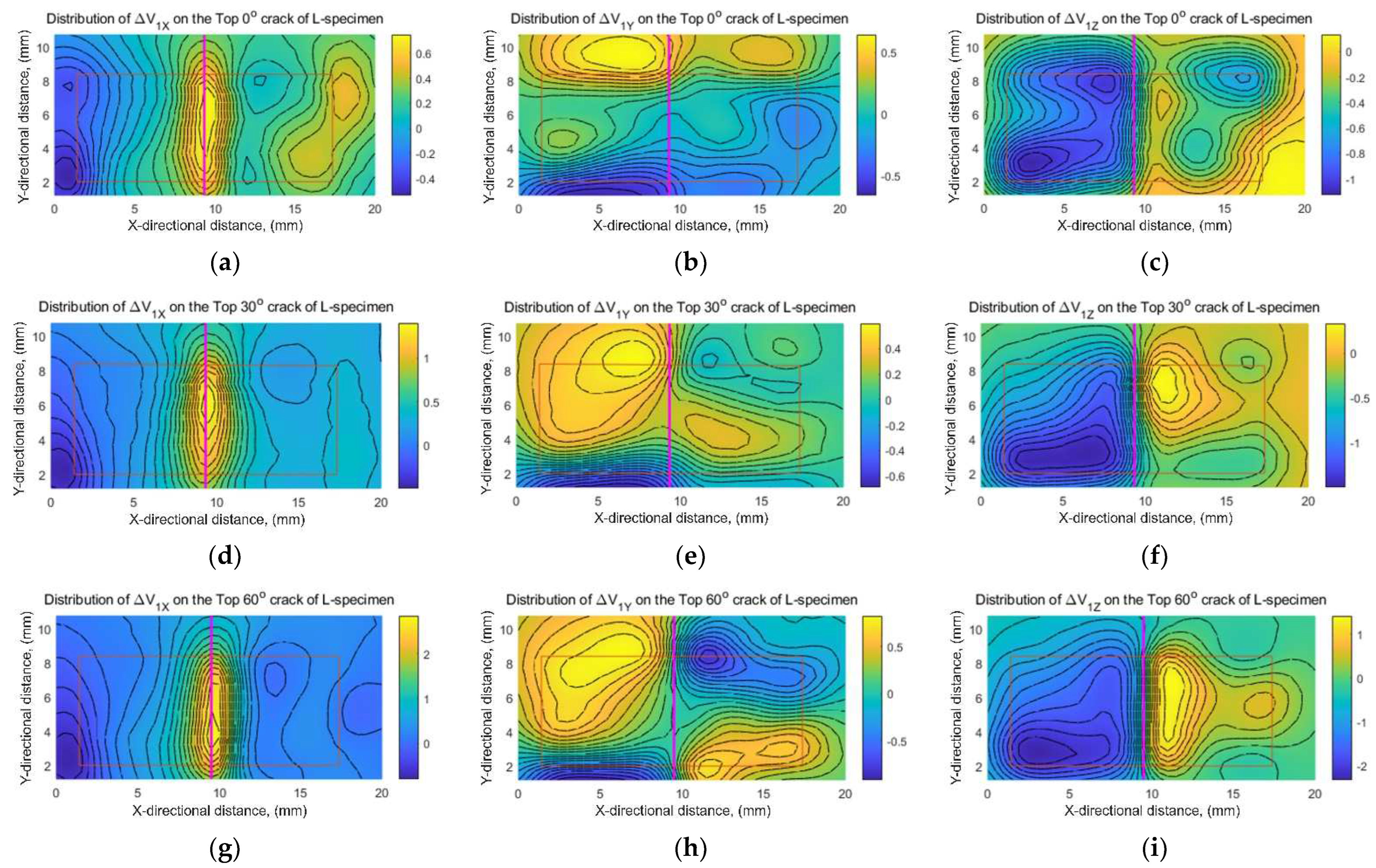
Figure 15 shows the raw output signal of the 3-axis TMR sensor in the x- (${\mathrm{V}}_{\mathrm{raw},\mathrm{X}}$), y- (${\mathrm{V}}_{\mathrm{raw},\mathrm{Y}}$), and z- (${\mathrm{V}}_{\mathrm{raw},\mathrm{Z}}$) directions. To map the distribution of the magnetic fields, the contour lines are added to all of the variations. In addition, the coordination of the specimen boundaries and the centerline line of the fatigue cracks are represented by the brown box and thick pink line on the vertical axis. The upper part of the rectangle is the surface side of the CT specimen, and the lower part is the center surface which is cut by EDM processes. To provide clear data for supporting the analysis, signal processing was conducted. The idea is to delete the background distribution of SMFD data by subtracting the raw data (${\overrightarrow{\mathrm{V}}}_{\mathrm{raw}}\left(\mathrm{x},\mathrm{y}\right)$) from the background distribution (${\overrightarrow{\mathrm{V}}}_{\mathrm{back}}\left(\mathrm{x},\mathrm{y}\right)$). The ${\overrightarrow{\mathrm{V}}}_{\mathrm{back}}\left(\mathrm{x},\mathrm{y}\right)$ was gathered by measuring the distribution of SMFD in the air by removing the specimen from the setup. The signal processing processes can be described mathematically as follow:

$$∆{\overrightarrow{\mathrm{V}}}_1\left(\mathrm{x},\mathrm{y}\right)={\overrightarrow{\mathrm{V}}}_{\mathrm{raw}}\left(\mathrm{x},\mathrm{y}\right)-{\overrightarrow{\mathrm{V}}}_{\mathrm{back}}\left(\mathrm{x},\mathrm{y}\right)$$

(46)

$${\overrightarrow{\mathrm{V}}}_{\mathrm{raw}}\left(\mathrm{x},\mathrm{y}\right)={\mathrm{V}}_{\mathrm{raw},\mathrm{X}}\left(\mathrm{x},\mathrm{y}\right){\overrightarrow{\mathrm{a}}}_{\mathrm{x}}+{\mathrm{V}}_{\mathrm{raw},\mathrm{Y}}\left(\mathrm{x},\mathrm{y}\right){\overrightarrow{\mathrm{a}}}_{\mathrm{y}}+{\mathrm{V}}_{\mathrm{raw},\mathrm{Z}}\left(\mathrm{x},\mathrm{y}\right){\overrightarrow{\mathrm{a}}}_{\mathrm{Z}}$$

(47)

$${\overrightarrow{\mathrm{V}}}_{\mathrm{back}}\left(\mathrm{x},\mathrm{y}\right)={\mathrm{V}}_{\mathrm{back},\mathrm{X}}\left(\mathrm{x},\mathrm{y}\right){\overrightarrow{\mathrm{a}}}_{\mathrm{x}}+{\mathrm{V}}_{\mathrm{back},\mathrm{Y}}\left(\mathrm{x},\mathrm{y}\right){\overrightarrow{\mathrm{a}}}_{\mathrm{y}}+{\mathrm{V}}_{\mathrm{back},\mathrm{Z}}\left(\mathrm{x},\mathrm{y}\right){\overrightarrow{\mathrm{a}}}_{\mathrm{Z}}$$

(48)

where, Figure 16 shows the distribution of Equation (46) and corresponds to the background signal in the x- (${\mathrm{V}}_{\mathrm{back},\mathrm{x}}$), y- (${\mathrm{V}}_{\mathrm{back},\mathrm{Y}}$), and z- (${\mathrm{V}}_{\mathrm{back},\mathrm{Z}}$) directions. Interestingly, the overall trends in each case in Figure 15 and Figure 16 are very similar, indicating that the external magnetic field has negligible effect on the experimental values. As shown in Figure 16a,d,g, the X-component, $∆{\mathrm{V}}_{1,\mathrm{X}}$, has a maximum value near the center of the crack, regardless of the depth angle of the crack, and has a symmetrical shape. As shown in Figure 16c,f,i, the Z-component, $∆{\mathrm{V}}_{1,\mathrm{Z}}$, represents the distribution of the different signs on the left and right sides around the crack. This phenomenon can be explained by the VDM in Figure 9 and Figure 10. Moreover, as shown in Figure 16b,e,h, the Y-component, $∆{\mathrm{V}}_{1,\mathrm{Y}}$, does not differ significantly along the center line of the crack, indicating that the VDM model is valid.

To investigate the quantitative trend of MFD based on the angle direction to the depth of cracks, Figure 17, Figure 18 and Figure 19 show the MFD distribution along a line passing through the center of the specimen (y = 5.1 mm) in Figure 15 and Figure 16. In each graph, $∆{\overrightarrow{\mathrm{V}}}_2\left(\mathrm{x},\mathrm{y}\right)$ is the value expressed by Equation (49). $∆{\overrightarrow{\mathrm{V}}}_{1, \mathrm{avr}}\left(\mathrm{x},\mathrm{y}\right)$ is the average value expressed by Equation (50). This variable was introduced to observe the correlation between the position of x and the crack inclination angle when $∆{\overrightarrow{\mathrm{V}}}_2\left(\mathrm{x},\mathrm{y}\right)=0$. In addition, M, N, and r are the number of data points in the x-axis direction (M = 5000), number of data points in the y-axis direction (N = 2500), and spatial resolution (r = 0.004 mm), respectively. The thick solid line near the center of the longitudinal axis (x = 9.3–9.5 mm) is the central position of the crack observed under the microscope. The solid vertical lines at x = 1.4 mm and x = 15.9 mm indicate the positions of both corners of the specimen.

$$∆{\overrightarrow{\mathrm{V}}}_2\left(\mathrm{x},\mathrm{y}\right)=∆{\overrightarrow{\mathrm{V}}}_1\left(\mathrm{x},\mathrm{y}\right)-∆{\overrightarrow{\mathrm{V}}}_{1, \mathrm{avr}}\left(\mathrm{x},\mathrm{y}\right)$$

(49)

$$∆{\overrightarrow{\mathrm{V}}}_{1,\mathrm{avr}}\left(\mathrm{x},\mathrm{y}\right)=\frac{1}{\mathrm{MN}}\left({\displaystyle \sum }_{\mathrm{i}=1}^{\mathrm{M}}{\displaystyle \sum }_{\mathrm{j}=1}^{\mathrm{N}}{\mathrm{V}}_{1,\mathrm{X}}\left(\mathrm{ir},\mathrm{jr}\right){\overrightarrow{\mathrm{a}}}_{\mathrm{x}}+{\displaystyle \sum }_{\mathrm{i}=1}^{\mathrm{M}}{\displaystyle \sum }_{\mathrm{j}=1}^{\mathrm{N}}{\mathrm{V}}_{1,\mathrm{Y}}\left(\mathrm{ir},\mathrm{jr}\right){\overrightarrow{\mathrm{a}}}_{\mathrm{y}}+{\displaystyle \sum }_{\mathrm{i}=1}^{\mathrm{M}}{\displaystyle \sum }_{\mathrm{j}=1}^{\mathrm{N}}{\mathrm{V}}_{1,\mathrm{Z}}\left(\mathrm{ir},\mathrm{jr}\right){\overrightarrow{\mathrm{a}}}_{\mathrm{Z}}\right)$$

(50)

Comparing ${\mathrm{V}}_{\mathrm{raw},\mathrm{x}}\left(\mathrm{x},5.1\right)$ in Figure 17a and $∆{\mathrm{V}}_{1,\mathrm{x}}\left(\mathrm{x},5.1\right)$ in Figure 17b, the background signal of about −0.9 V (approximately −0.18 G) is applied uniformly. As the overall depth angle increased, the peak value also increased. This means that ${\overrightarrow{\mathrm{B}}}_{\mathrm{CDM},\mathrm{c}}\left(\mathrm{x},\mathrm{z}\right)$ in Figure 9 exhibits a more accurate trend than ${\overrightarrow{\mathrm{B}}}_{\mathrm{CDM},\mathrm{d}}\left(\mathrm{x},\mathrm{z}\right)$ in Figure 10, i.e., for the same depth, the area of magnetization widens according to the inclination angle, which means that a larger MFD distribution is obtained as a result.

In contrast, the position of the peak was deflected to the right (direction with an acute angle) according to the depth angle. Therefore, if the central position of the crack can be specified by penetrant inspection, the crack direction to depth based on the correlation with the peak position can be estimated. However, it is difficult to estimate the crack direction if only the MFD distribution is provided without knowing the exact location of the crack. Furthermore, according to $∆{\mathrm{V}}_{2,\mathrm{x}}\left(\mathrm{x},5.1\right)$ in Figure 17c, the left–right symmetry collapses with respect to the peak according to the depth direction. To understand the left-right symmetry of $∆{\mathrm{V}}_{2,\mathrm{x}}$, an angle estimation function defined by Equation (51), $∆{\mathrm{x}}_{2,\mathrm{x}}$, was proposed. $∆{\mathrm{x}}_{2,\mathrm{x}}$ is defined as the distance between ${\mathrm{x}}_{\mathrm{L}}\left\{∆{\mathrm{V}}_{2,\mathrm{x}};0\right\}$, the left peak position, and ${\mathrm{x}}_{\mathrm{R}}\left\{∆{\mathrm{V}}_{2,\mathrm{x}};0\right\}$, the right peak position close to the x position of the peak, ${\mathrm{x}}_{\mathrm{C}}\left\{∆{\mathrm{V}}_{2,\mathrm{x}};\mathrm{peak}\right\}$. The relationship between $∆{\mathrm{x}}_{2,\mathrm{x}}$ and the crack angle is discussed in Figure 20, along with another angle estimation function, ${\mathsf{\Sigma }\mathrm{V}}_{2,\mathrm{z}}$.

$$∆{\mathrm{x}}_{2,\mathrm{x}}=\left|{\mathrm{x}}_{\mathrm{C}}\left\{∆{\mathrm{V}}_{2,\mathrm{x}};\mathrm{peak}\right\}-{\mathrm{x}}_{\mathrm{L}}\left\{∆{\mathrm{V}}_{2,\mathrm{x}};0\right\}\right|-\left|{\mathrm{x}}_{\mathrm{C}}\left\{∆{\mathrm{V}}_{2,\mathrm{x}};\mathrm{peak}\right\}-{\mathrm{x}}_{\mathrm{R}}\left\{∆{\mathrm{V}}_{2,\mathrm{x}};0\right\}\right|$$

(51)

Figure 17. MFD distribution in the X direction on a line passing through the center of the specimen (y = 5.1 mm): (a) raw data; with (b) background data subtracted; and (c) average value subtracted.

Figure 17. MFD distribution in the X direction on a line passing through the center of the specimen (y = 5.1 mm): (a) raw data; with (b) background data subtracted; and (c) average value subtracted.

Figure 18. MFD distribution in the Y direction on a line passing through the center of the specimen (y = 5.1 mm): (a) raw data; with (b) background data subtracted and (c) average value subtracted.

Figure 18. MFD distribution in the Y direction on a line passing through the center of the specimen (y = 5.1 mm): (a) raw data; with (b) background data subtracted and (c) average value subtracted.

Figure 19. MFD distribution in the Z direction on a line passing through the center of the specimen (y = 5.1 mm): (a) raw data; with (b) background data subtracted and (c) subtracted by average value.

Figure 19. MFD distribution in the Z direction on a line passing through the center of the specimen (y = 5.1 mm): (a) raw data; with (b) background data subtracted and (c) subtracted by average value.

Comparing ${\mathrm{V}}_{\mathrm{raw},\mathrm{y}}\left(\mathrm{x},5.1\right)$ in Figure 18a and $∆{\mathrm{V}}_{1,\mathrm{y}}\left(\mathrm{x},5.1\right)$ in Figure 18b, the background signal of approximately −0.5 V (at approximately −0.1 G) is applied uniformly. An MFD with different signs to the left and right around the crack occurred, and the overall absolute value increased as the crack direction to depth increased. This can be explained by the trend of the y-component of ${\overrightarrow{\mathrm{B}}}_{\mathrm{RDM}}\left(\mathrm{x},\mathrm{z}\right)$ in Figure 7.

Comparing ${\mathrm{V}}_{\mathrm{raw},\mathrm{Z}}\left(\mathrm{x},5.1\right)$ in Figure 19a and $∆{\mathrm{V}}_{1,\mathrm{z}}\left(\mathrm{x},5.1\right)$ in Figure 19b, a background signal of about 0.05 V (corresponding to about 0.01 G) is applied uniformly. MFDs with different signs are observed on the left and right sides of the cracks. At this time, the left and right signs are opposite to those shown in Figure 18. This is consistent with the theoretical consideration of RDM shown in Figure 9. The overall absolute values of $∆{\mathrm{V}}_{1,\mathrm{z}}\left(\mathrm{x},5.1\right)$ increased as the overall inclination angle increased. This can be explained by the tendency of the z-component of ${\overrightarrow{\mathrm{B}}}_{\mathrm{RDM}}\left(\mathrm{x},\mathrm{z}\right)$, as shown in Figure 9. From the above results, the domain model for evaluating fatigue cracks is validated as a model in which the RDM where the y-component occurs and the VDM where the x- and z-components overlap. In addition, a model in which magnetic domains are not deformed when cracks occur is appropriate because the change in the MFD increases based on the depth direction of fatigue cracks at the same depth. When stress is generated, it can be expressed as Equation (52). Here, C₁, C₂, and C₃ are constants that represent the respective ratios when the stress change, RDM, and VDM overlap.

$$\overrightarrow{\mathrm{B}}={\mathrm{C}}_1\frac{{\mathsf{\mu }}_0}{\mathrm{SE}}{{\displaystyle \sum }}_{\mathrm{k}=1}^{\mathrm{n}}{\mathsf{\sigma }}_{\mathsf{\alpha }\mathsf{\beta },\mathrm{k}}{\mathrm{S}}_{\mathrm{k}}{\overrightarrow{\mathrm{M}}}_{\mathrm{k}}{}^{\prime }+{\mathrm{C}}_2{\overrightarrow{\mathrm{B}}}_{\mathrm{RDM},\mathrm{c}}+{\mathrm{C}}_3{\overrightarrow{\mathrm{B}}}_{\mathrm{VDM},\mathrm{c}}, (\mathrm{Wb}/{\mathrm{m}}^2)$$

(52)

However, according to $∆{\mathrm{V}}_{2,\mathrm{z}}\left(\mathrm{x},5.1\right)$) in Figure 19c, the position and area of the positive peak on the right and the negative peak on the left with respect to the zero point vary according to the inclination angle. To understand the left-right symmetry of $∆{\mathrm{V}}_{2,\mathrm{z}}$, an angle estimation function defined by Equation (53)–(55), ${\mathsf{\Sigma }\mathrm{V}}_{2,\mathrm{z}}$, is proposed.

${\mathsf{\Sigma }\mathrm{V}}_{2,\mathrm{z}}$ is defined as the difference between the integral up to the negative peak (${\mathsf{\Sigma }\mathrm{V}}_{\mathrm{L}}\left\{∆{\mathrm{V}}_{2,\mathrm{z}};\mathrm{negative} \mathrm{peak}\right\}$) and the integral up to the positive peak ($∆{\mathrm{V}}_{2,\mathrm{z}};\mathrm{positive} \mathrm{peak}$) from the x position on $∆{\mathrm{V}}_{2,\mathrm{z}}=0$.

$${\mathsf{\Sigma }\mathrm{V}}_{2,\mathrm{z}}={\mathsf{\Sigma }\mathrm{V}}_{\mathrm{R}}-{\mathsf{\Sigma }\mathrm{V}}_{\mathrm{L}}$$

(53)

$${\mathsf{\Sigma }\mathrm{V}}_{\mathrm{R}}={{\displaystyle \int }}_{\mathrm{x}\left(∆{\mathrm{V}}_{2,\mathrm{z}}=0\right)}^{\mathrm{x}\left(∆{\mathrm{V}}_{2,\mathrm{z}}=\mathrm{positive} \mathrm{peak}\right)}∆{\mathrm{V}}_{2,\mathrm{z}}\mathrm{dV}$$

(54)

$${\mathsf{\Sigma }\mathrm{V}}_{\mathrm{L}}={{\displaystyle \int }}_{\mathrm{x}\left(∆{\mathrm{V}}_{2,\mathrm{z}}=\mathrm{negative} \mathrm{peak}\right)}^{\mathrm{x}\left(∆{\mathrm{V}}_{2,\mathrm{z}}=0\right)}∆{\mathrm{V}}_{2,\mathrm{z}}\mathrm{dV}$$

(55)

Figure 20 shows the relationship between $∆{\mathrm{x}}_{2,\mathrm{x}}$ and ${\mathsf{\Sigma }\mathrm{V}}_{2,\mathrm{z}}$ expressed by Equations (51) and (53)–(55), and the crack angle. In the case of $∆{\mathrm{x}}_{2,\mathrm{x}}$, the lowest value appears when θ = 30°, making it difficult to evaluate the crack angle quantitatively. However, according to ${\mathsf{\Sigma }\mathrm{V}}_{2,\mathrm{z}}$ reflecting the peak position (${\mathrm{x}}_{\mathrm{C}}$) in the distribution of $∆{\mathrm{V}}_{2,\mathrm{x}}$, the depth direction of fatigue crack can be quantitatively evaluated using empirical Formula (57).

$${\mathsf{\Sigma }\mathrm{V}}_{\mathrm{L}}=0.1778{\mathsf{\theta }}^2+2.781\mathsf{\theta }+209$$

(56)

$$\mathsf{\theta }=-8.671\times {10}^{-5}{\mathsf{\Sigma }\mathrm{V}}_{\mathrm{L}}{}^2+0.1806{\mathsf{\Sigma }\mathrm{V}}_{\mathrm{L}}-33.96$$

(57)

Figure 20. Relationship between the angle of fatigue crack and angle estimation functions.

Figure 20. Relationship between the angle of fatigue crack and angle estimation functions.

5. Conclusions

In this study, theoretical models of magnetic metal memory (MMM) have been proposed. The idea was to utilize these models to estimate the depth direction of a fatigue crack. Three models were used: the rotation domain model (RDM), concentration domain model (CDM), and vertical domain model (VDM). In addition, case studies on the deformation and non-deformation conditions when cracks occur were also studied theoretically. In general, the results found that using the magnetic domain model, the self-magnetic flux density (SMFD) changes owing to the stress–strain state (SSS) and fatigue cracking, even when no external magnetic field is applied to the ferromagnetic specimen. This indicates that MMM can be used to detect internal defects by measuring the self-magnetic flux leakage (SMFL) on the specimen. This result was observed on both the theoretical and experimental approaches, which supports the model validity.

In the theoretical model, if the magnetic domain is not deformed when the fatigue cracking occurs, RDM explains that the SMFL will appear on the longitudinal component of the crack (y-direction). Meanwhile, the SMFL of the longitudinal component (y-direction) of the crack occurs according to the deformed RDM, accompanied by fatigue cracking. On the other hand, CDM explains that if the magnetic domain is not deformed when fatigue cracks occur, the SMFL components perpendicular to the crack length (x-and z-directions) will exist, while the longitudinal component of the crack (y-direction) does not occur. Compared to the CDM, VDM pursues a similar tendency on each SMFL component. However, VDM found that the larger the depth direction of crack angle, the larger the SMFD intensity of each component.

Furthermore, to reinforce the results from theoretical models, the magnetic flux density was measured using a 3-axis TMR sensor in a state where no external magnetic field was applied to the specimen with fatigue cracks. It was found that although no external magnetic field was applied, the SMFD of the x-, y-, and z-components changed. Furthermore, in the identical tendency with the VDM, as the inclination angle of the crack increased, the magnitude of the magnetic flux density of each component increased. Therefore, it is justifiable to explain the change in the self-magnetic flux density due to the occurrence of fatigue cracks using a magnetic domain model in which the undeformed RDM and VDM are superimposed. Therefore, by using the integral value of the z-component reflecting the peak position of the x-component, the depth angle of the cracks can be quantitatively evaluated.

Finally, it can be concluded that both the theoretical models and experimental results have similar trends. This supports the model validity, and therefore, the model can be used to estimate the depth direction of a fatigue crack.