Abstract
A data-driven nonlinear control approach, called error dynamics-based dual heuristic dynamic programming (ED-DHP), is proposed for air vehicle attitude control. To solve the optimal tracking control problem, the augmented system is defined by the derived error dynamics and reference trajectory so that the actor neural network can learn the feedforward and feedback control terms at the same time. During the online self-learning process, the actor neural network learns the control policy by minimizing the augmented system’s value function. The input dynamics identified by the recursive least square (RLS) and output of the critic neural network are used to update the actor neural network. In addition, the total uncertainty term of the error dynamics is also identified by RLS, which can compensate for the uncertainty caused by inaccurate modeling, parameter perturbation, and so on. The outputs of ED-DHP include the rough trim surface, feedforward and feedback terms from the actor neural network, and the compensation. Based on this control scheme, the complete knowledge of system dynamics and the reference trajectory dynamics are not needed, and offline learning is unnecessary. To verify the self-learning ability of ED-DHP, two numerical experiments are carried out based on the established morphing air vehicle model. One is sinusoidal signal tracking at a fixed operating point, and the other is guidance command tracking with a morphing process at variable operating points. The simulation results demonstrate the good performance of ED-DHP for online self-learning attitude control and validate the robustness of the proposed scheme
1. Introduction
The flight control system plays an essential role in guaranteeing the flight quality of air vehicles. However, the nonlinearity and model uncertainty of the vehicle dynamics become more significant because of increasing flight mission complexity [1,2]. Besides, it is difficult to model complex vehicle systems, and great effort is required in model identification. For these reasons, the demand for adaptive nonlinear attitude control methods with modeling inaccuracies is rising.
Reinforcement learning (RL) is a machine learning method. It possesses a self-learning capability by interacting with the environment. In recent years, RL has been applied to solve a large number of control problems in many fields, such as robotics [3], nuclear fusion [4], intelligent transportation [5], and smart grid [6]. RL is consistently used as a parameter adjuster [7], uncertainty compensator [8], and end-to-end controller [9,10] in the flight control system as well.
Adaptive/approximate dynamic programming (ADP) is one of the RL methods, bridging the gap between traditional optimal and adaptive control [11]. Different frameworks with ADP have been proposed to solve adaptive flight control problems. In some frameworks, linear/nonlinear control methods such as PID [12], sliding mode control (SMC) [13,14], nonlinear dynamic inverse (NDI) [15], and backstepping (BS) [16] are combined with ADP to improve the control quality. Moreover, ADP provides supplementary adjustments to expedite control performance. However, the linear/nonlinear controllers are dominant parts of the control system, so the system performance can be bad or even unstable without these controllers. Moreover, they are always designed with known dynamic models and may not work when high nonlinearity and large model uncertainty exist. Some other frameworks where the ADP-based controllers are dominant have been proposed. For example, Han et al. [17] proposed an online policy iteration (PI) method for adaptive control during the vehicle reentry phase. But the convergence condition of PI is that the initial control policy must make the system stable, so the neural networks in this method should be trained offline. In addition, an ADP method called adaptive critic designs (ACDs) [18,19] have been extensively studied. However, extra structures, such as the global system model, are also vital to approximate the system dynamics in ACDs. For this reason, an offline learning phase is additionally needed in system model identification.
To reduce the dependency on prior knowledge of the system model and offline phase, one framework called incremental model-based dual heuristic dynamic programming (iDHP) was proposed by Zhou et al. [20,21]. The critic neural network (NN) in iDHP approximates the costate function, which is a state dimension vector gradient and can bring more information than the value function. In iDHP, the incremental model is identified by the RLS method, and the incremental model is provided for the neural network updating. It should be noted that the RLS works with high-frequency sample data and relatively slow-varying system assumption. Given the relatively high training failure rate in the practical application of iDHP, Li et al. [22] proposed a switching control system consisting of an iDHP-based controller and a PID controller, which was introduced as a safety control policy. Furthermore, to improve the iDHP’s adaptability to a wide range of dynamic variations, Liu et al. [23] proposed an adaptive learning rate-based iDHP method where a cost function was designed to evaluate the controller stability based on the wavelet analysis. Lee et al. [24] presented two iDHP controller designs with and without the cascaded actor structure to realize the air vehicle altitude control. Heyer et al. [25] optimized the iDHP with an additional network structure to enhance the learning stability and applied the method to the high-dimensional aerospace models.
To further optimize the identification ability of RLS in iDHP and make full use of the iDHP’s advantage in learning efficiency, a novel approach called error dynamics-based dual heuristic dynamic programming is proposed for online nonlinear flight control. One merit of ED-DHP is that complete knowledge of the vehicle dynamics and reference trajectory dynamics is unnecessary. Unlike iDHP, RLS is introduced to identify error dynamics containing the input distribution matrix and the total disturbance term. What’s more, the state of ED-DHP is augmented by tracking error and reference trajectory, so the actor NN can learn the feedforward and feedback control terms. The contributions of this paper are summarized below:
- An ED-DHP controller for the fast loop is designed to control the morphing air vehicle attitude system with different work points without offline learning;
- The error dynamics of the fast loop are derived. Based on these, the control effectiveness matrix and the total disturbance term are identifiable by RLS. This enhances learning efficiency effectively. The ADP system is augmented by tracking error and reference trajectory, so the feedforward and feedback control terms can be learned by the actor NN, on the basis that the complete knowledge of system dynamics and the reference trajectory dynamics are unknown;
- The outputs of ED-DHP include the rough trim surface, feedforward and feedback terms, and compensation. The robustness of the method can be enhanced.
The remainder of this paper is organized as follows: Section 2 describes the attitude tracking problem of the air vehicle; Section 3 presents the control structure of the system, including design and analysis of the ED-DHP framework; In Section 4, some simulation results are given to demonstrate the effectiveness of ED-DHP; Section 5 states the conclusion of this article.
2. Mathematical Model of Air Vehicle
The kinematical and dynamical equations of the air vehicle are shown below.
where and are the system state vectors. , , and denote the attack angle, sideslip angle, and bank angle separately; is the angular rate vector with roll rate , yaw rate , and pitch rate . and are the mass and the velocity of the vehicle.
For the slow loop subsystem (1), the concrete expressions of and are as follows:
For the fast loop subsystem (2), the concrete expressions of , , and are as follows:
where describes different morphing configurations of the air vehicle; is the trajectory inclination angle; is the normal force and is the lateral force; is the moment of inertia matrix; denotes the dynamic pressure; and are the reference area and reference aerodynamic chord, respectively. is the aerodynamic moment coefficient, and is the control moment coefficient induced by the control surface; is the Mach number and is the control surface vector.
Remark.
the research object is a morphing air vehicle, and the moment of inertia and the aerodynamic coefficient change with different configurations, which can be derived by linear interpolation.
However, uncertainties always present for the nominal parameters during flight. Therefore, to ensure the robustness of the air vehicle’s flight control, the uncertain parameters in systems (1) and (2) cannot be neglected, described as:
where the expressions are the nominal value of the key parameters, and the parametric uncertainties are assumed to be bounded. Uncertain parameters can affect the system modeling and control effect. This uncertainty model will be applied in chapter 4 to verify the effectiveness and robustness of ED-DHP.
3. Online Tracking Controller Based on ED-DHP
3.1. Control Structure of the System
Based on the multiple-timescale features, the dynamics can be divided into the slow loop subsystem and the fast loop subsystem. So the controller for each system can be designed separately. As illustrated in Figure 1, the slow loop subsystem control law is designed by dynamic inversion with the tracking differentiator (TD) in this article to get the virtual control input of the slow loop subsystem. The ED-DHP is applied to angular rate control of the pitch, yaw, and roll rate, augmented with the slow outer loop. Rate control exhibits the lowest learning complexity because the angular rates and control surfaces are under direct dynamic relation. The control surfaces consist of the rough trim value, the output of actor NN, and the uncertainty compensator proposed in Section 3.2.
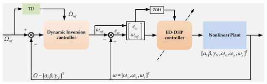
Figure 1.
Schematic of flight controller with ED-DHP.
The virtual control vector of the slow loop is designed by dynamic inversion:
where is the reference trajectory vector of the fast loop subsystem. is the acceleration vector, which can be measured by an accelerometer. is the gravity vector. and are the coordinate transformation matrix calculated by attitude angles with pitch angle , yaw angle , and roll angle , as well as attack angle and sideslip angle .
And the matrix function can be written as:
As we can see from the virtual control vector (4), the derivative of guidance commands is necessary to improve the dynamic performance of the system. To alleviate the “items of explosion” problem, the tracking differentiator was introduced [26], which is described as:
where is the guidance command, is the differential value. and are positive parameters to be designed.
3.2. The Fast Loop Error Dynamics of Attitude System and Model Identification
The dynamical equations of the fast loop can be rewritten as:
The symbols in Equation (6) are given as:
The disturbance term expressed parameter uncertainty and modeling error, which causes the inaccurate trim value and external disturbance.
The trim surface is set as , which can be roughly obtained by the newton iteration method offline, and the standard control input is given by:
where is the output vector of actor NN in ED-DHP.
Substitute Equation (7) into Equation (6) and subtract the reference trajectory dynamics , we can obtain:
And the problem can be written in a discrete form by Euler’s method:
where is known. , and reference trajectory function are unrevealed, however.
The first equation in Equation (9) can be rewritten as follows:
where
can be directly calculated from the measured vehicle attitude. is the information matrix, which is only related to the previous output vector of the actor NN. is the parameter matrix, and it can be identified in real-time by the RLS method:
where is the prediction error and is the forgetting factor. is the estimation covariance matrix.
3.3. ED-DHP Framework
For the system dynamics (9), the perfect control input contains the feedforward input and the feedback input if the system dynamics is known [27].
The symbols in Equation (14) are given as follows. Function is known as the utility and is selected based on the quadratic energy function in this paper. is defined as a performance measure function or value function in RL. It represents the sum of expected future reward from the current state. Matrices and are positive definite. is a discount factor.
For learning the control strategy of the attitude system without some prior knowledge, the augmented system is constructed in terms of and [28,29] as:
So we could have the following controller for the fast loop subsystem as follows: (Here, the second part is the output vector of actor NN, and the third is designed to compensate for the total uncertainty.)
For the augmented system (18), the cost function and value function can be rewritten as:
where
Figure 2 shows the schematic of ED-DHP. The critic NN approximates the derivatives of the value function concerning the augmented state , defined as .
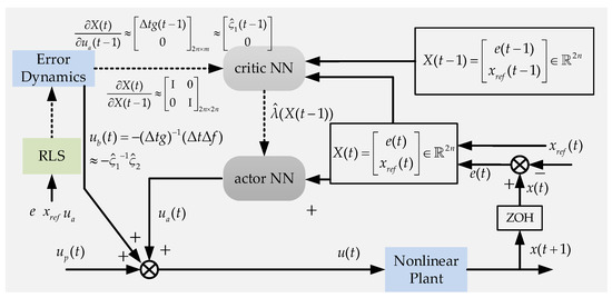
Figure 2.
Schematic of ED-DHP.
As can be observed from this figure, the previous derivatives of the value function and the augmented state are required to be stored and used in updating the NNs, without predicted ones. The control policy estimated by the actor NN is updated by minimizing the value function. A two-layer neural network with one hidden layer containing 10 neurons is used as the critic NN and actor NN in this article, shown in Figure 3. The hidden-layer activation function is tanh. For the critic NN, , and represent the weights from the ith input node to the jth hidden layer node and the jth hidden node to the kth output node, respectively. For the actor NN, , and represent the weights from the ith input node to the jth hidden layer node and the jth hidden node to the kth output node. The intermediate variables for the jth hidden layer node and the outputs of the neural networks can be written as:
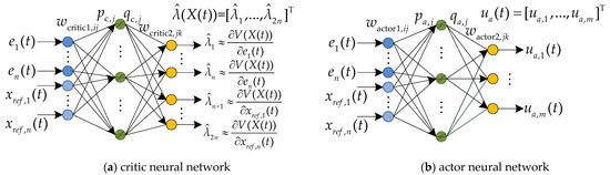
Figure 3.
The critic NN and actor NN.
It is desired to update the critic NN by minimizing the square Bellman error:
where
In Equation (30), and can be approximated by critic NN. is calculated by actor NN. The transition matrices and can be obtained from Equation (9). Because the partial derivative with respect to the angle rate of other channels is close to 0, we can obtain the transition matrices as follows: (The input dynamics are identified by RLS.)
The weights of critic NN are updated by the gradient descent method with a learning rate .
To minimize the value function in Equation (21), we can update the weights of actor NN by the gradient descent method, similarly. The learning framework of ED-DHP is shown in Algorithm 1.
| Algorithm 1 Learning Framework |
| Require: |
| Simulation parameters: sampling time and the total simulation time ; |
| The controller parameters for the slow loop subsystem; |
| The forgetting factor of RLS; |
| The positive definite matrices; |
| The discount factor and the learning rates of two neural networks. |
| Initialize: |
| The initial states and inputs of the air vehicle; |
| The parameter matrix and the estimation covariance matrix of RLS; |
| Initialize the parameters of two neural networks randomly. |
| Online Learning: |
| 1: for t = 0 to do; |
| 2: Calculate reference angular rate vector of the fast loop subsystem with (4); |
| 3: Obtain the angular rate vector through the sensors; |
| 4: Update the RLS model with (11)–(13); |
| 5: Update the parameters of the critic NN with (33) and (34); |
| 6: Update the parameters of the actor NN with (35) and (36); |
| 7: Calculate the output vector of the actor NN with (26)–(28); |
| 8: Calculate the control input vector of the air vehicle with (19); |
| 9: Get the next system states by taking action ; |
| 10: end for. |
4. Numerical Simulation and Discussion
In this section, the ED-DHP’s capability of online self-learning without complete knowledge of system dynamics and reference trajectory dynamics is demonstrated. Two numerical simulations are conducted to verify the design of the control scheme, sinusoidal signal tracking at a fixed operating point and command tracking with a morphing process at variable operating points.
4.1. Example 1
The scheme firstly controls the angle of attack , sideslip angle , and bank angle to track the sinusoidal reference signals under the condition of a fixed operating point. The initial conditions are , , and . The primary control surfaces are and , which are close to the sketchy trim values. The reference commands are designed as:
The controller parameters for the slow loop subsystem are set as . The positive parameters of TD are designed as and . The forgetting factor of RLS is , to ensure consistency of the identification. It was found that if is set to a value less than 1, the identification speed is improved with the reduction of stability of ED-DHP. So the parameters identified onlineshould have the correct sign and, to some extent, the correct relative magnitude in the self-learning process. The initial parameter matrix of RLS is set as follows, (which only conforms to the polarity of the vehicle):
The initial estimation covariance matrix is set as:
The ED-DHP is implemented with the sampling time , and the integration period of RK4 is 0.001s. The weights of the critic NN and actor NN are randomly initialized in . The positive definite matrices of ED-DHP are and . The learning rate of critic NN is and of the actor NN is , respectively. The discount factor is set as 0.99.
As is shown in Figure 4, Figure 5, Figure 6 and Figure 7, both , , and can follow the reference signals after less than 2 s. From Figure 4, we see that during the learning process, the max dynamic tracking errors of , , and are 0.6 degrees, 1 degree, and 0.8 degrees, respectively.
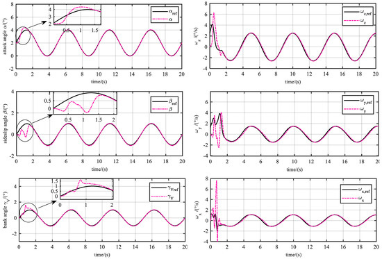
Figure 4.
Tracking performance. The attack angle, sideslip angle, and bank angle response (left), and angular rates responses (right). It can be seen that the angles can follow the reference signals in about 2 s. There are certain oscillations in each channel to fully excite the identification and optimize the learning process.
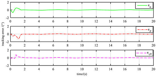
Figure 5.
Tracking errors. It takes a little longer to learn to control the sideslip angle and bank angle than the attack angle. This can be attributed to the stronger coupling characteristics between the roll and yaw channels.
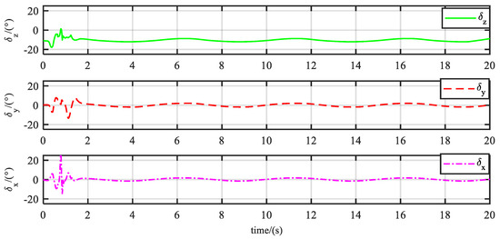
Figure 6.
Control signals. It is worth noting that the equivalent surface of the pitch channel is initialized near the rough trim value of –11 degrees. If the trim value of your plant is close to 0, you can initialize it at 0 degrees.
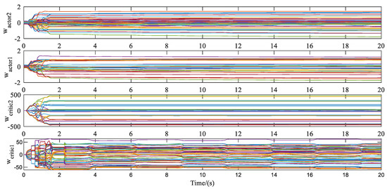
Figure 7.
Weights updating of actor NN and critic NN. The parameters of neural networks converge to a steady state at about 1.4 s.
After the parameters of the neural networks converge to a steady state, the tracking errors of the three angles are maintained within 0.05 degrees. The same observation is made from the parameters of two NNs, as illustrated in Figure 7. The ED-DHP shows good stability even though the learning rate does not change throughout the tracking process. However, it is worth noting that the angular rate loop has a large amplitude oscillation, especially the yaw rate loop and the roll rate loop. The phenomenon is mainly aroused by the cross-channel coupling and characteristics of the air vehicle’s roll channel.
4.2. Example 2
To further verify the effectiveness and robustness of the proposed control scheme, the guidance command tracking with morphing process at variable operating points is considered, as well as the model uncertainty.
The initial tracking errors of the three channels are 1 degree, and the control parameters of the fast loop and slow loop are all the same as in Section 4.1. Three cases with different parameters perturbation are carried into the numerical simulation, shown in Table 1. The switch of the air vehicle’s configuration occurs between 20 s~23 s. To ensure the stability of initial learning, TD starts to act on the system at 5 s.

Table 1.
The parameter uncertainty for 3 cases.
As is shown in Figure 8, the whole duration of the simulation is 30 s, and the guidance commands are not concrete expressions. The controller makes the vehicle track the reference value of the attack angle of 2 degrees and maintains a sideslip angle and bank angle of around 0 degrees. After that, the vehicle is lifted at an attack angle of 8 degrees, morphing and maintained at the current angle of attack. Additionally, in this simulation condition, the flight speed of the vehicle is fast, and the dynamic pressure changes dramatically within the simulation time.
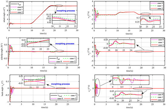
Figure 8.
Tracking performance under three cases. In case 1, the dynamic pressure and moment coefficients are larger. So the system owns stronger control efficiency, causing higher requirements for the servo.
, , and can follow the reference signals after about 2 s. In Figure 9, the max tracking errors of , , and are both within 0.5 degrees before 2 s. The tracking errors of the attack angle are shown in Table 2.
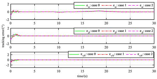
Figure 9.
Tracking errors under three cases.
Table 2.
Tracking errors of attack angle at different time periods.
Figure 10 shows that the drastic changes in control surfaces are mainly concentrated in the first two seconds of the learning phase. In the lifting process, the symbol change of the pitch channel’s equivalent control surface has occurred, which means the desperate transformation of the operating points. This can be furthermore reflected in the sharp change of critic NN parameters in Figure 11, while the parameters of actor NN are only slightly adjusted.
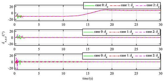
Figure 10.
Control signals under three cases.
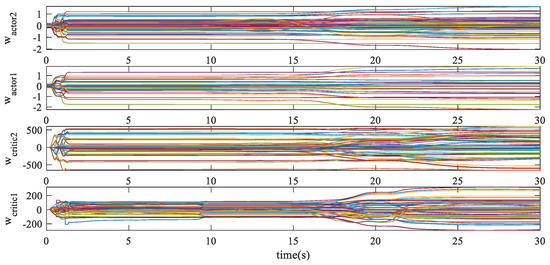
Figure 11.
Weights updating of actor NN and critic NN.
The parameters of critic NN are obviously affected during the morphing process. However, the actor NN is adjusted slightly. It shows that the updating of NNs is mainly related to the tracking error. When actor NN owns strong control ability, that is, the tracking errors are very small during the morphing, the network parameters can adapt to the process only by fine-tuning.
5. Conclusions
This article presents the ED-DHP method for online nonlinear flight attitude control. ED-DHP defines the augmented system state, which contains tracking error and reference trajectory, to solve the tracking problem. This can make the actor neural network learn the feedforward and feedback control terms simultaneously without requiring complete knowledge of the vehicle dynamics and the reference trajectory dynamics. An RLS method is used to identify not only the input dynamics but also the total uncertainty based on the error dynamics in real-time.
This proposed method is applied in two numerical experiments based on a morphing air vehicle model: sinusoidal signal tracking at a fixed operating point and guidance command tracking with morphing process at variable operating points. The results indicate the robustness and adaptiveness of ED-DHP. They also reveal that ED-DHP can learn the multichannel attitude control policy online without offline training.
In the meantime, there are some questions worth pondering:
- Augmented state increases the dimension of the system state space, which may affect the convergence speed of the algorithm without offline training;
- The systems with input constraints can be further considered by designing the new cost function to make this method better apply to real vehicle systems;
- ED-DHP is suitable for the control of fast loop subsystems. It is necessary to optimize the error dynamic and RLS method to expand the application scenarios of ED-DHP.
Author Contributions
Conceptualization, X.H. and J.L.; methodology, X.H., H.Z. and Y.P.; software, X.H.; validation, Y.Z., J.L. and Z.W. formal analysis, X.H., Y.Z. and J.L.; writing—original draft preparation, X.H.; writing—review and editing, Y.Z., J.L., H.Z., Z.W. and Y.P.; visualization, Y.Z.; supervision, J.L. and Z.W. All authors have read and agreed to the published version of the manuscript.
Funding
This research was funded by the National Natural Science Foundation of China, grant number U21B2028.
Institutional Review Board Statement
Not applicable.
Informed Consent Statement
Not applicable.
Data Availability Statement
Not applicable.
Conflicts of Interest
The authors declare no conflict of interest.
References
- Chai, R.; Tsourdos, A.; Savvaris, A. Review of advanced guidance and control algorithms for space/aerospace vehicles. Prog. Aerosp. Sci. 2021, 122, 100696. [Google Scholar] [CrossRef]
- Ding, Y.B.; Yue, X.K.; Chen, G.S. Review of control and guidance technology on hypersonic vehicle. Chin. J. Aeronaut. 2022, 35, 1–18. [Google Scholar] [CrossRef]
- Kober, J.; Peters, J. Reinforcement Learning in Robotics: A Survey. In Learning Motor Skills. Springer Tracts in Advanced Robotics; Springer: Cham, Switzerland, 2014; Volume 97, pp. 9–15. [Google Scholar]
- Degrave, J.; Felici, F.; Buchli, J. Magnetic control of tokamak plasmas through deep reinforcement learning. Nature 2022, 602, 414–419. [Google Scholar] [CrossRef] [PubMed]
- Tang, X.; Qin, Z.T.; Zhang, F. A Deep Value-network Based Approach for Multi-Driver Order Dispatching. In Proceedings of the 25th ACM SIGKDD International Conference, Anchorage, AK, USA, 4–8 August 2019; pp. 1780–1790. [Google Scholar]
- Zeng, S.; Kody, A.; Kim, Y. A Reinforcement Learning Approach to Parameter Selection for Distributed Optimization in Power Systems. Available online: https://arxiv.org/abs/2110.11991 (accessed on 22 October 2021).
- Dong, C.Y.; Liu, C.; Wang, Q. Switched Adaptive Active Disturbance Rejection Control Of Variable Structure Near Space Vehicles Based On Adaptive Dynamic Programming. Chin. J. Aeronaut. 2019, 32, 1684–1694. [Google Scholar] [CrossRef]
- Liu, C.; Dong, C.Y.; Zhou, Z.J. Barrier Lyapunov Function Based Reinforcement Learning Control For Air-Breathing Hypersonic Vehicle With Variable Geometry Inlet. Aerosp. Sci. Technol. 2019, 96, 105537. [Google Scholar] [CrossRef]
- Jia, C.H.; Gong, Q.H.; Huang, X. Synchronization Control of Nonlinear Chaotic Systems with Deep Reinforcement Learning Algorithm. In Proceedings of the International Conference on Guidance, Navigation and Control, Tianjin, China, 23–25 October 2020; pp. 1673–1682. [Google Scholar]
- Hui, J.P.; Wang, R.; Yu, Q.D. Generating new quality flight corridor for reentry aircraft based on reinforcement learning. Acta Aeronaut. Astronaut. Sin. 2022, 43, 325960. [Google Scholar]
- Kiumarsi, B.; Vamvoudakis, K.G.; Modares, H. Optimal and Autonomous Control Using Reinforcement Learning: A Survey. IEEE T. Neur. Net. Lear. 2018, 29, 2042–2062. [Google Scholar] [CrossRef]
- Ferrari, S.; Stengel, R. Online adaptive critic flight control. J. Guid. Control. Dynam. 2004, 27, 777–786. [Google Scholar] [CrossRef]
- Mu, C.X.; Ni, Z.; Sun, C.Y. Air-breathing hypersonic vehicle tracking control based on adaptive dynamic programming. IEEE T. Neur. Net. Lear. 2017, 28, 584–598. [Google Scholar] [CrossRef] [PubMed]
- Xia, R.; Chen, M.; Wu, Q. Neural Network based Integral Sliding Mode Optimal Flight Control of Near Space Hypersonic Vehicle. Neurocomputing 2020, 379, 41–52. [Google Scholar] [CrossRef]
- Huang, Y.; Liu, D. Neural-network-based optimal tracking control scheme for a class of unknown discrete-time nonlinear systems using iterative ADP algorithm. Neurocomputing 2014, 125, 46–56. [Google Scholar] [CrossRef]
- Wang, Q.; Gong, L.G.; Dong, C.Y. Morphing aircraft control based on switched nonlinear systems and adaptive dynamic programming. Aerosp. Sci. Technol. 2019, 93, 105325. [Google Scholar] [CrossRef]
- Han, X.; Zheng, Z.; Liu, L. Online policy iteration ADP-based attitude-tracking control for hypersonic vehicles. Aerosp. Sci. Technol. 2020, 106, 106233. [Google Scholar] [CrossRef]
- Bertsekas, D.P.; Homer, M.L.; Logan, D.A. Missile Defense and Interceptor Allocation By Neuro-Dynamic Programming. T-SMCA 2000, 1, 42–51. [Google Scholar] [CrossRef]
- Van Kampen, E.; Chu, Q.P.; Mulder, J.A. Continuous Adaptive Critic Flight Control Aided with Approximated Plant Dynamics. In Proceedings of the AIAA Guidance, Navigation, and Control Conference and Exhibit, Keystone, CO, USA, 21–24 August 2006. [Google Scholar]
- Zhou, Y.; van Kampen, E.J.; Qi, P.C. Nonlinear Adaptive Flight Control Using Incremental Approximate Dynamic Programming and Output Feedback. J. Guid Control. Dynam. 2016, 40, 1–8. [Google Scholar] [CrossRef]
- Zhou, Y.; van Kampen, E.J.; Qi, P.C. Incremental model based online dual heuristic programming for nonlinear adaptive control. Control. Eng.Pract. 2018, 73, 13–25. [Google Scholar] [CrossRef]
- Li, H.X.; Sun, L.G.; Tan, W.Q. Switching Flight Control for Incremental Model-Based Dual Heuristic Dynamic Programming. J. Guid, Control. Dynam. 2020, 43, 1–7. [Google Scholar] [CrossRef]
- Liu, J.H.; Shan, J.Y.; Rong, J.L. Incremental reinforcement learning flight control with adaptive learning rate. J. Astronaut. 2022, 43, 111–121. [Google Scholar]
- Lee, J.H.; van Kampen, E.J. Online reinforcement learning for fixed-wing aircraft longitudinal control. In Proceedings of the AIAA Scitech 2021 Forum, Online, 11–15 January 2021. [Google Scholar]
- Heyer, S.; Kroezen, D.; Van Kampen, E. Online Adaptive Incremental Reinforcement Learning Flight Control for a CS-25 Class Aircraft. In Proceedings of the AIAA Scitech 2020 Forum, Orlando, FL, USA, 6–10 January 2020. [Google Scholar]
- Han, J.Q. Auto Disturbance Rejection Control Technology; National Defense Industry Press: Beijing, China, 2008; pp. 64–67. [Google Scholar]
- Lewis, F.L.; Vrabie, D. Reinforcement learning and adaptive dynamic programming for feedback control. IEEE Circ. Syst. Mag. 2009, 9, 32–50. [Google Scholar] [CrossRef]
- Kiumarsi, B.; Lewis, F.L. Actor-critic-based optimal tracking for partially unknown nonlinear discrete-time systems. IEEE Trans. Neural Netw. Learn. Syst. 2015, 26, 140–151. [Google Scholar] [CrossRef]
- Modares, H.; Lewis, F.L. Optimal tracking control of nonlinear partially-unknown constrained-input systems using integral reinforcement learning. Automatic 2014, 50, 1780–1792. [Google Scholar] [CrossRef]


Disclaimer/Publisher’s Note: The statements, opinions and data contained in all publications are solely those of the individual author(s) and contributor(s) and not of MDPI and/or the editor(s). MDPI and/or the editor(s) disclaim responsibility for any injury to people or property resulting from any ideas, methods, instructions or products referred to in the content. |
© 2022 by the authors. Licensee MDPI, Basel, Switzerland. This article is an open access article distributed under the terms and conditions of the Creative Commons Attribution (CC BY) license (https://creativecommons.org/licenses/by/4.0/).