1. Introduction
The mathematical modeling of three-phase electrical systems to evaluate electromagnetic transients in the different equipment and devices that are part of these systems is determined by high-order, nonlinear and time-varying models and generally complicated systems.
The mathematical model for an electrical power system using field approaches was developed in [
1]; here, the model of the transmission lines are obtained by partial differential equations and the equation of the supply to the transmission line uses two first-order differential equations. The real-time simulation of a transmission line with the objective of knowing the behavior of harmonic signals in line transients is presented in [
2], and the dynamic domain is also applied to the transmission line, which allows the visualization of the steady state and the transient condition. Different configurations of power transmission lines are simulated in [
3], however, here, a negative capacitance is added in parallel with the inductance in the
equivalent circuit that allows one to improve the simulation of transmission lines. The study of the available transfer capability in a transmission system to know the transient stability is proposed in [
4], performing network analysis with ultra-high-voltage lines. The stability control in long transmission lines can incorrectly operate the equipment, which is simulated and analyzed in [
5]. A three-phase power transformer is modeled and simulated with a digital implementation in [
6], and the transformer model is verified with experiments carried out on a 6 kVA transformer.
Recently, with the supply of electrical energy from renewable energy sources such as wind turbines and photovoltaic panels, electrical system modeling includes elements and equipment that these new electrical power generation systems require. In [
7], the modeling and simulation of a photovoltaic power system is proposed that is connected to the network with a three-phase power of 8kW for at home purposes with a PQ controller. The modeling of a wind turbine for harmonic analysis with different switching techniques is proposed in [
8] where doubly-fed induction generators are connected to the back-to-back power converter. The modeling and simulation of a photovoltaic system using Matlab with the aim of considering the irradiance and analyzing the power quality was found in [
9]; in addition, the behavior of a three-phase system with different inverter control techniques is described when the PV system is generating energy. Likewise, the simulation of a distributed generation model with the use of multi-energy sources for three-phase stability studies was developed in [
10], wherein a unified interface model for a synchronous generator and inverter that applies to different types of energy—electric, heat and hydrogen—was proposed.
The difficulty in the modeling, analysis and control of three-phase electrical systems has become one of the reasons for the use of various software such as in [
9], wherein Matlab software is used. The application of the Multisim software in the simulation of three-phase electrical circuits was found in [
11]. Furthermore, the study of electromagnetic transients in three-phase electrical systems for transmission and distribution models using the EMTP software was proposed in [
12].
Other interesting references with the application of coordinate transformations applied to electrical systems are the following: the comparison of current regulators in three-phase electrical systems in the reference frames: (1) natural
, (2) orthogonal stationary
and (3) orthogonal stationary
were presented in [
13]. A new reference frame, called a reduced reference frame, which can be used for unbalanced three-phase systems, was proposed in [
14]. The properties of three transients with unbalanced sources were investigated in [
15], where the Clarke and Park transformations are used. The energy management architecture model using a complete supervisory control and data acquisition system in a educational building was presented in [
16]. An energy management system applied to isolated micro grids was proposed in [
17], wherein they apply a PID controller which contains coordinate transformations from
to
.
When considering a renewable power system and its control, full modeling can be challenging because the system will have different energy domains. For example, if the system is the interconnection of thermoelectric, hydroelectric, wind turbines and photovoltaic panels as sources of generation, their transmission and distribution to electrical loads, then there are electrical, mechanical, thermal and hydraulic subsystems, subsystems for control as well as three-phase systems, due to which factors the bond graph is a system modeling methodology that can be applied to the systems formed by different energy domains. Likewise, the analysis and control of systems in the bond graph are direct and physically achievable. In addition, the modeling of systems with multiple phases or axes has been solved with multibond graphs which are vector bond graphs.
The bond graph theory is based on an approach to modeling power transfer through ports called bonds. In this way, a structured approach to modeling dynamic systems is presented in the bond graph.
The main characteristics of the bond graph can be stated below: (1) The bond graph allows the modeling of systems formed by different energy domains (electrical, mechanical, hydraulic, thermal, magnetic); (2) Through the causal information, the relationship between the elements of a system is known, determining mathematical models in transfer function or in state space, likewise, structural properties such as stability, controllability and observability can be directly obtained in the bond graph model without requiring its mathematical model; (3) Linear and nonlinear, invariant and time-varying systems with lumped distributed parameters can be modeled in a bond graph; and (4) Controllers can be designed in a bond graph environment.
The modeling of robots, cars, projectiles or multi-axis systems often leads to complicated mathematical models. Even in bond graphs, these systems can result in models that cannot easily apply the methodology and its applications in the physical domain. Thus, the introduction of multibond graphs as an extension of bond graphs turns out to be a natural way to model multibody systems.
In modeling with multibond graphs, single bonds are grouped into multibonds. Likewise, the generalized power variables of effort and flow in bond graphs are now vectors of effort and flow in multibond graphs whose matrix product determines power.
Some papers on fundamentals and application with multibond graphs have been published, some of which are cited below: the basic concepts in the modeling with multibond graphs of physical systems are proposed in [
18]. The causality assignment in vector bond graphs is introduced in [
19]. The modeling of mechanical systems with multibond graphs was developed in [
20]. The decomposition of multibody elements such as resistors, inertias, capacitors, transformers and gyrators into their equivalent in junctions, bonds and 1-port and 2-port elements was presented in [
21].
Recently, some developments with multibond graphs have been published, and the representation of electrical circuits of phasors containing real and imaginary parts with two-dimensional multibond and steady state was proposed in [
22]. The linearization of a class of nonlinear systems that can be modeled with multibond graphs was presented in [
23]. The direct determination of the steady-state response for LTI systems modeled with multibond graphs with a derivative causality assignment to the storage elements was proposed in [
24].
In this paper, the modeling of three-phase electrical systems in coordinates is presented. The modeling of an electrical system in coordinates determines the systems of time-varying differential equations, and by applying Park’s transformation, an equivalent time-invariant system is obtained. In the analysis of electromagnetic transients to electrical systems in the coordinates , the differential equations are determined with inductive and capacitive elements as well as the connectivity with the different elements, whilst ascertaining whether the three phases are balanced is difficult and complicated.
Electrical system simulation software allows graphic results to be obtained, but the structural mathematical analysis of the system is generally not its objective. Thus, this paper enables the modeling of model-balanced or -unbalanced three-phase electrical systems in the multibond graphs environment.
Bond graph tools can be applied in multibond graphs. In particular, a lemma to directly obtain the multibond graph in the coordinates is proposed and from this, other lemma to determine the mathematical model in state space is presented. Therefore, the advantages of this paper with respect to traditional developments were exposed.
The works developed in bond graphs [
25,
26,
27] that mainly use the Park transformation for the modeling of electrical machines are bond graphs built from the mathematical model in the state space of the system and it is effectively verified that the bond graph is correct. However, general methodologies similar to this proposed paper are not reported. In multibond graphs, practically no papers have been published on the modeling of three-phase electrical systems, and as such, this paper is an interesting proposal on the modeling of three-phase electrical systems in coordinates
and its transformation in coordinates
.
Therefore, the primary advantages of this paper are the modeling of three-phase electrical systems in coordinates in a direct way, directly obtaining its symbolic representation in state space and its derivation of the model in coordinates .
Section 2 describes the traditional modeling of a power system from coordinates
to coordinates
. The essential elements in modeling systems with multibond graphs are developed in
Section 3. In this section, the junction structure and state space of a system modeled in multibond graphs are presented. In
Section 4, a lemma and procedure for directly obtaining the multibond graph of an electrical system are proposed. Two examples applying the described methodology are solved, including the simulation results. In
Section 6, describes the aplication of the metodology. Finally,
Section 7 gives the conclusions.
2. Problem Statement
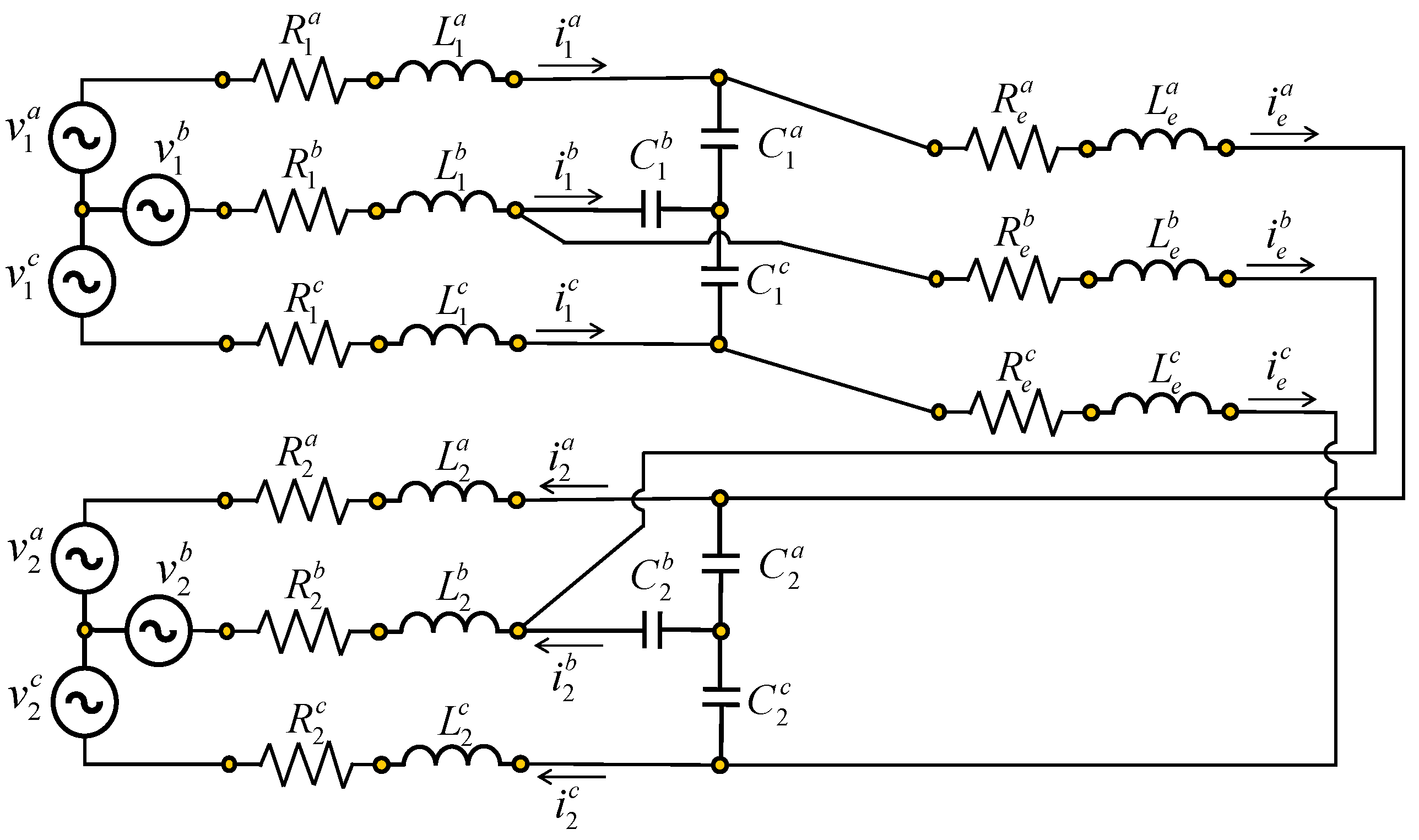
Most commercial electrical power is generated in three-phase systems [
28,
29]. Consider a simple three-phase circuit formed by two generators and a line transmission which is shown in
Figure 1 [
30].
With the objective of obtaining the dynamic equations of the system for the analysis of electromagnetic transients, then applying the voltages law to the circuit of
Figure 1 gives
where
and
denote the three-phase voltages of supply sources 1 and 2, respectively;
and
denote the three-phase voltages across the resistors
,
and
respectively;
and
denote the three-phase voltages across the inductances
,
and
respectively;
and
denotes the three-phase voltages across the capacitances
and
, respectively.
The relationships between the resistors and inductors are
where
and
are the voltages in each phase
of supply sources 1 and 2, respectively;
and
are the voltages in each phase
of capacitors 1 and 2, respectively.
where
and
are the voltages and currents in each phase
of resistor 1, respectively;
and
are the voltages and currents in each phase
of inductance 1, respectively;
is the resistance matrix 1 of the three phases
,
and
are the resistors 1 in each phase
, respectively, and
is the inductance matrix 1 of the three phases
,
and
denote the inductance 1 in each phase
, respectively.
In the same form, it is established that
where
and
denote the three-phase voltages and currents in
, respectively;
and
denote the three-phase voltages and currents in
, respectively; and
and
denote the three-phase voltages in
and
, respectively.
and
are the resistance matrices of
e and 2 of the three phases
, respectively, and
and
are the inductance matrices of
e and 2 of the three phases
, respectively.
The relationships for the capacitors are
where
and
are the three-phase currents and voltages in
, respectively;
and
are the three-phase currents and voltages in
, respectively,
and
are the capacitance matrices 1 and 2 of the three phases
respectively, and
,
and
are the capacitors 1 in each phase
By substituting from (
4) and (
9) into (
1), (
2) and (
3)
in addition,
and
, and the equations for the capacitors are
From (
12) to (
16) represent a fifteenth-order dynamic system for a simple three-phase circuit. However,
and
are three-phase voltage sources, these sources are typically balanced and given by
where
is the maximum value of
v and
w is the angular frequency such that
being
f the frequency in
.
Hence, considering (
17) with (
12) to (
16), the dynamic system is a linear time-varying (LTV) system of 15 dimensions.
A great simplification in the mathematical description of a three-phase electrical system is obtained from Park’s transformation. The effect of Park’s transformation is simply to transform all stator quantities from phases
a,
b and
c into new variables, the frame of reference of which moves with the rotor [
28,
29,
31]. Electrical systems that have three-phase voltages and currents are complicated to model, analyze and control to determine time-varying systems, so the Park transformation has been applied, which allows obtaining equivalent systems without dependence on time.
In order to remove the time dependence, Park’s transformation can be used. This transformation for voltages is defined by
where
the angle between the
d axis and the rotor is given by
where
w is the rated angular frequency in
.
Park’s transformations for currents and flux linkages are expressed by
Now, representing (
12), (
13) and (
14) by Park’s transformation,
and from (
15) and (
16), the equations for the capacitors are
in terms of
where
under balanced conditions
it is well known that
is given by
substituting (
38) into (
27), (
28) and (
29)
a ninth-order LTI dynamic system for the inductances is obtained.
Now, substituting (
38) into (
30) and (
31)
The complete system in terms
is defined by (
39), (
40), (
41), (
42) and (
43) representing a 15th order LTI system.
3. Modeling in Multibond Graphs
In the connection of two elements, components or systems, there is always a power transfer
. This power in generalized terms described in bond graph modeling is defined as the product of effort
and flow
. Likewise, the power link is represented by a power bond that is illustrated in
Figure 2 [
32].
Bond graph modeling can be applied to systems of different energy domains, that is, to electrical, mechanical, hydraulic, and thermodynamic systems. The generalized variables for these different systems are indicated in
Table 1.
In bond graph modeling, two additional variables are required to characterize a system, in which variables are called energy variables which are momentum and displacement . The time integral of an effort defines a momentum: and the displacement is the time integral of a flow: .
One of the fundamental properties in bond graph models is the causality that is applied to each of the elements that constitute part of a model. With the application of the causal stroke, each bond accurately indicates the input and output signals, as illustrated in
Figure 3, which is a power bond with its causality [
32].
According to the type of element, it has a given causality, as shown in
Table 2.
Many systems can generally be modeled as multiport power elements. For example, mechatronic systems that are constructed of mechanical, electrical and hydraulic subsystems but in turn have movements in three axes
; electrical power systems can be represented as systems with multiport phases
, likewise, hydraulic and thermal systems with a multiport can be modeled. Therefore, systems modeled with bond graphs can be represented with multibond graph models with the advantages of structural modeling, analysis and control that determine bond graphs which are generalized and extended with multibond graphs [
18,
20].
Firstly, the notation of the variables generalized with multibond graphs are efforts
and flows
with an underscore indicating that these variables determine vector bond notation, which is a composition of three bonds corresponding to the three perpendicular axes in a multibond graph.
Figure 4 shows a multibond and its equivalent in bonds [
18,
20].
Modeling with multibond graphs is common for the application to vectors with three elements for physical systems, but this does not limit the fact that it can be extended to higher-order vectors [
18]. The power in a multibond is defined by
where
is the transpose of the column vector
and
A general multibond graph indicating the generalized variables in each multibond and the junctions or multiport elements
is shown in
Figure 5 [
18].
The essential elements in modeling with multibond graphs are described in
Appendix A.
The link of the different elements that are part of a system can be organized into fields as illustrated in
Figure 6. Considering a model in a multibond graph with a predefined integral causality assignment, its fields and the key vectors.
Figure 6 presents the causal relationships between these elements that describe the system.
The different multiport fields in a multibond graph that are shown in
Figure 6 determine:
System input is the power supply through the source multiport field denoted by .
The power exchange due to the connection in multiport junctions or or in multiport transformers are carried out in the multiport junction structure.
Storage elements and determine the energy storage multiport field denoted by that they are associated with the energy variables and , variables which derive in the following state variables:
- -
When the storage elements have integral causality, they determine the linearly independent state variables with the co-energy vector .
- -
When the storage elements have derivative causality, they determine the linearly dependent state variables with the co-energy vector .
The key vectors and establish the relation between the energy dissipation multiport field denoted by and the multiport junction structure through the mixture of power variables and .
are the system outputs that are obtained from the multiport junction structure to the detectors and are denoted by .
The mathematical model of a system based on a multibond graph is determined following Lemma 1.
Lemma 1. Consider a multibond graph model with a predefined integral causality assignment that represents a system whose block diagrams is shown in Figure 6 and the multiport junction structure is defined bywhere the entries of are in the set and determines the transformer module which are constants or co-energy functions and the constitutive relations for the multiport elements arethen, a state variable representation in terms of co-energy is defined bywherewith Proof. From the second and third lines of (
47) with (
50) and (
51)
The solution of (
73) and (
74) can be expressed by
with
and
with
from the fifth line of (
47) with (
48) and (
49) and deriving
by substituting (
75) and (
77) into the first line (
47) with (
50) and (
51)
if we expressed
and
(
80) can be reduced as
and substituting (
79) into (
81) with (
54) to (
62), the space state representation defined by (
52) is proven. □
For the output, from the fourth line of (
47) with (
50) and (
51)
substituting (
75) and (
77) into (
82),
with (
63) and (
64), (
83) can be expressed by
from (
84), (
57) and (
58) with (
59) to (
62), the output equation (
53) is proven.
Note that the multibond graph model permits the representation of systems with integral and derivative causality assignments.
In the next section, a procedure to represent electrical power systems in a multibond graph approach is proposed.
5. Study Cases
1. A basic electrical power system is illustrated in
Figure 15. It is built by two three-phase sources linked by a transmission line that is a resistance in series with an inductance.
Applying the modeling methodology with multibond graphs of systems and Lemma 2, the three-phase system in coordinates
is shown in
Figure 16.
Inside the dotted box, we have the multibond graph in coordinates , and on the outside, we have the supply voltages and the current of the system in coordinates connected through multiport transformers modulated by the Park’s transformation matrix. The multibond graph model inside the blue dotted line is a time-invariant model formed by the three-phase series connection of the two power supplies and , the three-phase resistance and the inductance that must be connected to a multiport gyrator.
The key vectors of the multibond graph are expressed by
the constitutive relationships of the multiport fields are given by
where the inductances and resistors is for a balanced system
The multiport junction structure of the multibond graph model is defined by
Because there are no elements in derivative causality
. In addition, from (
106)
with (
63), (
64), (
65) and (
66),
From (
103) to (
105) with (
106), the state space of this system in coordinates
is given by
A developed representation of (
111) can be expressed as
The simulation results shown in this section are based on the 20-Sim software. This software allows the modeling, analysis and simulating systems represented in bond graphs and multibond graphs in a simple and direct way.
For this case study, the system parameters are balanced three-phase voltages
and
of magnitudes of 200 V and 100 V, respectively; the balanced link impedance of these two voltage sources are with inductances
H and resistances
. The behavior of the currents in coordinates
is shown in
Figure 17.
Electrical currents in coordinates
are shown in
Figure 18. It can be noted that the electrical currents in both coordinates are stable after the end of the transient period. The transfer of coordinates
to
consists of the use of a modulated transformer with the Park transformation matrix which, in multibond graph, is simple and direct.
The transient response in coordinates is illustrated in a clear and evident way due to its characteristic invariance in time, unlike the transient response in coordinates that could have relative confusion due to the time variance for balanced systems.
This basic electrical power system can be analyzed under unbalanced conditions for the impedance of the line linking the two supply voltage sources; in this way, the new parameters are given by
The behaviors of the current in coordinates
and
are illustrated in
Figure 19 and
Figure 20, showing the flexibility of multibond graphs for modeling and simulating systems in one coordinate or another under balanced or unbalanced conditions.
2. A second case study in the modeling of three-phase electrical systems is the one shown in
Figure 1 whose multibond graph is illustrated in
Figure 21.
The elements of the multibond graph that are inside the dotted box are defined in coordinates and those that are outside are the elements in coordinates that are the supply voltages and the current measurement. Within the blue dotted line, we have the multibond graph model composed of the source connected in series with the three-phase inductance , the three-phase resistance and the multiport gyrator; the same is true for branch 2 and for the central branch e in which it is not connected to any source but to the three-phase capacitors and .
The key vectors of the multibond graph for the multiport storage elements are
for the multiport resistors
and for the multiport gyrators and the multiport sources
The constitutive relationships are given by
being
The corresponding multiport junction structure is defined by
For this example, the matrices and then and , also, and then and .
From (
112) to (
116) with (
54) and (
55), the state space model of the system is given by
It can be seen that there is a great advantage to modeling the system with multibond graphs through which the mathematical model is obtained in a compact way. In order to show the effectiveness of the proposed methodology, the simulation results of this system are obtained using the following numerical parameters: balanced three-phase voltages and of magnitudes of 200 V and 100 V, respectively; inductors H, H, H; capacitors F, F and resistors , and .
Figure 22 illustrates the behavior of the current in the coordinates
on the first branch of the resistors
and inductors
. The graphs indicate the behavior of the currents
and
with respect to time. In this case, the magnitude of the current is due to the voltage
and the impedance formed by
and
, and the capacitor
.
The currents in coordinates
of the second branch of the elements
and
are shown in
Figure 23, and the currents
,
and
with respect to time are shown.
The current in coordinates
that links the capacitors is shown in
Figure 24, and the currents
,
and
with respect to time are shown. Furthermore, the magnitude depends on the sources of supply and the capacitances
and
. It can be seen that the currents are stable. The behavior of the capacitor voltages
,
and
with respect to time are shown in
Figure 25 and
Figure 26.
The response in the voltage of indicates that the transient period could represent an unbalanced system; however, in the steady-state period, the response determines a balanced system.
Note that the multibond graph methodology for the modeling and simulation of three-phase electrical systems is presented. Likewise, the application of power electronics to control these systems can be an interesting challenge to extend the results of this paper. Recently, renewable energy sources due to their characteristics require control, and power electronics allows linking this to have control of three-phase systems; as such, this paper can be the beginning of solving this type of control problems.


 ,
, 


