Graded Evaluation of Health Status of Hydraulic System with Variable Operating Conditions Based on Parameter Identification

Abstract

In industrial production, the effective and reliable performance of hydraulic systems is closely associated with product quality, personal safety, economic efficiency, etc. It is of utmost significance to perform the health status evaluation of systems. In this paper, a least-squares recursive parameter identification algorithm is proposed to realize the graded evaluation of the health status of the hydraulic system under variable operating conditions. First, a nonlinear model of the hydraulic system is established based on a mechanism analysis. Based on the system identifiable model obtained by parameter linearization, the least squares recursive algorithm is used to get the system parameters. Second, the system measurable data are graded and labeled under the same operating condition, and the variable parameter ranges under different health states are obtained by the parameter identification algorithm. Finally, under variable operating conditions, the estimates of variable parameters are compared with the range of health state parameters to complete the system health state graded evaluation. The feasibility of the proposed evaluation method is verified by MATLAB simulation software.

1. Introduction

Hydraulic systems are widely used in industrial production, transportation, weaponry and equipment manufacturing, etc., and play an important role in equipment driving, transmission and control with the advantages of large power quality, smooth movement, long service life, easy realization of automatic control, etc. [1,2,3]. In industrial production, whether the hydraulic equipment has effective and reliable performance is directly related to the quality of products, personal safety, economic benefits, etc. At the same time, on account of the complicated and variable operating conditions, and the relatively rough operating circumstance, the rate of system deterioration and the probability of fault substantially increase. Therefore, it is extremely valuable to perform the health status evaluation of the equipment in a timely and effective manner at the early stage of degradation, and to formulate a reasonable maintenance plan and repair program [4,5].

Currently, health state evaluation methods can be generally classified into three major categories: the model-based evaluation method, the signal processing-based evaluation method and the knowledge-based evaluation method [6].

The model-based method consists in evaluating the health status of the equipment by establishing an accurate physical and mathematical model. Theoretical modeling is combined with parameter identification or state estimation by establishing a nominal model based on the structure and theory of the system [7,8]. The residuals are then obtained by comparing the estimates of the actual model parameters with the values of the theoretical model parameters, or by comparing the output of the real system with a measurable variable obtained by reconstructing the state of the system. The main approaches of the model-based method are physical model, (extended) Kalman filter, state observer, system identification, etc. [9,10]. The key to such approaches is residual generation and residual evaluation. To evaluate the system performance, ref. [11] proposed a method based on the residuals obtained from a radial basis function (RBF) fault observer, and then self-organizing mapping (SOM) and Gaussian mixture model (GMM) are applied to evaluate the health status of the hydraulic servo system based on the residuals. In order to perform the health evaluation with variable operating conditions, ref. [12] proposed a method based on health baseline and Mahalanobis distance for hydraulic systems. An observer based on a generalized regression neural network (GRNN) is established to construct a health baseline using the health state data, and the observer is used to obtain the residuals. The Marxist distance between the health baseline and the residuals is calculated and normalized to the health degree, so as to realize the variable working condition health evaluation. To implement the health state evaluation for hydraulic systems, ref. [13] proposed a residual-vector-based method, constructing an analytical model and a state observation model to obtain the residual, and using the feature of the residual vector to perform health state evaluation. In general, the challenge of the model-based method is how to establish accurate mathematical models under the problem of uncertainty in model parameters, uncertainty in nonlinear relationships and uncertainty of the resulting model with system dynamics [14,15].

The signal processing-based evaluation method uses the physical characteristics of various output signals form the monitored equipment to analyze the health status of the equipment. Commonly used methods include Fourier transform, wavelet transform, spectrum analysis and information fusion. The key to such methods is feature extraction and threshold setting (how to distinguish among health state types) [16,17]. The fuzzy synthetic evaluation model is a method used to achieve quantitative evaluation based on the affiliation theory. Duan et al. established a fault hierarchy model for the data characteristics of a hydraulic system, and evaluated the health status through data mining and the fuzzy synthetic evaluation model [18]. The gray clustering method is a way to divide the indexes into different gray classes by a gray whitening weight function. Lin [19] and Qi [20] et al. determined the weights of each evaluation index of each component of the aircraft hydraulic system by expert experience, the entropy weight method and an extension of the analytic hierarchy process, and used the gray clustering method to evaluate the weights to obtain the health status level of each component and the whole system. To obtain sensitive feature quantities for health state evaluation, ref. [21] used wavelet packet decomposition and used the magnitude of the sensitive quantities to complete the hydraulic system health state evaluation. To overcome the effect of noise on data analysis, ref. [22] proposed a method of wavelet energy transfer rate to monitor the unit gearbox health status. Taken together, the signal processing-based evaluation method requires establishing a very accurate database of signal features or setting thresholds to classify data labels.

The knowledge-based health evaluation method is an idea and method that makes full use of the experience and knowledge of experts to simulate problem solving by domain experts [23]. No mathematical model of the object under consideration is required for this method, so it is suitable for dealing with complex and large nonlinear systems. The main methods are expert systems based on knowledge, knowledge-based evolutionary methods such as artificial neural networks and Bayesian networks based on statistical knowledge, etc. The key to this type of method is network training and classification decisions [24,25]. Based on the standard LeNet, an improved convolutional neural network (CNN) with a particle swarm optimization algorithm was constructed in ref. [26], where the model was used to train the acoustic signal of the hydraulic piston pump to analyze the health status. To tackle the difficulty of severe class imbalance in faulty samples, ref. [27] proposed the invariant temporal-spatial attention fusion network (ITSA-FN) to evaluate the bearing health status with imbalance conditions. In order to rapidly predict the important performance indicators of mechanical devices, ref. [28] proposed a prediction algorithm of comprehensively using a composite variable wavelet transform, deep auto-encoder and long short term memory (CWD-LSTM) hybrid neural network. In particular, it has a great advantage for time series. To implement the medical device health status evaluation, ref. [29] proposed a partial least squares regression (PLSR) algorithm combined with deep neural networks (DNNs). Briefly, the knowledge-based method involves massive amounts of data for network training. In addition, there is high accuracy with more different kinds of data, but it cannot explain the connection between the data and the system, i.e., the conclusion has uncertainty.

Integrating the current state of the research, model-based methods have a deep theoretical foundation and strong implementability, and will remain the main direction of research in the field of health state evaluation technology in future development. Among them, the parameter estimation method is very suitable for hydraulic systems with strong nonlinearity. In this paper, the system variable parameters are used as indicators to evaluation the real health status of the system, and the system parameters are obtained by establishing a nonlinear mathematical model of the hydraulic system based on system identification. The simulation experiment was conducted using MATLAB simulation software. The fourth-order Runge–Kutta method was used to obtain the measurable data of the system, and the differential data of measurable data were obtained by a tracking-differentiator (T-D). The least squares recursive algorithm was used to identify the system parameters and obtain the health state range of the variable parameters of the system under the same operating conditions. Then, under variable operating conditions, the identification algorithm was used to obtain variable parameters and compare them with the parameter range of health state to achieve hydraulic system health state evaluation.

The main contributions and innovations of this paper can be summarized as follows:

• The idea of evaluating the health state of a hydraulic system based on parameter estimation is introduced and implemented. The simulation results verify the feasibility of this idea.
• A hydraulic system parameter identification model is given, and the parameter indicators for evaluating the health status of the hydraulic system are delineated.
• The combination of a signal processing-based method and a model-based method is performed, and the problem of evaluating the health status under variable operating conditions is solved based on the data analysis of the same operating condition.

The remaining parts of this paper are arranged as follows. Section 2 establishes a nonlinear mathematical model of the electro-hydraulic servo system for a valve-controlled cylinder system. Section 3 gives the system parameters based on the least squares recursive algorithm through the simulation experiment. Section 4 gives a specific process of evaluating the health status of the hydraulic system under variable operating conditions through the simulation experiment. Section 5 is a brief summary of this paper, together with the future research work.

2. Modeling of Electro-Hydraulic Servo System for Valve-Controlled Cylinder

In this section, a brief introduction of the electro-hydraulic position servo system is given, and a nonlinear mathematical model of this system satisfying certain conditions is established through the mechanism analysis.

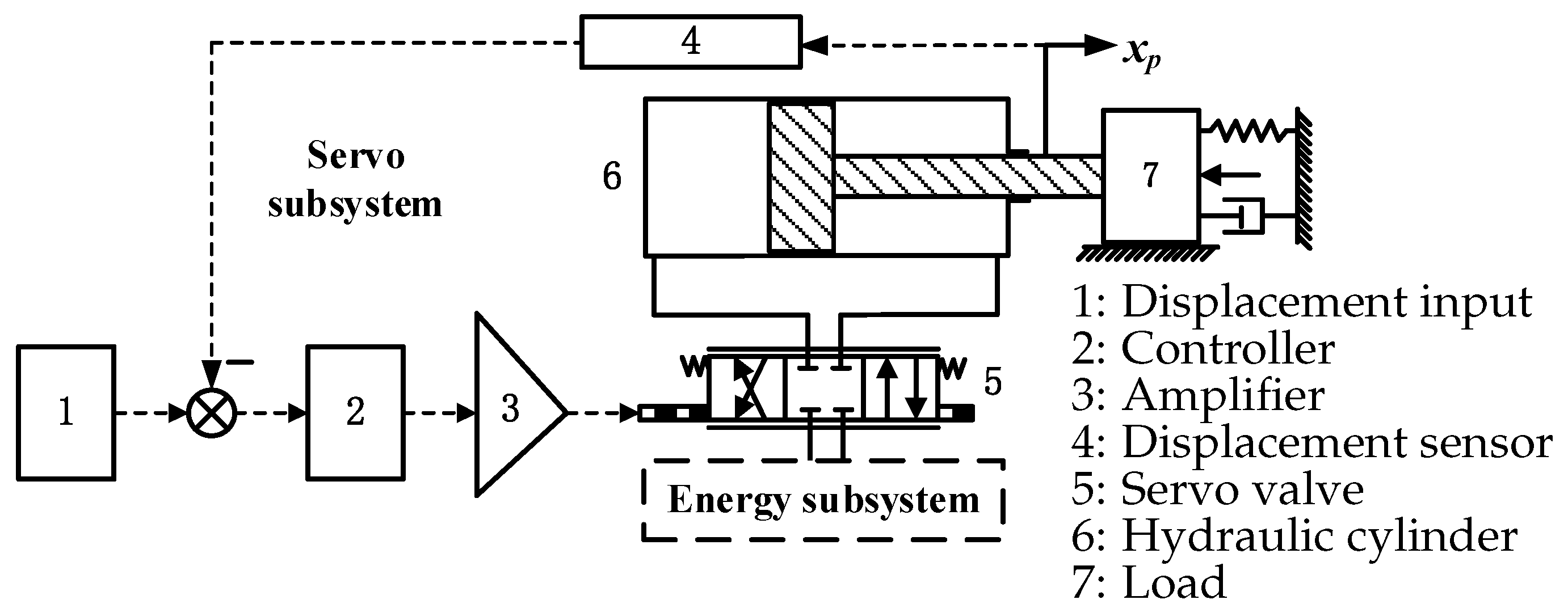
2.1. Introduction of Electro-Hydraulic Servo Position System

Hydraulic systems can be divided into two main categories: one is hydraulic transmission systems, and the other is hydraulic control systems [30]. Hydraulic transmission systems are mainly used to transmit power, and to transmit information as a supplement. The basic task is driving and speed regulation. Hydraulic control systems are mainly used to transmit information, and to transmit power as a supplement. The main task is to enable the controlled quantity to automatically, stably, quickly and accurately track the input command changes. This paper focuses on the hydraulic automatic gauge control (AGC) system for rolling mills whose main application is the electro-hydraulic position servo system, which is a hydraulic control system with servo components as the control core. The electro-hydraulic position servo system is the main application of AGC, and it has two major subsystems: energy subsystems and servo subsystems [31]. The customary term electro-hydraulic position servo system mainly denotes servo subsystems, which are generally composed of a displacement sensor and input command, controller, servo valve, hydraulic cylinder, load and other components, and its configuration is shown in Figure 1.

A system of a four-way slide valve-controlled asymmetric cylinder is shown in Figure 2. We assume that the valve is matched symmetrically, the flow at the valve port is turbulent, the supply pressure is constant, and the temperature and density are constant; the dynamics and losses of the pipeline are not considered. At the same time, considering the nonlinearity of flow-pressure at the servo valve port, the nonlinearity of the saturation characteristics of the servo valve, the nonlinearity of the internal leakage of the hydraulic cylinder and the time-varying characteristics of the liquid volume of the two chambers, as well as the nonlinearity of the friction characteristics, the mathematical model of the system is established as follows [32,33,34,35,36].

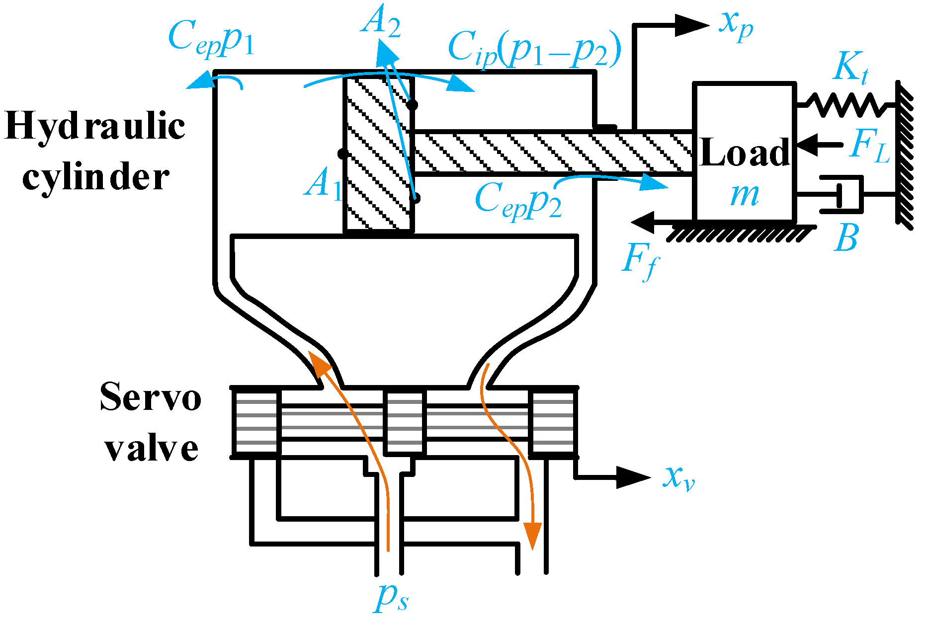
2.2. System Modeling

Servo valve dynamic characteristics equation: The deviation voltage input signal of a servo valve is derived from the amplifier, the spool displacement is the output signal, and the second-order oscillation element is usually used to simplify the description of the dynamic characteristics of the servo valve [37], whose ideal transfer function is:

$${\displaystyle \frac{X_v\left(s\right)}{\Delta U\left(s\right)}}={\displaystyle \frac{K_{sv}}{{\displaystyle \frac{s^2}{{\omega }_{sv}^2}}+{\displaystyle \frac{2{\zeta }_{sv}}{{\omega }_{sv}}}s+1}},$$

(1)

where $\Delta u$ is the deviation voltage input signal of the servo valve in volts (V); $K_{sv}$ is the servo valve amplification factor in meters per volt (m/V); ${\omega }_{sv}$ is the servo valve natural frequency in radians per second (rad/s); ${\zeta }_{sv}$ is the servo valve damping ratio; $x_v$ is the valve spool displacement in meters (m).

The system deviation input equation: the input voltage is $u_g$, the displacement sensor can be regarded as a proportional element, its feedback voltage is $u_f$, and the gain is $K_f$; assume that the system controller is a proportional controller, and the amplification factor is $K_p$. From the feedback control principle, the relationship between the deviation voltage $\Delta u$ and the system input voltage $u_g$ is:

$$\Delta u=K_p(u_g-u_f)=K_p(u_g-K_f{x}_p),$$

(2)

where $u_g$ is the input voltage in V; $u_f$ is the hydraulic cylinder piston rod displacement feedback voltage in V; $K_f$ is the displacement sensor gain in volts per meter (V/m); $K_p$ is the proportional controller amplification factor; $x_p$ is the piston rod displacement in m.

Servo valve flow equation: assuming that the rightward movement of the spool is positive, that is, $x_v\ge 0$, the piston rod is pushed to the right, then based on the valve port flow-pressure equation, the flow rate $q_1$ into the left chamber of the hydraulic cylinder and the flow rate $q_2$ out of the right chamber of the hydraulic cylinder are:

$$\begin{array}{ccc}\hfill q_1& =& C_{d}W{x}_v\sqrt{{\displaystyle \frac{2}{\rho }}\left|p_s-p_1\right|}\mathrm{sign}(p_s-p_1),\hfill \end{array}$$

(3)

$$\begin{array}{ccc}\hfill q_2& =& C_{d}W{x}_v\sqrt{{\displaystyle \frac{2}{\rho }}\left|p_2\right|},\hfill \end{array}$$

(4)

where $\mathrm{sign}$ indicates the symbolic function. When the valve spool moves left, that is, $x_v<0$, the piston rod is pushed to the left, the flow rate $q_1$ out of the left chamber of the hydraulic cylinder and the flow rate $q_2$ into the right chamber of the hydraulic cylinder are:

$$\begin{array}{ccc}\hfill q_1& =& C_{d}W{x}_v\sqrt{{\displaystyle \frac{2}{\rho }}\left|p_1\right|},\hfill \end{array}$$

(5)

$$\begin{array}{ccc}\hfill q_2& =& C_{d}W{x}_v\sqrt{{\displaystyle \frac{2}{\rho }}\left|p_s-p_2\right|}\mathrm{sign}(p_s-p_2),\hfill \end{array}$$

(6)

where $q_1$ is the hydraulic cylinder left chamber flow rate in cubic meters per second (${\mathrm{m}}^3/\mathrm{s}$); $q_2$ is the hydraulic cylinder right chamber flow rate in ${\mathrm{m}}^3/\mathrm{s}$; $C_d$ is the orifice flow factor; W is the orifice area gradient in m; $\rho$ is the oil density in kilograms per cubic meter ($\mathrm{kg}/{\mathrm{m}}^3$); $p_s$ is the system oil supply pressure in mega pascals (MPa); $p_1$ is the hydraulic cylinder left chamber pressure in MPa; $p_2$ is the hydraulic cylinder right chamber pressure in MPa.

Combining (3) with (5) and combining (4) with (6) yields:

$$\begin{array}{ccc}\hfill q_1& =& C_{d}W{x}_v(\sqrt{{\displaystyle \frac{1+\mathrm{sign}\left(x_v\right)}{\rho }}(p_s-p_1)}\mathrm{sign}(p_s-p_1)+\sqrt{{\displaystyle \frac{1-\mathrm{sign}\left(x_v\right)}{\rho }}\left|p_1\right|}),\hfill \end{array}$$

(7)

$$\begin{array}{ccc}\hfill q_2& =& C_{d}W{x}_v(\sqrt{{\displaystyle \frac{1+\mathrm{sign}\left(x_v\right)}{\rho }}\left|p_2\right|}+\sqrt{{\displaystyle \frac{1-\mathrm{sign}\left(x_v\right)}{\rho }}(p_s-p_2)}\mathrm{sign}(p_s-p_2)).\hfill \end{array}$$

(8)

Hydraulic cylinder flow equation: based on the equation of continuity of compressible fluid, there is:

$$\sum q_i-\sum q_o={\displaystyle \frac{V}{\beta }}{\displaystyle \frac{\mathrm{d}p}{\mathrm{d}t}}+\frac{\mathrm{d}V}{\mathrm{d}t},$$

(9)

where V is the volume of the control chamber in cubic meters (${\mathrm{m}}^3$); $\sum q_i$ is the total flow rate into the control chamber in ${\mathrm{m}}^3/\mathrm{s}$; $\sum q_o$ is the total flow rate out of the control chamber in ${\mathrm{m}}^3/\mathrm{s}$; $\beta$ is the modulus of elasticity of the fluid volume in $\mathrm{Pa}$.

The application of (9) to two chambers of the hydraulic cylinder leads to the understanding that the net flow rate into the hydraulic left chamber will be equal to the sum of the flow rate of the fluid being compressed and the flow rate required for piston movement, i.e., $q_1$ satisfies the following relation:

$$q_1=A_1{\displaystyle \frac{\mathrm{d}{x}_p}{\mathrm{d}t}}+C_{ip}(p_1-p_2)+C_{ep}{p}_1+{\displaystyle \frac{V_1}{{\beta }_e}}{\displaystyle \frac{\mathrm{d}{p}_1}{\mathrm{d}t}}.$$

(10)

$q_2$ satisfies the following relation:

$$q_2=A_2{\displaystyle \frac{\mathrm{d}{x}_p}{\mathrm{d}t}}+C_{ip}(p_1-p_2)-C_{ep}{p}_2-{\displaystyle \frac{V_2}{{\beta }_e}}{\displaystyle \frac{\mathrm{d}{p}_2}{\mathrm{d}t}},$$

(11)

where $A_1$ is the effective area of the piston on the left side of the hydraulic cylinder in square meters (${\mathrm{m}}^2$); $A_2$ is the effective area of the piston on the right side of the hydraulic cylinder in ${\mathrm{m}}^2$; $C_{ip}$ is the internal leakage factor of hydraulic cylinder in ${\mathrm{m}}^3/\mathrm{s}·{\mathrm{Pa}}^{-1}$; $C_{ep}$ is the external leakage factor of the hydraulic cylinder in ${\mathrm{m}}^3/\mathrm{s}·{\mathrm{Pa}}^{-1}$; ${\beta }_e$ is the effective bulk modulus of elasticity in Pa; $V_1$ is the equivalent volume of the left chamber of the hydraulic cylinder in ${\mathrm{m}}^3$; $V_2$ is the equivalent volume of the right chamber of the hydraulic cylinder in ${\mathrm{m}}^3$.

The volumes of two chambers of the hydraulic cylinder are:

$$\begin{array}{ccc}\hfill V_1& =& V_{10}+A_1{x}_p,V_{10}=V_{L1}+V_{01},\hfill \end{array}$$

(12)

$$\begin{array}{ccc}\hfill V_2& =& V_{20}-A_2{x}_p,V_{20}=V_{L2}+V_{02},\hfill \end{array}$$

(13)

where $V_{L1}$ is the volume of the oil pipe from the valve port to the left chamber of the hydraulic cylinder in ${\mathrm{m}}^3$; $V_{L2}$ is the volume of the oil pipe from the valve port to the right chamber of the hydraulic cylinder in ${\mathrm{m}}^3$; $V_{01}$ is the initial volume of the left chamber of the hydraulic cylinder in ${\mathrm{m}}^3$; $V_{02}$ is the initial volume of the right chamber of the hydraulic cylinder in ${\mathrm{m}}^3$.

System force balance equation:

$$A_1{p}_1-A_2{p}_2=m{\ddot{x}}_p+B{\dot{x}}_p+K_t{x}_p+F_f+F_L,$$

(14)

where m is the total mass of the piston and load converted to the piston in kg; B is the viscous damping factor of the piston and load in $\mathrm{Pa}·\mathrm{s}$; $K_t$ is the spring stiffness of the load in newtons per meter (N/m); $F_L$ is the external force acting on the piston in N; $F_f$ is the nonlinear friction on the piston, piston rod and load in N.

The nonlinear friction is a nonlinear function related to its relative speed of motion and can be described by the Stribeck friction model [38], i.e.,

$$F_f=\mathrm{sign}\left(v_p\right)[F_{CO}+F_{HO}{e}^{{(-{\displaystyle \frac{v_p}{v_s}})}^{\delta }}],$$

(15)

where $v_p$ is the velocity of piston rod in m/s; $F_{CO}$ is the coulomb friction in N; $F_{HO}$ is the static friction in N; $v_s$ is the Stribeck velocity (critical velocity) in m/s; $\delta$ is the attenuation index (generally 1).

2.3. System State Space Modeling

The piston rod displacement $x_p$ and its velocity $v_p$, the hydraulic cylinder two-chamber pressure $p_1$ and $p_2$, and the servo valve spool displacement $x_v$ and its velocity $v_v$ are selected as the state variables of the system, i.e.,

$$X={[x_1,x_2,x_3,x_4,x_5,x_6]}^T={[x_p,v_p,p_1,p_2,x_v,v_v]}^T.$$

Combining all the basic equations of Section 2.2, the state space model is established as:

$$\begin{array}{ccc}\hfill {\dot{x}}_1& =& x_2\hfill \end{array}$$

(16)

$$\begin{array}{ccc}\hfill {\dot{x}}_2& =& {\displaystyle \frac{1}{m}}[A_1{x}_3-A_2{x}_4-B{x}_2-K_t{x}_1-F_f-F_L]\hfill \end{array}$$

(17)

$$\begin{array}{ccc}\hfill {\dot{x}}_3& =& {\displaystyle \frac{{\beta }_e}{V_1}}[q_1-A_1{x}_2-C_{ip}(x_3-x_4)-C_{ep}{x}_3]\hfill \end{array}$$

(18)

$$\begin{array}{ccc}\hfill {\dot{x}}_4& =& {\displaystyle \frac{{\beta }_e}{V_2}}[-q_2+A_2{x}_2+C_{ip}(x_3-x_4)-C_{ep}{x}_4]\hfill \end{array}$$

(19)

$$\begin{array}{ccc}\hfill {\dot{x}}_5& =& x_6\hfill \end{array}$$

(20)

$$\begin{array}{ccc}\hfill {\dot{x}}_6& =& -2{\zeta }_{sv}{\omega }_{sv}{x}_6-{\omega }_{sv}^2{x}_5+K_{sv}{\omega }_{sv}^2(\Delta u)\hfill \end{array}$$

(21)

The system outputs are $x_p$, $p_1$, $p_2$ and $x_v$, and the output equation is:

$$y\left(t\right)=\left[\begin{array}{cccccc}1& 0& 0& 0& 0& 0\\ 0& 0& 1& 0& 0& 0\\ 0& 0& 0& 1& 0& 0\\ 0& 0& 0& 0& 1& 0\end{array}\right]X.$$

(22)

3. Identification Model Analysis

Based on the nonlinear mathematical model in the previous section, this section obtains the identifiable least-squares format by parameter linearization, obtains the input and output data of the identification algorithm using T-D, estimates the system parameters using the least-squares recursive algorithm, and verifies the feasibility of the algorithm through MATLAB simulation experiments.

3.1. Identification Model

Referring to [39], the Stribeck friction is modeled as an easily identifiable parametric linearization as follows:

$$F_f=f_c\mathrm{sign}\left({\dot{x}}_1\right)+f_v{\dot{x}}_1+f_s{\dot{x_1}}^{\frac{1}{3}},$$

(23)

where $f_c$ is the Coulomb friction factor; $f_v$ is the Viscous friction factor; $f_s$ is the Stribeck friction parameter.

From (23) and (17), we have:

$$Q_1={{\rm Y}}_1·{\Psi }_1,$$

(24)

where:

$$\begin{array}{ccc}\hfill Q_1& =& A_1{x}_3-A_2{x}_4-F_L;\hfill \end{array}$$

(25)

$$\begin{array}{ccc}\hfill {{\rm Y}}_1& =& [{\dot{x}}_2,x_2,\mathrm{sign}\left(x_2\right),{\left(x_2\right)}^{\frac{1}{3}},x_1];\hfill \end{array}$$

(26)

$$\begin{array}{ccc}\hfill {\Psi }_1& =& {[m,B+f_v,f_c,f_s,K_t]}^T.\hfill \end{array}$$

(27)

By (7), (12) and (18), we obtain:

$$Q_2={{\rm Y}}_2·{\Psi }_2,$$

(28)

where:

$$\begin{array}{ccc}\hfill Q_2& =& -A_1{x}_2;\hfill \end{array}$$

(29)

$$\begin{array}{ccc}\hfill {{\rm Y}}_2& =& [(V_{10}+A_1{x}_1)·{\dot{x}}_3,-x_5·z_1,x_3-x_4,x_3];\hfill \end{array}$$

(30)

$$\begin{array}{ccc}\hfill z_1& =& \sqrt{{\displaystyle \frac{1+\mathrm{sign}\left(x_5\right)}{\rho }}(p_s-x_3)}\mathrm{sign}(p_s-x_3)+\sqrt{{\displaystyle \frac{1-\mathrm{sign}\left(x_5\right)}{\rho }}\left|x_3\right|};\hfill \end{array}$$

(31)

$$\begin{array}{ccc}\hfill {\Psi }_2& =& {[\frac{1}{{\beta }_e},\frac{C_{d}W}{\sqrt{\rho }},C_{ip},C_{ep}]}^T.\hfill \end{array}$$

(32)

From (8), (13) and (19), it follows that:

$$Q_3={{\rm Y}}_3·{\Psi }_3,$$

(33)

where:

$$\begin{array}{ccc}\hfill Q_3& =& A_2{x}_2;\hfill \end{array}$$

(34)

$$\begin{array}{ccc}\hfill {{\rm Y}}_3& =& [(V_{20}-A_2{x}_1)·{\dot{x}}_4,x_5·z_2,-(x_3-x_4),x_4];\hfill \end{array}$$

(35)

$$\begin{array}{ccc}\hfill z_2& =& \sqrt{{\displaystyle \frac{1+\mathrm{sign}\left(x_5\right)}{\rho }}\left|x_4\right|}+\sqrt{{\displaystyle \frac{1-\mathrm{sign}\left(x_5\right)}{\rho }}(p_s-x_4)}\mathrm{sign}(p_s-x_4);\hfill \end{array}$$

(36)

$$\begin{array}{ccc}\hfill {\Psi }_3& =& {[\frac{1}{{\beta }_e},\frac{C_{d}W}{\sqrt{\rho }},C_{ip},C_{ep}]}^T.\hfill \end{array}$$

(37)

Then:

$$\left[\begin{array}{c}{Q}_2\\ Q_3\end{array}\right]=\left[\begin{array}{c}{{\rm Y}}_2\\ {{\rm Y}}_3\end{array}\right]{\Psi }_2$$

(38)

According to (2), (20) and (21), we obtain:

$$Q_4={{\rm Y}}_4·{\Psi }_4,$$

(39)

where:

$$\begin{array}{ccc}\hfill Q_4& =& -{\dot{x}}_6;\hfill \end{array}$$

(40)

$$\begin{array}{ccc}\hfill {{\rm Y}}_4& =& [x_6,x_5,-K_p(u_g-K_f{x}_1)];\hfill \end{array}$$

(41)

$$\begin{array}{ccc}\hfill {\Psi }_4& =& {[2{\zeta }_{sv}{\omega }_{sv},{\omega }_{sv}^2,K_{sv}{\omega }_{sv}^2]}^T.\hfill \end{array}$$

(42)

Remark 1.

Our aim is to identify the unmeasurable parameters of the system that characterize the health state of the system. In the established mathematical model, some parameters, such as volume, area, etc., can be obtained by some physical means.

3.2. Identification Algorithm

Consider the model:

$$Q_1\left(k\right)={{\rm Y}}_1\left(k\right)·{\Psi }_1\left(k\right)+n_1\left(k\right)$$

(43)

and:

$$Q_4\left(k\right)={{\rm Y}}_4\left(k\right)·{\Psi }_4\left(k\right)+n_2\left(k\right)$$

(44)

where $n_1\left(k\right)$, $n_2\left(k\right)$ are the zero-mean random noise. Likewise:

$$\left[\begin{array}{c}{Q}_2\left(k\right)\\ Q_3\left(k\right)\end{array}\right]=\left[\begin{array}{c}{{\rm Y}}_2\left(k\right)\\ {{\rm Y}}_3\left(k\right)\end{array}\right]{\Psi }_2+\left[\begin{array}{c}{d}_1\left(k\right)\\ d_2\left(k\right)\end{array}\right],$$

(45)

where $\left[\begin{array}{c}{d}_1\left(k\right)\\ d_2\left(k\right)\end{array}\right]$ is the zero-mean random noise vector. Using the least squares recursive algorithm, it follows that the identification algorithm of (43) is:

$$\begin{array}{ccc}\hfill {\widehat{\Psi }}_1\left(k\right)& =& {\widehat{\Psi }}_1(k-1)+K_1\left(k\right)[Q_1\left(k\right)-{{\rm Y}}_1\left(k\right){\Psi }_1(k-1)],\hfill \end{array}$$

(46)

$$\begin{array}{ccc}\hfill K_1\left(k\right)& =& P_1(k-1){{\rm Y}}_1^T\left(k\right){[{{\rm Y}}_1\left(k\right)P_1(k-1){{\rm Y}}_1^T\left(k\right)+\frac{1}{{\Lambda }_1\left(k\right)}]}^{-1},\hfill \end{array}$$

(47)

$$\begin{array}{ccc}\hfill P_1\left(k\right)& =& [I_1-K_1\left(k\right){{\rm Y}}_1\left(k\right)]P_1(k-1);\hfill \end{array}$$

(48)

the identification algorithm of (44) is:

$$\begin{array}{ccc}\hfill {\widehat{\Psi }}_4\left(k\right)& =& {\widehat{\Psi }}_4(k-1)+K_2\left(k\right)[Q_4\left(k\right)-{{\rm Y}}_4\left(k\right){\Psi }_4(k-1)],\hfill \end{array}$$

(49)

$$\begin{array}{ccc}\hfill K_2\left(k\right)& =& P_2(k-1){{\rm Y}}_4^T\left(k\right){[{{\rm Y}}_4\left(k\right)P_2(k-1){{\rm Y}}_4^T\left(k\right)+\frac{1}{{\Lambda }_2\left(k\right)}]}^{-1},\hfill \end{array}$$

(50)

$$\begin{array}{ccc}\hfill P_2\left(k\right)& =& [I_2-K_2\left(k\right){{\rm Y}}_4\left(k\right)]P_2(k-1);\hfill \end{array}$$

(51)

and the identification algorithm of (45) is:

$$\begin{array}{ccc}\hfill {\widehat{\Psi }}_2\left(k\right)& =& {\widehat{\Psi }}_2(k-1)+K_3\left(k\right)[\left[\begin{array}{c}{Q}_2\left(k\right)\\ Q_3\left(k\right)\end{array}\right]-\left[\begin{array}{c}{{\rm Y}}_2\left(k\right)\\ {{\rm Y}}_3\left(k\right)\end{array}\right]{\Psi }_2(k-1)],\hfill \end{array}$$

(52)

$$\begin{array}{ccc}\hfill K_3\left(k\right)& =& P_3(k-1){\left[\begin{array}{c}{{\rm Y}}_2\left(k\right)\\ {{\rm Y}}_3\left(k\right)\end{array}\right]}^T{[\left[\begin{array}{c}{{\rm Y}}_2\left(k\right)\\ {{\rm Y}}_3\left(k\right)\end{array}\right]P_3(k-1){\left[\begin{array}{c}{{\rm Y}}_2\left(k\right)\\ {{\rm Y}}_3\left(k\right)\end{array}\right]}^T+\left[\begin{array}{c}\frac{1}{{\Lambda }_3\left(k\right)}\\ \frac{1}{{\Lambda }_4\left(k\right)}\end{array}\right]]}^{-1},\hfill \end{array}$$

(53)

$$\begin{array}{ccc}\hfill P_3\left(k\right)& =& [I_3-K_3\left(k\right)\left[\begin{array}{c}{{\rm Y}}_2\left(k\right)\\ {{\rm Y}}_3\left(k\right)\end{array}\right]]P_3(k-1).\hfill \end{array}$$

(54)

From the identification algorithm, it can be found that the differential signal is necessary in the input or output data. Here, we choose the T-D, replace the differentiation with the difference, and take the step length as $h_s$; at this time there will be moment inequality, so the first-order differential time is pushed back one data, the second-order differential time is pushed back two data, the principle of T-D is as follows:

$$\left\{\begin{array}{c}fh=\mathrm{fhan}\left(\left({\mu }_1\left(k\right)-x\left(k\right)\right),{\mu }_2\left(k\right),r,h_0\right)\\ {\mu }_1\left(k+1\right)={\mu }_1\left(k\right)+h_s·{\mu }_2\left(k\right)\\ {\mu }_2\left(k+1\right)={\mu }_2\left(k\right)+h_s·fh\end{array}\right.$$

where $x\left(k\right)$ is the input signal; ${\mu }_1\left(k\right)$ is the tracking signal; ${\mu }_2\left(k\right)$ is the first-order differential signal for the input signal $x\left(t\right)$; $h_0$ is a variable independent of $h_s$ and takes a value appropriately larger than $h_s$. Function $\mathrm{fhan}({\gamma }_1,{\gamma }_2,\tau ,h_0)$ is:

$$\left\{\begin{array}{c}\sigma =\left\{\begin{array}{c}{\gamma }_2+\frac{a-\iota }{2}\mathrm{sign}\left(\varsigma \right),\left|\varsigma \right|>d\\ {\gamma }_2+\frac{\varsigma }{h_0},\left|\varsigma \right|\le d\end{array}\right.\\ \mathrm{fhan}=-\left\{\begin{array}{c}\tau \mathrm{sign}\left(\sigma \right),\left|\sigma \right|>\iota \\ \tau \frac{\sigma }{\iota },\left|\sigma \right|\le \iota \end{array}\right.\end{array}\right.$$

where $\iota =\tau h_0$; $d=\iota h_0$; $\varsigma ={\gamma }_1+h_0{\gamma }_2$; $a={({\iota }^2+8\tau \left|\varsigma \right|)}^{1/2}$.

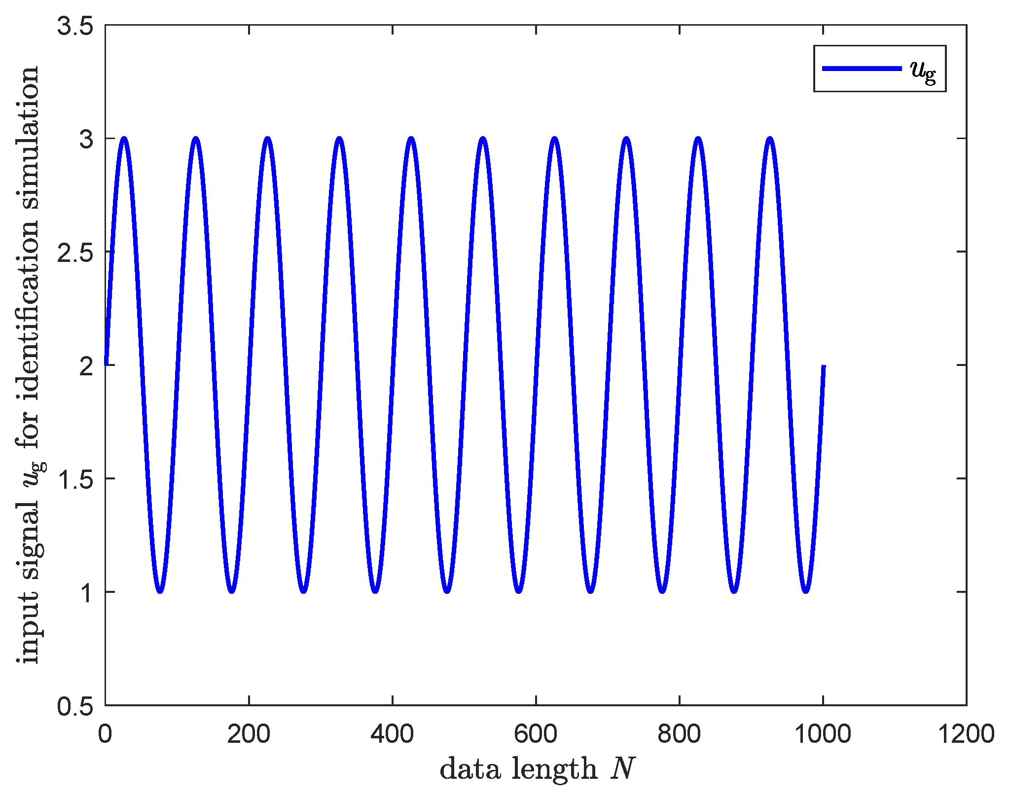
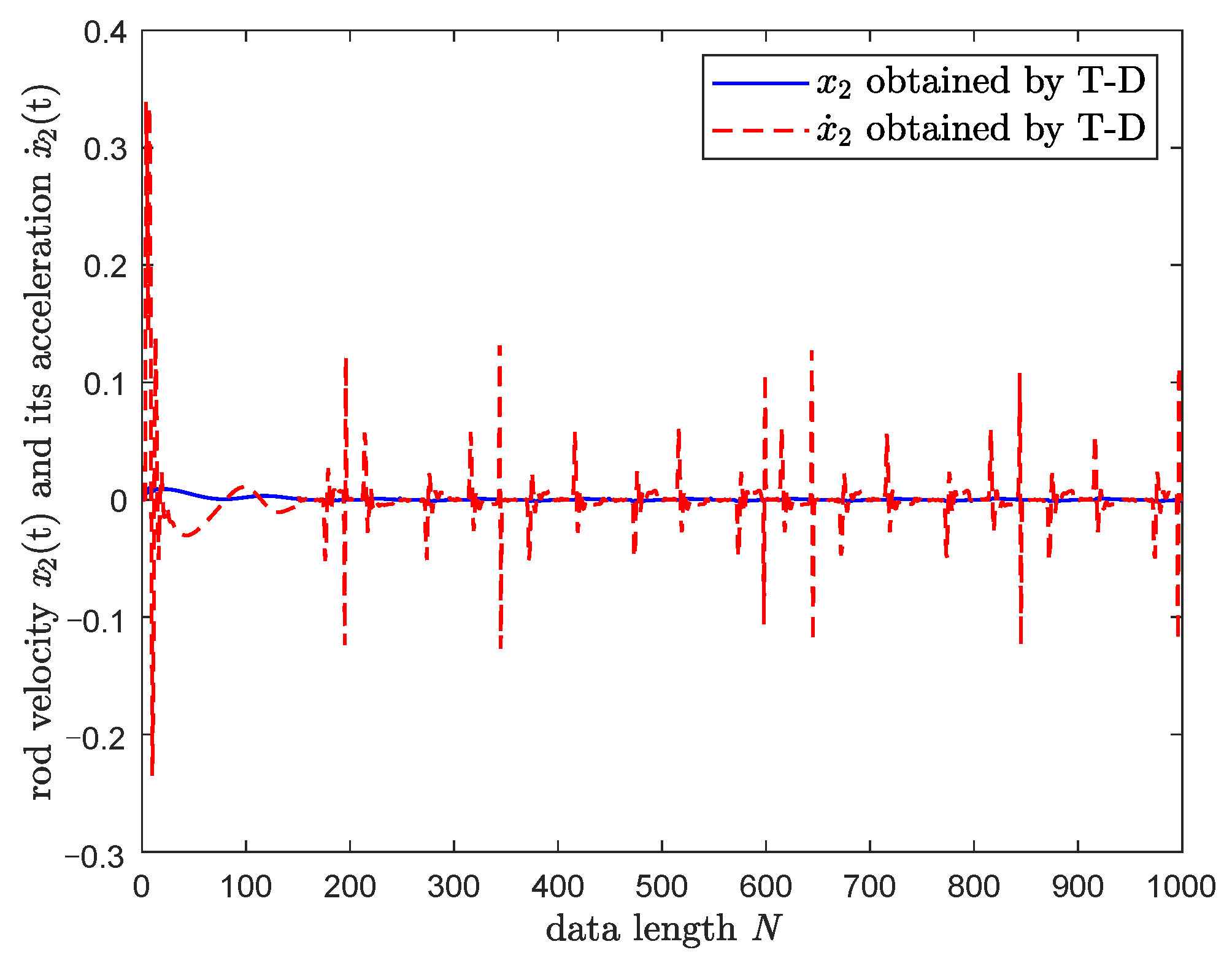
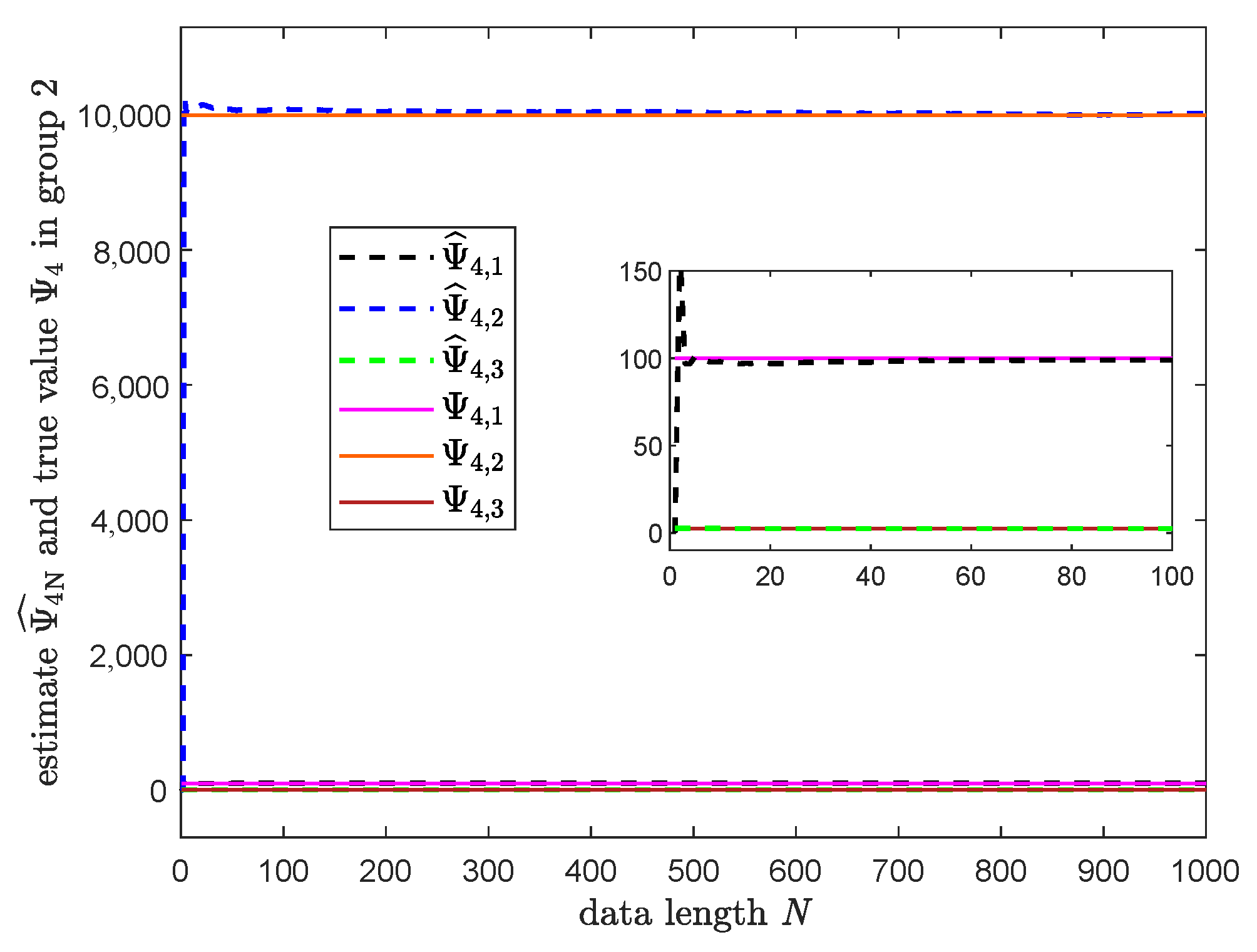
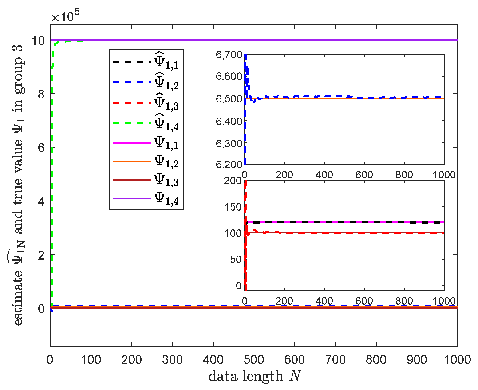
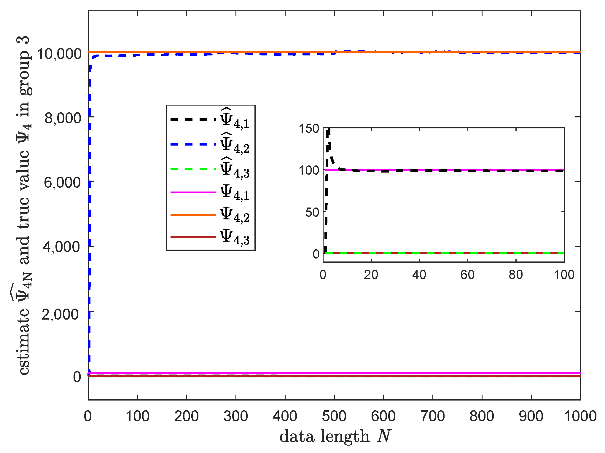
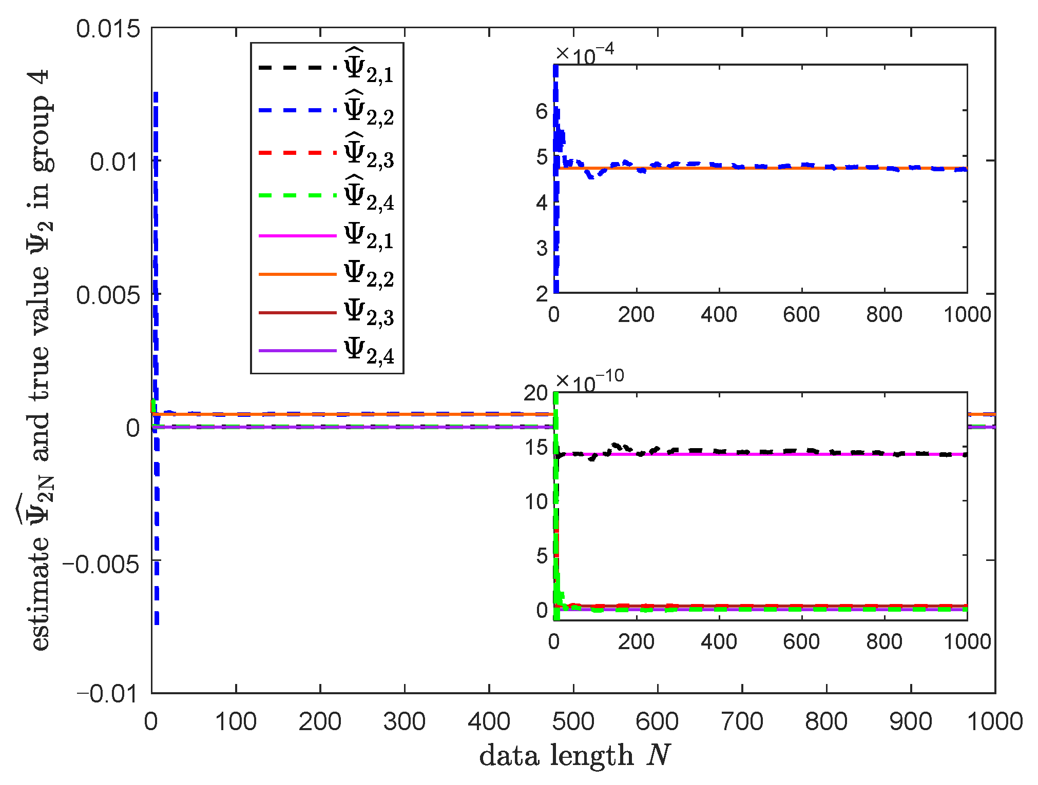
3.3. Numerical Simulation

MATLAB simulation software was used as the experimental tool. Referring to the nonlinear state space model established in Section 2.3:

$$\begin{array}{ccc}\dot{x}\left(t\right)\hfill & =& f(t,x(t),u(t\left)\right),\hfill \\ y\left(t\right)\hfill & =& h(t,x(t\left)\right).\hfill \end{array}$$

(55)

In the simulation, (55) was discretized by the fourth-order Runge–Kutta method(R-K), the sampling step h was taken as 0.01 s, and its implementation was as in (56).

$$\begin{array}{ccc}{x}_{k+1}\hfill & =& x_k+\frac{h}{6}({\alpha }_1+2{\alpha }_2+2{\alpha }_3+{\alpha }_4)\hfill \\ {\alpha }_1\hfill & =& f(t_k,x_k)\hfill \\ {\alpha }_2\hfill & =& f(t_k+\frac{h}{2},x_k+\frac{h}{2}{\alpha }_1)\hfill \\ {\alpha }_3\hfill & =& f(t_k+\frac{h}{2},x_k+\frac{h}{2}{\alpha }_2)\hfill \\ {\alpha }_4\hfill & =& f(t_k+h,x_k+h{\alpha }_3)\hfill \end{array}$$

(56)

The input of the system is $u_g=2+sin\left(2\pi t\right)$ in Figure 3, the simulation data of system parameters are shown in

Table 1. Summary table of system parameters.

Symbol	Physical Implication	Value
$K_{sv}$	Servo valve amplification factor	0.00025
${\omega }_{sv}$	Servo valve natural frequency	100
${\zeta }_{sv}$	Servo valve damping ratio	0.5
$K_p$	Proportional controller factor	1
$K_f$	Displacement sensor gain	40
$A_1$	Effective area of the piston on the left side	0.0085
$A_2$	Effective area of the piston on the right side	0.004
$C_{ip}$	Internal leakage factor	$3\times {10}^{-11}$
$C_{ep}$	External leakage factor	0
${\beta }_e$	Effective bulk modulus of elasticity	700,000,000
$K_t$	Spring stiffness	1,000,000
m	Total mass	120
B	Viscous damping factor	6000
$F_f$	Stribeck friction	0
$F_L$	External force	4000
$V_{01}$	Given by (12)	0.11
$V_{02}$	Given by (13)	0.09
$V_{L1}$	Given by (12)	0
$V_{L2}$	Given by (13)	0
$C_d$	Orifice flow factor	0.6
W	Orifice area gradient	0.03
$\rho$	Oil density	880
$p_s$	System oil supply pressure	12

, and total times $T=10$ s, $x_1\left(t\right)$, $x_3\left(t\right)$, $x_4\left(t\right)$ and $x_5\left(t\right)$ were obtained from (56). The data length was $N=T/h=1000$.

T-D parameters were $r=100$ and $h_0=0.05$. In order to obtain the first-order differentiation, $x_1\left(t\right),x_3\left(t\right),x_4\left(t\right)$ and $x_5\left(t\right)$ were used as the input signals of T-D to obtain the piston rod velocity data ${\dot{x}}_1\left(t\right)=x_2\left(t\right)$, the hydraulic cylinder left and right chamber pressure derivative data ${\dot{x}}_3\left(t\right)$ and ${\dot{x}}_4\left(t\right)$, and the servo valve velocity data ${\dot{x}}_5\left(t\right)=x_6\left(t\right)$. To obtain the second-order differentiation, $x_2\left(t\right)$ and $x_6\left(t\right)$ obtained by T-D serve as the input signal of T-D, and the corresponding differentiation signals ${\dot{x}}_2\left(t\right)$ and ${\dot{x}}_6\left(t\right)$ were obtained, respectively.

Afterwards, the parameter estimates were obtained on the basis of the identification algorithm in Section 3.2. In this experiment, the Coulomb friction factor $f_c$ was taken as 5 and the viscous friction factor $f_v$ was taken as 20; neglecting the Stribeck friction parameter $f_s$, (26) and (27) became:

$$\begin{array}{ccc}\hfill {{\rm Y}}_1& =& [{\dot{x}}_2,x_2,\mathrm{sign}\left(x_2\right),x_1],\hfill \end{array}$$

(57)

$$\begin{array}{ccc}\hfill {\Psi }_1& =& {[m,B+f_v,f_c,K_t]}^T.\hfill \end{array}$$

(58)

To demonstrate the effect of T-D, $y\left(t\right)$ in (55) is expanded, adding the results $x_2\left(t\right)$ and $x_6\left(t\right)$ from R-K. $x_2\left(t\right)$ and $x_6\left(t\right)$ obtained by R-K are only used for comparison and not for other uses in this paper. The experimental results are as follows:

The identification results are summarized in

Table 2. Summary of identification results.

Parameter	True Value	Estimated Value
${\Psi }_{1,1}$	120	120.04
${\Psi }_{1,2}$	6025	6027.50
${\Psi }_{1,3}$	5	4.95
${\Psi }_{1,4}$	$1\times {10}^6$	$0.99\times {10}^6$
${\Psi }_{2,1}$	$1.43\times {10}^{-9}$	$1.42\times {10}^{-9}$
${\Psi }_{2,2}$	$6.07\times {10}^{-4}$	$6.068\times {10}^{-4}$
${\Psi }_{2,3}$	$3\times {10}^{-11}$	$2.99\times {10}^{-11}$
${\Psi }_{2,4}$	0	$2.75\times {10}^{-13}$
${\Psi }_{3,1}$	100	99.85
${\Psi }_{3,2}$	10,000	10,014
${\Psi }_{3,3}$	2.50	2.5012

. Data differentiation processes by T-D are shown in Figure 4, Figure 5, Figure 6, Figure 7, Figure 8 and Figure 9. Parameter identification processes are shown in Figure 10, Figure 11 and Figure 12. From Figure 4 and Figure 8, it can be seen that T-D can obtain more satisfactory differential data. From Figure 10, Figure 11 and Figure 12, it is known that the system parameters can be identified based on T-D and the least squares recursive algorithm.

Remark 2.

The identification algorithm in this paper is based on a mathematical model of a hydraulic system. It can be applied to other hydraulic systems by making appropriate adjustments as long as the mathematical model is established.

4. Experimental Analysis of Health State Evaluation

To realize the health state evaluation of the hydraulic system, first, the monitoring data under the same operating condition were used as the basis to classify the health states through feature extraction and analysis; then, the identification algorithm in Section 3.2 was used to obtain the range of system parameters for different health states; finally, the data under the variable operating condition were captured for parameter identification to obtain system parameters, which were compared with the system parameter range, and then we evaluated which health state the system is in. Referring to [19,20], the hydraulic system health states can be classified as health, sub-health, average, deterioration and fault.

Among the system parameters in Table 1, $C_d$, W, $\rho$, $K_{sv}$, $C_{ip}$, $C_{ep}$, $f_c$ and $f_v$ vary with the health state and are variable; the rest of the parameters were invariant in the experiment.

4.1. Analysis of Data

By reviewing a large amount of literature, it is clear that piston rod displacement, as the actual output of the hydraulic system, can be used as a measure of the health status of the hydraulic system. First, capturing multiple groups of $x_1$, $x_3$, $x_4$ and $x_5$ under the same operating condition, $x_1$ was used for health state evaluation by signal processing. Then, $x_1$, $x_3$, $x_4$ and $x_5$ were labeled with different health states. The simulation step was $h=0.01$ s, the simulation time $T=10$ s, the data length $N=T/h=1000$, the input of the system was $u_g=2+sin\left(2\pi t\right)$, and 200 groups of $x_1$, $x_3$, $x_4$ and $x_5$ with different health states were obtained by changing the variable parameters. From expert experience, it is known that the mean value of $x_1$ gets smaller as the health status gets worse, so we can obtain four thresholds and label $x_1$, $x_3$, $x_4$ and $x_5$ with five health statuses. $x_1$ values in different health states are shown in Figure 13.

4.2. Evaluation of Health Status

The 200 groups of $x_1$, $x_3$, $x_4$ and $x_5$ labeled with five health states were obtained in the previous section, and the estimated values of system identifiable parameters were obtained by the identification algorithm in Section 3.2. Then, according to the labels, we can obtain the parameter range under different health states, the health state evaluation parameters consisting of variable parameters are $K_{sv},{\omega }_{sv}^2$, $\frac{C_{d}W}{\sqrt{\rho }}$, $f_c$, $B+f_v$, $C_{ip}$ and $C_{ep}$, and the parameter range is shown in the following table.

The range of parameters in

Table 3. The parameter range for health status evaluation.

Parameter	Health	Sub-Health	Average	Deterioration	Fault
$K_{sv}{\omega }_{sv}^2$	[2.6, 2.2]	[2.2, 1.7]	[1.7, 1.4]	[1.4, 1.0]	[1.0, 0.5]
$\frac{C_{d}W}{\sqrt{\rho }}$	↓ 1	↓	↓	↓	↓
$f_c$	[4, 10]	(10, 20]	(20, 45]	(45, 75]	(75, 120]
$B+f_v$	[6020, 6075]	(6075, 6150]	(6150, 6250]	(6250, 6400]	(6400, 6600]
$C_{ip}$	$3\times {10}^{-11}$	$3\times {10}^{-11}$	$3\times {10}^{-11}$	$3\times {10}^{-11}$	$3\times {10}^{-10}$
$C_{ep}$	0	0	0	0	$3\times {10}^{-10}$

¹ The ↓ symbol represents a downward trend for this parameter, but there is no clear range bound.

can be used as a basis for evaluating the health status.

In order to simulate the variable operating condition, we changed the input signal as follows.

$$u_g=0.5sin\left(5\pi t\right)+\left\{\begin{array}{cc}2,& \frac{T}{4}<t\le \frac{T}{2}\mathrm{or}t>\frac{3T}{4}\\ 2.5,& t\le \frac{T}{4}\mathrm{or}\frac{T}{2}<t\le \frac{3T}{4}\end{array}\right.$$

which is shown in Figure 14. $x_1$, $x_3$, $x_4$ and $x_5$ under $u_g$ were captured. Estimates of the variable parameters were obtained by R-K, T-D and the identification algorithms in Section 3.2. Then, by comparison with Table 3, we performed a health status evaluation. Five groups of simulation results are given as follows.

The five groups of parameter identification processes are shown in Figure 15, Figure 16, Figure 17, Figure 18, Figure 19, Figure 20, Figure 21, Figure 22, Figure 23, Figure 24, Figure 25, Figure 26, Figure 27, Figure 28 and Figure 29. The five groups of identification results and the results of the health status evaluation performed by comparing with Table 3 are shown in

Table 4. Results of Identification algorithm and health status evaluation.

Parameter Estimates	${\mathit{K}}_{\mathit{sv}}{\mathit{\omega }}_{\mathit{sv}}^2$	$\frac{{\mathit{C}}_{\mathit{d}}\mathit{W}}{\sqrt{\mathit{\rho }}}\times {10}^4$	${\mathit{f}}_{\mathit{c}}$	$\mathit{B}+{\mathit{f}}_{\mathit{v}}$	${\mathit{C}}_{\mathit{ip}}\times {10}^{11}$	${\mathit{C}}_{\mathit{ep}}\times {10}^{13}$	Evaluation Results
Group 1	1.96	$5.51$	14.64	6098.00	$2.94$	$8.68$	Sub-health
Group 2	2.49	$5.70$	4.67	6021.31	$3.01$	$2.45$	Health
Group 3	0.79	$3.74$	99.48	6496.67	$29.15$	3010	fault
Group 4	1.6	$4.74$	29.78	6183.32	$2.99$	$2.06$	Average
Group 5	1.19	$4.75$	60.44	6297.15	$3.03$	$3.20$	Deterioration

.

5. Conclusions

The health state of a hydraulic system depends largely on the system parameters, and the change of parameters will definitely affect the system’s performance. Based on the nonlinear mathematical model of a hydraulic system, first, the nonlinear model is transformed into least-squares identifiable format through parameter linearization. The fourth-order Runge–Kutta method is used to obtain the measurable data of the system, and the differential data of measurable data are obtained by a tracking-differentiator (T-D). The least-squares recursive algorithm is used to estimate the system parameters. Second, under the same operating condition, the health state change is simulated by changing the variable parameters, so as to classify the measurable data and obtain the health state range of the variable parameters by an identification algorithm. Finally, under the variable operating condition, the estimates of variable parameters are obtained by the identification algorithm and compared with the health state range to evaluate which health state the system is in.

The health state graded evaluation method proposed in this paper focuses on the electro-hydraulic position servo system, and combines the use of both signal processing-based and model-based methods. In future work, on the one hand, the application of this method to other systems can be explored. On the other hand, we can also consider introducing a knowledge-based method to combine three methods to establish a health state evaluation method with a more complete algorithm and application for a broader range of areas.

References

1. Yu, Y.; Do, T.; Yin, B.; Ann, K.K. Improvement of energy saving for hybrid hydraulic excavator with novel powertrain. Int. J. Precis. Eng.-Manuf.-Green Technol. 2023, 10, 521–534. [Google Scholar] [CrossRef]
2. Fu, X.; Wang, R.; Zhao, Y. Intelligent decision-making model on the of hydraulic supports group advancing behavior to follow shearer. China Coal Soc. 2020, 45, 2065–2077. [Google Scholar]
3. Shi, Q.; He, L. A Model Predictive Control Approach for Electro-Hydraulic Braking by Wire. IEEE Trans. Ind. Inform. 2023, 19, 1380–1388. [Google Scholar] [CrossRef]
4. Qian, C.; Zhu, J.; Shen, Y.; Jiang, Q.; Zhang, Q. Deep Transfer Learning in Mechanical Intelligent Fault Diagnosis: Application and Challenge. Neural Process. Lett. 2022, 54, 2509–2531. [Google Scholar] [CrossRef]
5. Tian, X.; Wang, S.; Zhang, C. Performance degradation of hydraulic cylinder reciprocating seals. In Proceedings of the 2018 13th IEEE Conference on Industrial Electronics and Applications, Wuhan, China, 31 May–2 June 2018; pp. 2117–2122. [Google Scholar]
6. Zhou, M. Research Progress of Aircraft Hydraulic System Health Management. Hydraul. Pneum. Seals 2021, 41, 6–8+15. [Google Scholar]
7. Gajjar, S.; Kulahci, M.; Palazoglu, A. Real-time Fault Detection and Diagnosis Using Sparse Principal Component Analysis. J. Process Control 2018, 67, 112–128. [Google Scholar] [CrossRef]
8. Secrest, C.W.; Lorenz, R.D. Adaptive Decoupling of Nonideal Machine and Sensor Properties for Extraction of Fine Details When Using the Motor Drive as a Diagnostic Sensor. IEEE Trans. Ind. Appl. 2017, 53, 2925–2935. [Google Scholar] [CrossRef]
9. Guo, J.; Diao, J.-D. Prediction-Based Event-Triggered Identification of Quantized Input FIR Systems with Quantized Output Observations. Sci. China Inf. Sci. 2020, 63, 112201:1–112201:12. [Google Scholar] [CrossRef]
10. He, Y.; Guo, J. FIR Systems Identification Under Quantized Output Observations and A Large Class of Persistently Exciting Quantized Input. J. Syst. Sci. Complex. 2017, 30, 1061–1071. [Google Scholar] [CrossRef]
11. Liu, D.; Dai, S. Application of PHM Technology in Hydraulic Servo System. Avion. Technol. 2016, 47, 49–56. [Google Scholar]
12. Song, D.; Lv, C.; Qi, L.; Wang, J.; Wu, Y. Performance Assessment of Hydraulic System Based on Health Baselines and Mahalanobis Distance in Variable Conditions. Syst. Simul. Technol. 2017, 13, 201–208. [Google Scholar]
13. Qian, C.; Li, W.; Yu, Z.; Yu, W.; Tang, H. Research on the health condition assessment method of marine hydraulic system based on residual vectors. China Shiprep. 2017, 30, 44–47. [Google Scholar]
14. Guo, J.; Wang, X.; Xue, W.; Zhao, Y. System Identification with Binary-Valued Observations Under Data Tampering Attacks. IEEE Trans. Autom. Control 2021, 66, 3825–3832. [Google Scholar] [CrossRef]
15. Tan, S.; Guo, J.; Zhao, Y.; Zhang, J.-F. Adaptive Control with Saturation-Constrainted Observations for Drag-Free Satellites—A Set-Valued Identification Approach. Sci. China Inf. Sci. 2021, 64, 202202:1–202202:12. [Google Scholar] [CrossRef]
16. Yang, W.; Lang, Z.; Tian, W. Condition monitoring and damage location of wind turbine blades by frequency response transmissibility analysis. IEEE Trans. Ind. Electron. 2015, 62, 6558–6564. [Google Scholar] [CrossRef]
17. Wang, X.; Jiang, B.; Lu, N.; Zhang, C. Dynamic fault prognosis for multivariate degradation process. Neurocomputing 2018, 275, 1112–1120. [Google Scholar] [CrossRef]
18. Li, P. Research on Performance Change Trend Prediction Method of Key Components of Aircraft Hydraulic System. Master’s Thesis, Shenyang Aerospace University, Shenyang, China, 2019. [Google Scholar]
19. Lin, Z. Study on Healthy State Assessment Technology for Aircraft Hydraulic System. Master’s Thesis, Shenyang Aerospace University, Shenyang, China, 2014. [Google Scholar]
20. Qi, J.; Wang, L.; Li, J.; Meng, Y. Method of comprehensive health assessment of the hydraulic system. Mach. Des. Manuf. 2016, 303, 64–68. [Google Scholar]
21. Jiang, W.; Zhou, J.; Zhu, Y.; Cui, X. Experimental research on sensitive characteristic parameter selection of hydraulic cylinder internal leakage fault. Hydraul. Pneum. 2014, 3, 119–124+129. [Google Scholar]
22. Zhang, L.; Lang, Z. Wavelet energy transmissibility function and its application to wind turbine bearing condition monitoring. IEEE Trans. Sustain. Energy 2018, 9, 1833–1843. [Google Scholar] [CrossRef]
23. Yao, Y. Research on Mechanical Fault Diagnosis Based on Self-Sensing Properties of Motor Drive System. Ph.D. Thesis, Huazhong University of Science and Technology, Wuhan, China, 2020. [Google Scholar]
24. Guo, L.; Li, N.; Jia, F.; Lei, Y.; Lin, J. A recurrent neural network based health indicator for remaining useful life prediction of bearings. Neurocomputing 2017, 240, 98–109. [Google Scholar] [CrossRef]
25. Liao, L.; Jin, W.; Pavel, R. Enhanced restricted Boltzmann machine with prognosability regularization for prognos-tics and health assessment. IEEE Trans. Ind. Electron. 2016, 63, 7076–7083. [Google Scholar] [CrossRef]
26. Zhu, Y.; Li, G.; Tang, S.; Wang, R.; Su, H.; Wang, C. Acoustic signal-based fault detection of hydraulic piston pump using a particle swarm optimization enhancement CNN. Appl. Acoust. 2022, 192, 108718. [Google Scholar] [CrossRef]
27. Liu, J.; Yang, H.; He, J.; Sheng, Z.; Chen, S. Unbalanced Fault Diagnosis Based on an Invariant Temporal-Spatial Attention Fusion Network. Comput. Intell. Neurosci. 2022, 2022, 1875011. [Google Scholar] [CrossRef] [PubMed]
28. Hou, D.; Cao, M. A hybrid deep learning model approach for performance index prediction of mechanical equipment. Meas. Sci. Technol. 2022, 33, 105108. [Google Scholar] [CrossRef]
29. Zhao, Z.; Jiang, W.; Gao, W. Health Evaluation and Fault Diagnosis of Medical Imaging Equipment Based on Neural Network Algorithm. Comput. Intell. Neurosci. 2021, 2021, 6092461. [Google Scholar] [CrossRef]
30. Gao, B.; Guan, H.; Zhang, W.; Shen, W.; Ye, Y. Three kinds of improved designs and comparative analysis based on active disturbance rejection controller. J. Mech. Sci. Technol. 2023, 37, 965–976. [Google Scholar] [CrossRef]
31. Feng, H.; Ma, W.; Yin, C.; Cao, D. Trajectory control of electro-hydraulic position servo system using improved PSO-PID controller. Autom. Constr. 2021, 127, 103722. [Google Scholar] [CrossRef]
32. Zhou, R.; Meng, L.; Yuan, X.; Qiao, Z. Research and experimental analysis of hydraulic cylinder position control mechanism based on pressure detection. Machines 2022, 10, 1. [Google Scholar] [CrossRef]
33. Alleyne, A.; Liu, R. A simplified approach to force control for electro-hydraulic systems. Control Eng. Pract. 2000, 8, 1347–1356. [Google Scholar] [CrossRef]
34. Wang, C.; Ding, F.; Li, Q.; Yang, Q. Research on dynamic characteristics of asymmetric cylinder controlled by symmetric four-way valve. China Mech. Eng. 2004, 15, 3–6. [Google Scholar]
35. Liang, Q.; Gao, J.; Liu, F.; Wang, K.; Zhang, H.; Wang, Z.; Su, D. Application of Hardware-in-the-Loop Simulation Technology in the Development of Electro-Hydraulic Servo System Control Algorithms. Electronics 2022, 11, 3850. [Google Scholar] [CrossRef]
36. Luo, Z. Particle Filtering Based on Fault Diagnosis of Electro Hydraulic Position Servo System. Master’s Thesis, Yanshan University, Qinhuangdao, China, 2014. [Google Scholar]
37. Shi, Z.; Gu, F.; Lennox, B.; Ball, A.D. The development of an adaptive threshold for model-based fault detection of a nonlinear electro-hydraulic system. Control Eng. Pract. 2005, 13, 1357–1367. [Google Scholar] [CrossRef]
38. Armstrong-Hélouvry, B.; Dupont, P.; De Wit, C.C. A survey of models, analysis tools and compensation methods for the control of machines with friction. Automatica 1994, 30, 1083–1138. [Google Scholar] [CrossRef]
39. Grotjahn, M.; Daemi, M.; Heimann, B. Friction and rigid body identification of robot dynamics. Int. J. Solids Struct. 2001, 38, 1889–1902. [Google Scholar] [CrossRef]
Figure 1. Configuration of electro-hydraulic position servo system.
Applsci 13 06052 g001
Figure 2. System of four-way slide valve-controlled asymmetric cylinder.
Applsci 13 06052 g002
Figure 3. The input signal for the identification algorithm analysis.
Applsci 13 06052 g003
Figure 4. x 1 and its differential signal x 2 .
Applsci 13 06052 g004
Figure 5. x 2 and its differential signal x ˙ 2 .
Applsci 13 06052 g005
Figure 6. x 3 and its differential signal x ˙ 3 .
Applsci 13 06052 g006
Figure 7. x 4 and its differential signal x ˙ 4 .
Applsci 13 06052 g007
Figure 8. x 5 and its differential signal x ˙ 6 .
Applsci 13 06052 g008
Figure 9. x 6 and its differential signal x ˙ 6 .
Applsci 13 06052 g009
Figure 10. Results of the identification algorithm for Ψ 1 .
Applsci 13 06052 g010
Figure 11. Results of the identification algorithm for Ψ 2 .
Applsci 13 06052 g011
Figure 12. Results of the identification algorithm for Ψ 4 .
Applsci 13 06052 g012
Figure 13. x 1 in different health states.
Applsci 13 06052 g013
Figure 14. The input signal for health status evaluation.
Applsci 13 06052 g014
Figure 15. Identification results of the first group for Ψ 1 .
Applsci 13 06052 g015
Figure 16. Identification results of the first group for Ψ 2 .
Applsci 13 06052 g016
Figure 17. Identification results of the first group for Ψ 4 .
Applsci 13 06052 g017
Figure 18. Identification results of the second group for Ψ 1 .
Applsci 13 06052 g018
Figure 19. Identification results of the second group for Ψ 2 .
Applsci 13 06052 g019
Figure 20. Identification results of the second group for Ψ 4 .
Applsci 13 06052 g020
Figure 21. Identification results of the third group for Ψ 1 .
Applsci 13 06052 g021
Figure 22. Identification results of the third group for Ψ 2 .
Applsci 13 06052 g022
Figure 23. Identification results of the third group for Ψ 4 .
Applsci 13 06052 g023
Figure 24. Identification results of the fourth group for Ψ 1 .
Applsci 13 06052 g024
Figure 25. Identification results of the fourth group for Ψ 2 .
Applsci 13 06052 g025
Figure 26. Identification results of the fourth group for Ψ 4 .
Applsci 13 06052 g026
Figure 27. Identification results of the fifth group for Ψ 1 .
Applsci 13 06052 g027
Figure 28. Identification results of the fifth group for Ψ 2 .
Applsci 13 06052 g028
Figure 29. Identification results of the fifth group for Ψ 4 .
Applsci 13 06052 g029