Article

Research on the Structure Optimization Design of Automobile Intake Pipe

1
Mechanical and Electrical Engineering College, Hainan University, Haikou 570228, China
2
Light Industry Science and Engineering College, South China University of Technology, Guangzhou 510641, China
*
Author to whom correspondence should be addressed.
Appl. Sci. 2023, 13(11), 6505; https://doi.org/10.3390/app13116505
Submission received: 28 March 2023 / Revised: 8 May 2023 / Accepted: 24 May 2023 / Published: 26 May 2023
(This article belongs to the Topic Computational Fluid Dynamics (CFD) and Its Applications)

Abstract

:
As the front end of the intake system, the intake dirty pipe is responsible for delivering sufficient and stable air to the air filter. Therefore, in order to meet the requirements of low intake resistance, it is necessary to correspondingly improve the flow resistance performance of the intake dirty pipe. In this study, the main research object was the intake pipe in the intake system of gasoline engine vehicles, and the internal gas flow field was simulated and analyzed. The results show that there are clear discrete velocity regions at the inlet and elbow, which affect the uniformity of the overall fluid flow and cause a certain pressure loss. After structural optimization, the total pressure difference at the inlet and outlet of the pipeline was reduced by 22.67% compared to the original model, and the total pressure loss was significantly reduced. A simplified model was used to make samples of the intake dirty pipes before and after performance improvement, and flow resistance tests were conducted respectively. The difference between test data and simulation data is within a reasonable range, and the simulation results are relatively reliable.

1. Introduction

The increasing number of automobiles has led to a growing concern about energy consumption and environmental pollution. Therefore, it is particularly important to improve the energy efficiency of and reduce emissions in automobiles [1,2,3]. Improving the charging efficiency of the engine is essential for achieving full and effective combustion, which in turn reduces the emission of pollutants. Effective measures to improve charging efficiency include reducing air resistance during the intake and exhaust processes and selecting suitable valve timing. Researchers have conducted research on the intake system since the advent of automobiles. Giannakopoulos et al., studied the incompressible flow at a low Reynolds number in a laboratory engine intake duct based on Bovendeerd’s description of the flow development process in circular cross-section curved ducts, using direct numerical simulation [4,5]. Sekavčnik et al., proposed a method for determining key parameters to evaluate system operation in unsteady flow research, providing some reference for this study [6]. Most researchers focus on studying the intake and exhaust manifold. The intake and exhaust manifolds are usually bend pipes, and researchers have studied the effects of changing the structure and layout of the manifold on gas flow uniformity and cylinder volume efficiency to explore whether engine performance is improved [7,8,9,10,11,12,13,14,15]. Silva et al., showed in their latest research that the engine has higher volume efficiency at high speeds when the length of the intake manifold flow path is shorter [16]. Some researchers have conducted research on the acoustic characteristics of the intake manifold [17,18,19,20], which is essentially a change in the structure of the intake pipe to reduce intake noise by increasing sound-absorbing elements. They verified their findings through bench tests, providing some reference for the research method used in this study. Some researchers have studied the housing and filter element of air filters [21,22,23,24,25,26], attempting to improve their performance by changing the structure of a particular location or adjusting the relative position with other parts; however, only simulation analysis has been performed, without the experimental verification of the simulation results. Few researchers have analyzed and researched the intake pipe before and after the implementation of the air filter [27,28,29]. In their latest research, Xie analyzed the intake performance of a certain type of intake pipe, optimizing the air intake by adjusting the bending curvature and setting a guide groove at the inlet [30]. Subsequently, the optimized model was verified through simulation but not through physical experiments. This study mainly focuses on reducing the flow resistance of the engine intake system by optimizing the relevant structure of the intake pipe to improve intake efficiency. Moreover, the optimized model was subjected to flow resistance tests to verify the reliability of the simulation results.

2. Materials and Methods

Computational fluid dynamics (CFD) is an interdisciplinary subject involving fluid mechanics, mathematics, computer science, and engineering. It uses electronic computers and numerical methods to model streamline mechanical processes to obtain physical parameters such as pressure, velocity, and temperature, and their distribution in the flow field, so as to better understand the essence of fluid dynamics. The emergence of CFD provides new opportunities for the research of fluid mechanics, and also provides important support for the development of human society. With the rapid development of various general CFD software, users can use the software to analyze and predict the research object, and adjust the corresponding parameters through the calculation results to achieve the goal of optimal design.
Fluid dynamics is an important discipline to study physical phenomena. It is based on the laws of conservation of mass, momentum, and energy to explore the laws of movement and changes in substances under stress. It uses mathematical equations to describe the motion laws of things, and can be used to predict the motion state of things, so as to better understand the motion characteristics of things.
During the flow process, the fluid may have two distinct states: laminar flow and turbulence. The physicist Reynolds used the Reynolds number to describe the dimensionless parameters of these two types of flows:
R e = ρ v d μ
In Formula (1), Re represents the Reynolds number, ρ Is the density of the fluid, v is the velocity of the fluid, d is the characteristic scale, and μ is the viscosity of the fluid. In general, in engineering, the flow in a pipe is considered to be fully turbulent when the Reynolds number exceeds 4000. Turbulence intensity is defined as the root mean square of velocity fluctuations divided by the mean velocity, and for fully developed internal flow, the turbulence intensity I can be expressed using Formula (2):
I = 0.16 ( R e ) 1 8
The standard k-ε model is a widely used turbulence model that combines turbulence energy k and turbulence dissipation rate ε. The transport equations are combined and expressed in the form of functions to build a complete model. The standard k-ε model has good versatility, and its calculation amount is small; thus, it can be used in most scenarios. However, for some specific cases, such as curved streamline flow, strong swirl effect, etc., the calculation results deviate strongly from the actual situation. Based on the RNG k-ε model, we can process more accurate calculations of the turbulent dissipation rate and turbulent viscosity, so as to better solve the flow with a large bending streamline, and make the solution results of the equations closer to the actual situation. The realizable k-ε model is also based on the standard k-ε model. It is a modified model that can effectively simulate different types of flow such as shear flow, pipe flow, jet flow, separated flow, etc.
Considering the interrelation between the three modes, the standard k-ε model is the basis, and the other two are based on the standard k-ε model and are more refined. Considering the flow of the model and the conditions of computing resources, as well as the experience of relevant industry simulation workers, we adopted the realizable k-ε model to complete the numerical simulation calculation.

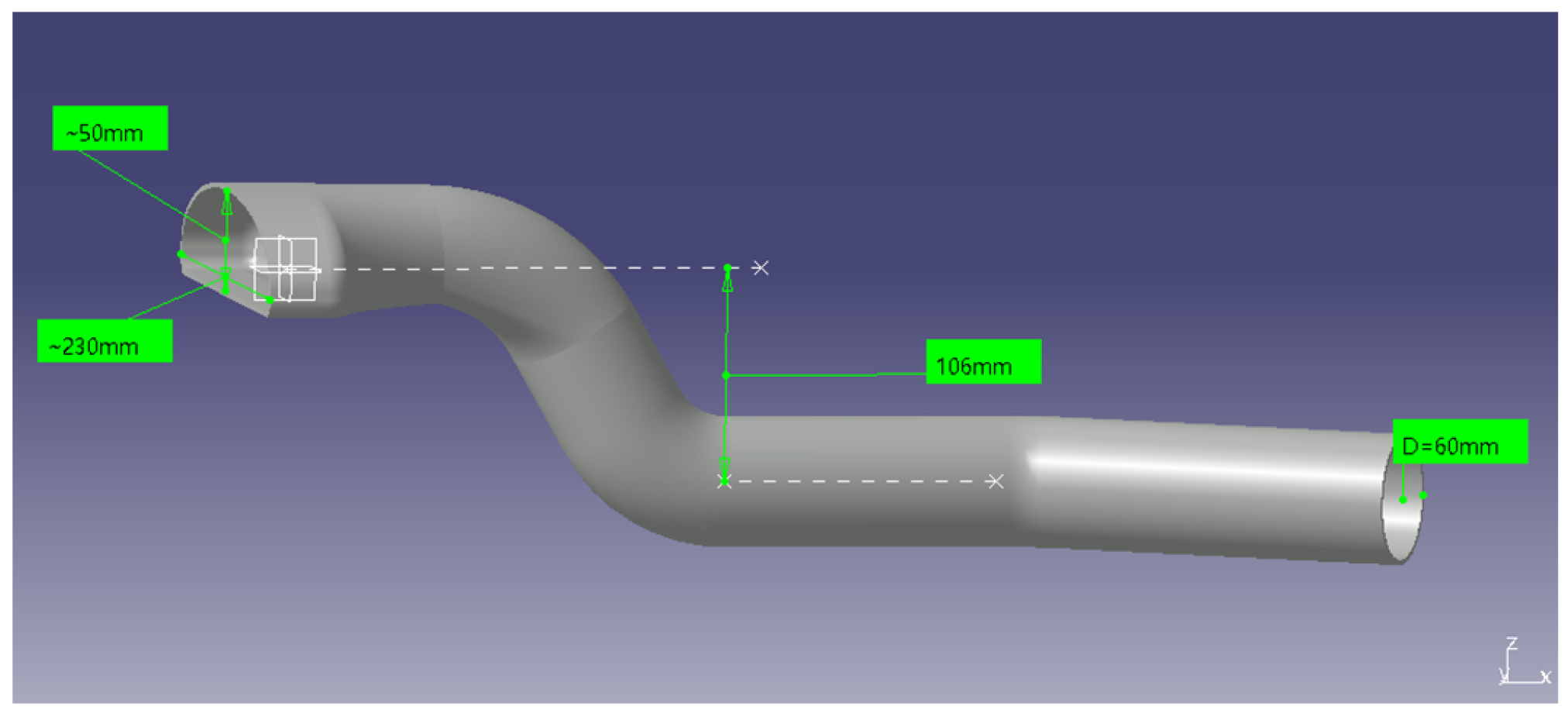
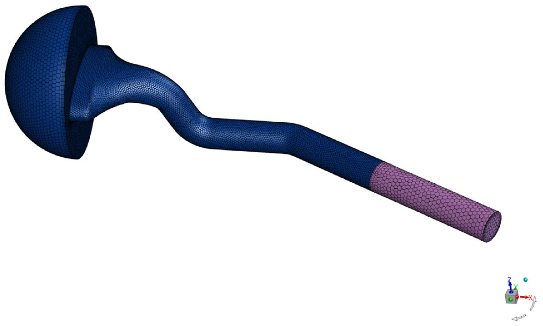
3. Model Establishment and Grid Division

This study used the intake dirty pipe of an air filter matched with a four-cylinder turbocharged engine of an undisclosed brand as the research object, and simulated and calculated the internal fluid flow. As the front end of the air intake system, the intake dirty pipe is connected to the air cleaner housing assembly. Its function is to stably deliver the inhaled ambient air to the air filter, effectively remove the moisture and impurities in the ambient air, and thus prevent operation wear. Figure 1 shows the three-dimensional model of the air filter assembly and intake pipe of an undisclosed brand.
In this study, CATIA was used for the geometric model design. In order to facilitate the following simulation and calculation work, it was necessary to properly simplify the intake pipe before modeling: we removed the resonant cavity connected above the intake pipe, and simplified the support on both sides of the intake pipe and the connection with the air filter. The simplified model only made appropriate changes to the external structure of the housing, without much simplification of the air intake port at the front of the intake pipe and the bends in the pipeline. Nevertheless, the simulation results still have reference values. The simplified three-dimensional geometric model of the intake pipe is shown in Figure 2. The maximum height difference in the front of the inlet dirty pipe is 50 mm, and the maximum width is 230 mm. The rear part is a circular pipe with an inner diameter of 60 mm, and the wall thickness of the entire intake dirty pipe is 2.5 mm.
Before meshing, it was necessary to extract the fluid domain from the inside of the intake dirty pipe. The internal surface of the intake dirty pipe was extracted through the generative shape design module, and the closed surface operation was performed on each surface after joining to obtain the fluid domain inside the pipe. Since the dirty air intake pipe is at the front of the air intake system, when air enters the pipe from the external environment, it does not enter the pipe directly perpendicular to the cross section of the pipe, but from the entire external area. Therefore, after extracting the fluid field inside the pipe, a hemispherical or square structure was added at the front of the air inlet, and a length of 3–4 times that of the inner diameter was appropriately added at the outlet of the inlet dirty pipe.
Next, we imported the fluid domain model into the fluent mesh module in ANSYS 2020 and completed the mesh settings. For this model, because some of its structural features are relatively complex, polyhedra-type mesh was used. Next, the geometric model was described accordingly; the geometric model was defined as a fluid region without gaps, and the interface types of all parts were defined as internal surfaces. Then, we added a boundary layer, the mesh type and size, and finally generated the volume mesh. In order to determine the grid independence, the generated volume grid was subjected to dense grid processing, and the final analysis results are not significantly different from those of the original grid. Figure 3 shows the generated grid model of the fluid domain of the air filter intake pipe, which is divided into 417,510 nodes and 101,407 cells.
Assuming the ambient temperature is 25 °C, the air density at this time was calculated from the air density table: ρ 1.1691 kg/m3, viscosity μ 1.834 × 10⁻⁵ kg/m−s. To obtain the air flow rate, it is necessary to know the intake air flow of the engine first. The formula for the maximum intake air flow of the engine is:
Q max = V d S max V e K
where Vd is the total displacement of the engine. This engine’s Vd =1.4 L; Smax is the speed corresponding to the maximum output power of the engine, which is Smax = 6000 rad/min; and Ve is the inflation efficiency of the engine. For supercharged engines, Ve is 1.3–1.5, and in this paper, Ve = 1.5; K is constant, and for four-stroke engines, K = 2000. It can be calculated that the maximum intake flow of the engine is 6.3 m3/min.
For the characteristic scale, when the fluid flows through the circular pipe, its value is the inner diameter of the circular pipe. For the non-circular section, its hydraulic diameter is usually calculated and defined as the characteristic scale. The formula is:
d = 4 S C
where S is the section area and C is the perimeter of the section. It can be calculated that d = 76 mm. According to Formula (1), the Reynolds number can be calculated as 53,244, which means high Reynolds number turbulence. We set the turbulence model as the realizable k-ε model, set the wall function as the standard wall function, and then set the physical parameters of the fluid. The boundary conditions are defined as pressure inlet and mass flow outlet, where the pressure inlet needs to be set with turbulence intensity. The inlet and outlet areas are set as shown in Figure 4. According to Formula (2), the turbulence intensity can be calculated as 4.11%. The detailed boundary condition parameter settings are shown in Table 1.
It should be noted that the FLUENT is based on the finite volume method principle, which divides the continuous region into a series of non-repeating control volumes and calculates and integrates them separately to obtain a similar solution. This study used the common SIMPLE solution algorithm, which assumes a velocity distribution and calculates an initial pressure value based on that distribution, which is applied to the momentum equation to obtain the velocity values. Then, the velocity values are substituted into the continuity differential equation to solve the pressure correction differential equation and finally obtain the converged results.
Subsequently, the residual convergence range was set to 10-6, and parameter monitoring was carried out at the inlet and outlet sections of the pipeline. Here, the speed was selected as a reference. After the setting was completed, mixed initialization was carried out, and the iteration number was set to 1000 times. Then, the calculation began, monitoring the residual convergence process and the velocity fluctuations of the inlet and outlet sections. Finally, when the calculation reached 665 times, the residual converges and the calculation ended.

4. Results

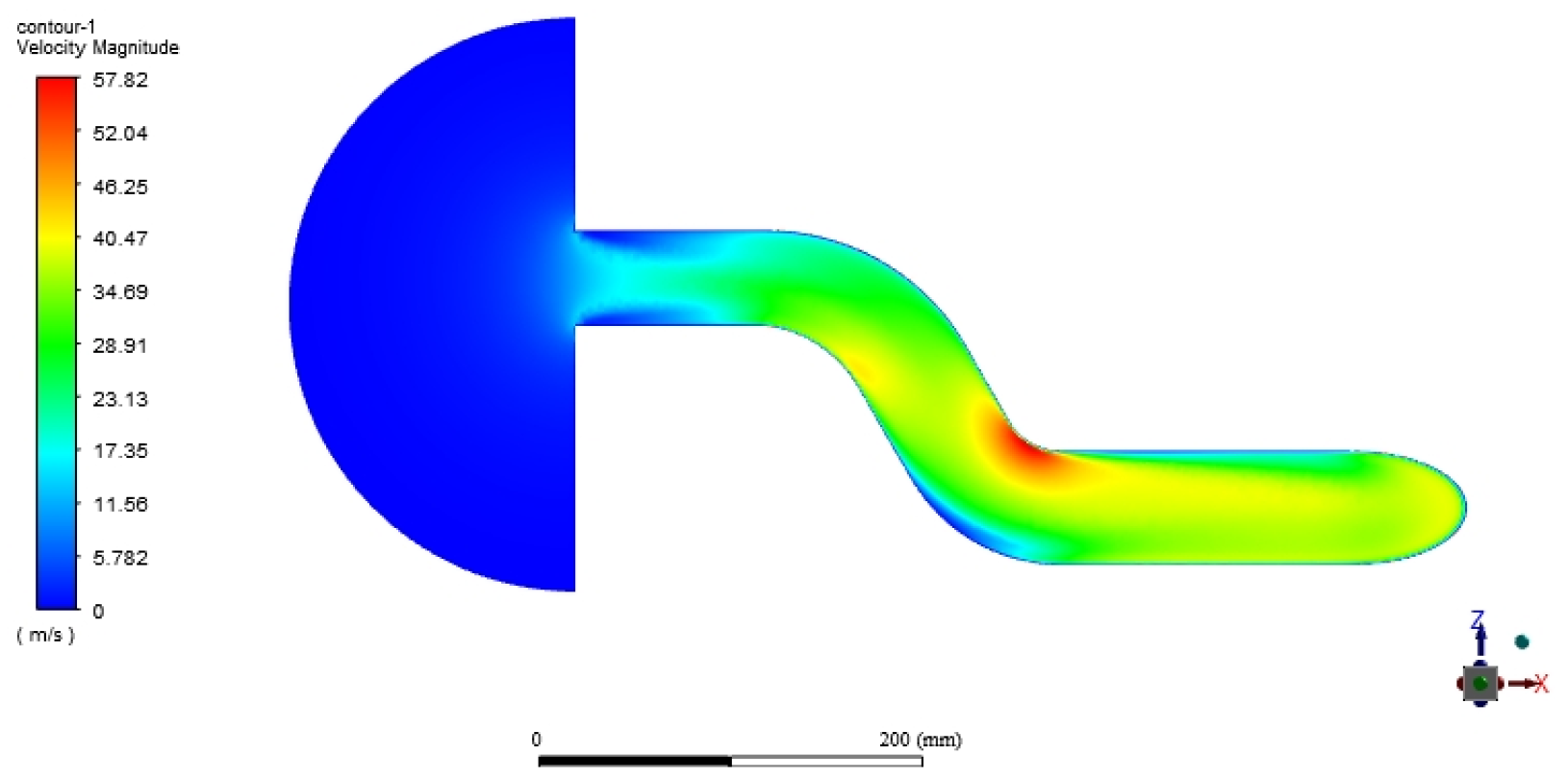
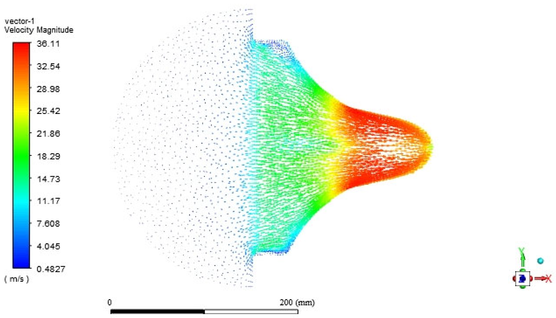
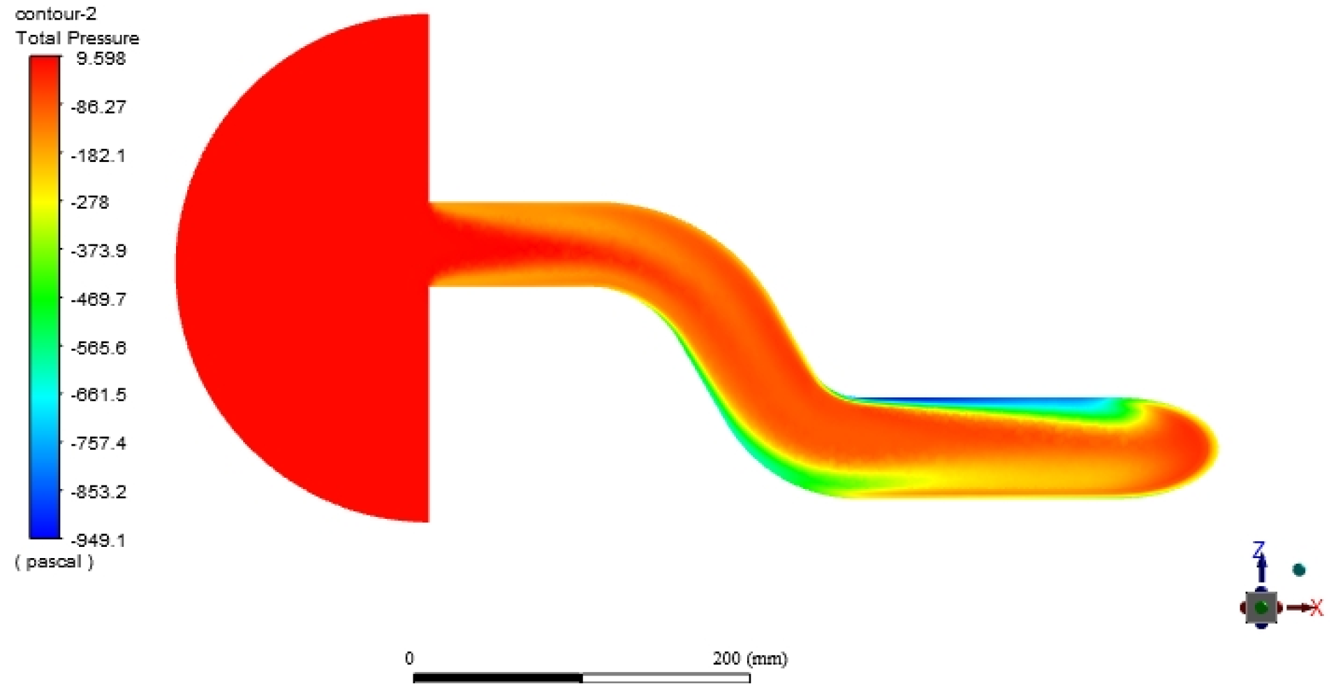
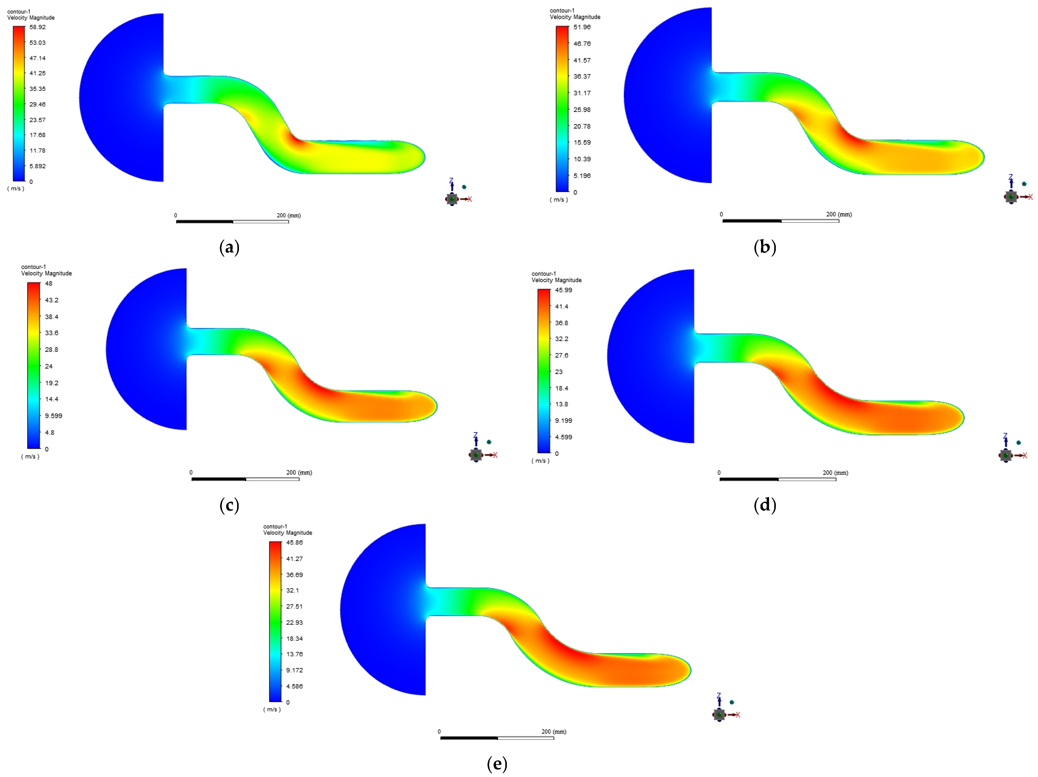
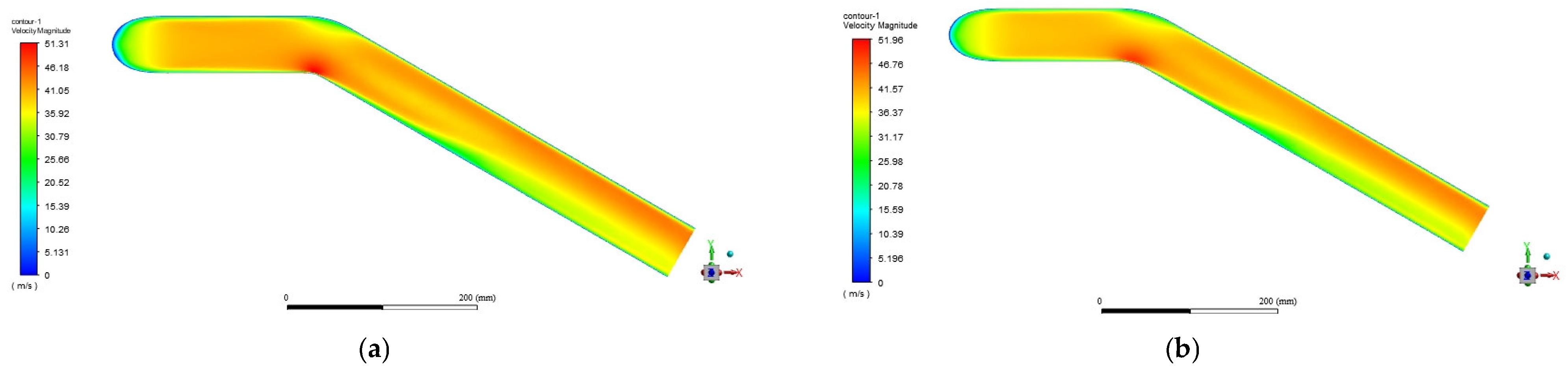
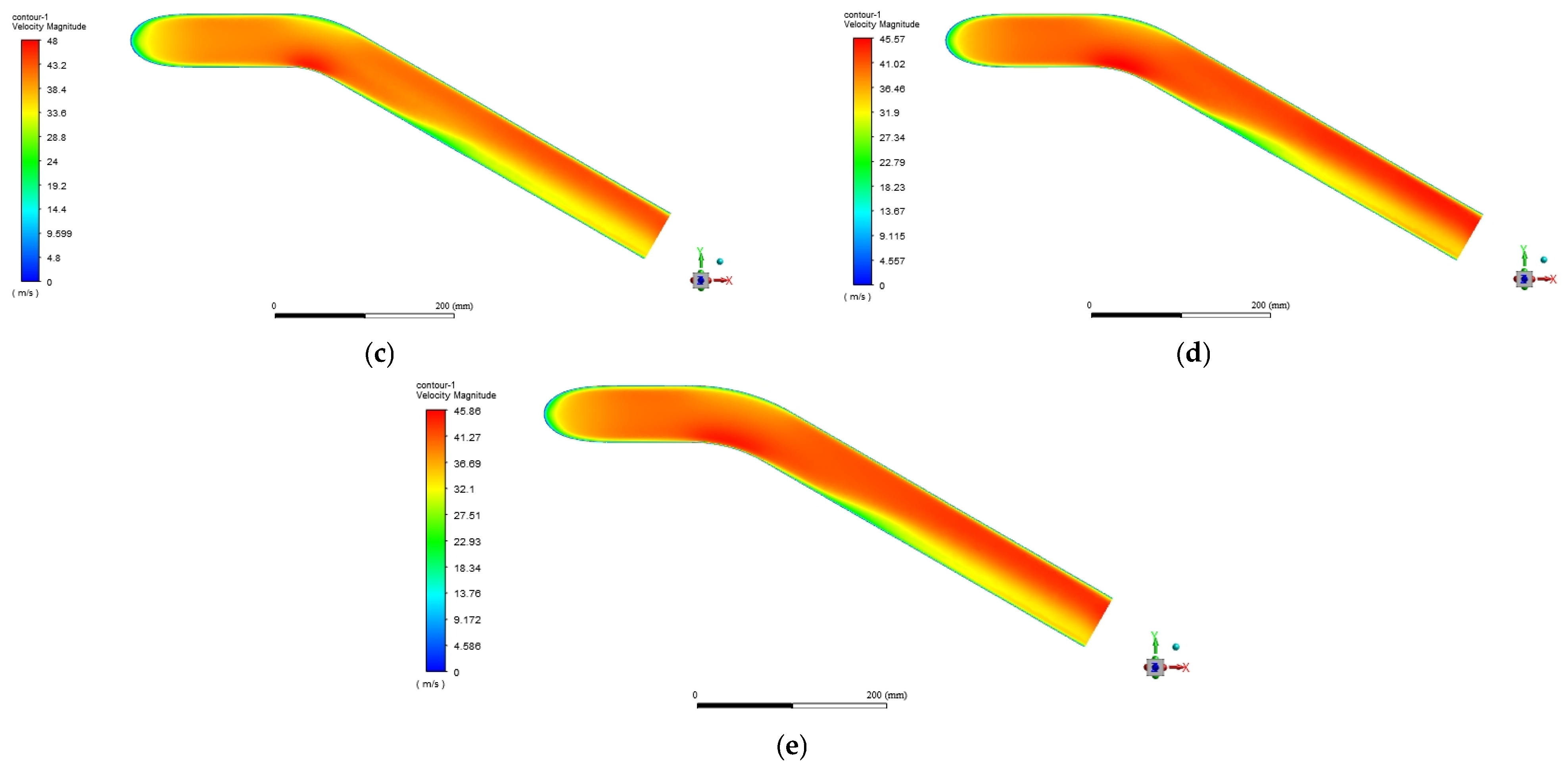
4.1. Numerical Simulation Results and Analysis of the Model

In the flow field, characteristics such as resistance are closely related to the velocity and pressure of the flow field. Therefore, when analyzing the flow field in post-processing, we conducted in-depth research on the two aspects of velocity and pressure to obtain more accurate results, and combined the actual situation, analyzed the characteristics such as resistance, and improved the flow field characteristics through performance improvement design. In order to describe the motion characteristics of the flow field more accurately, we selected a plane section that can reflect the flow characteristics as a reference to analyze the flow field more in depth.
Figure 5 shows the partial velocity contour of the air inlet at the front of the dirty air inlet pipe with y = 0 mm and an xoz section. It can be seen from the figure that when air enters the air inlet from the external environment, there is a velocity gradient change, and the air flow near the pipe wall is low, which will lead to an unsmooth air inlet. A clear sudden change in speed occurs at the second pipe bend, which leads to an excessive pressure loss at the bend. Figure 6 shows the velocity contour at the rear end of the inlet dirty pipe with z = −106 mm and an xoy section. It can be seen from the figure that the speed mutation region also occurs at the bending part, which affects the overall fluid flow uniformity and causes pressure loss. According to the two figures, the maximum velocity appears at the bend of the pipe, with the values of 57.8 m/s and 52.6 m/s. This is due to the sudden change in the flow channel inside the flow field and the effect of the pressure difference, which leads to the acceleration of the air flow, resulting in this maximum value. Figure 7 shows the velocity vector diagram of the inlet part at the front of the inlet dirty pipe with z = 0 mm and an xoy section. It can be seen from the figure that the velocity uniformity of the flow field at the front of the inlet dirty pipe is poor, and the local structure produces a backflow area, resulting in a pressure loss.
Figure 8 shows the pressure contour of the inlet part at the front of the inlet dirty pipe with y = 0 mm and an xoz section. It can be seen from the figure that there are pressure gradient changes at the inlet and at the bend, and the pressure gradient changes at the second bend are more obvious, which is due to the sharp increase in the speed at the bend, which is consistent with the analysis in Figure 5. Figure 9 shows the pressure contour at the rear end of the inlet dirty pipe with z = −06 mm and an xoy section. It can be seen from the figure that the pressure gradient change area also occurs at the rear end of the pipe, which is also caused by the speed surge at the bend, which is consistent with the analysis in Figure 6.
According to the two figures, the inlet and outlet pressures are significantly different due to the uneven distribution of inlet air and the bending of the pipe. According to the calculation results, the average total pressure difference between the inlet and outlet of the original model is 230.01 Pa.

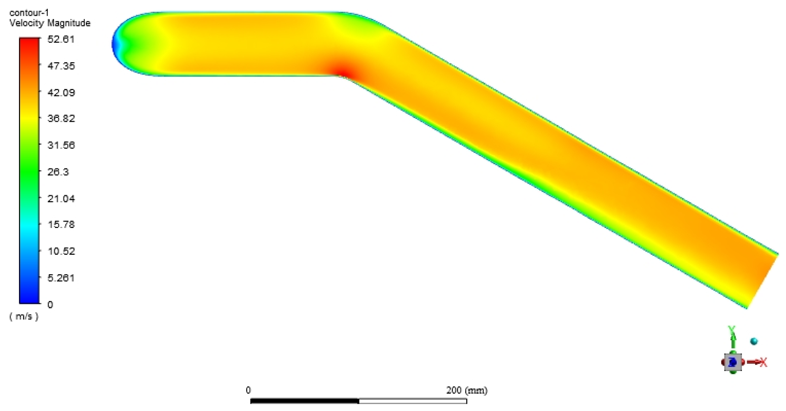
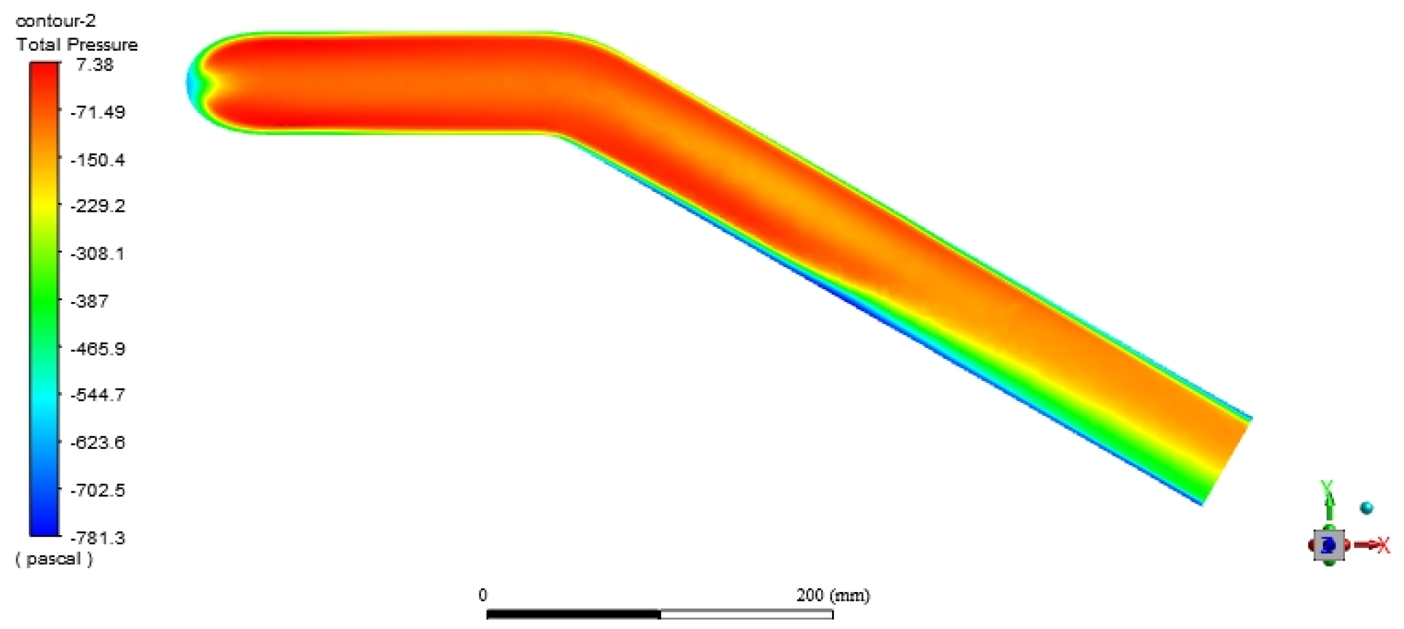
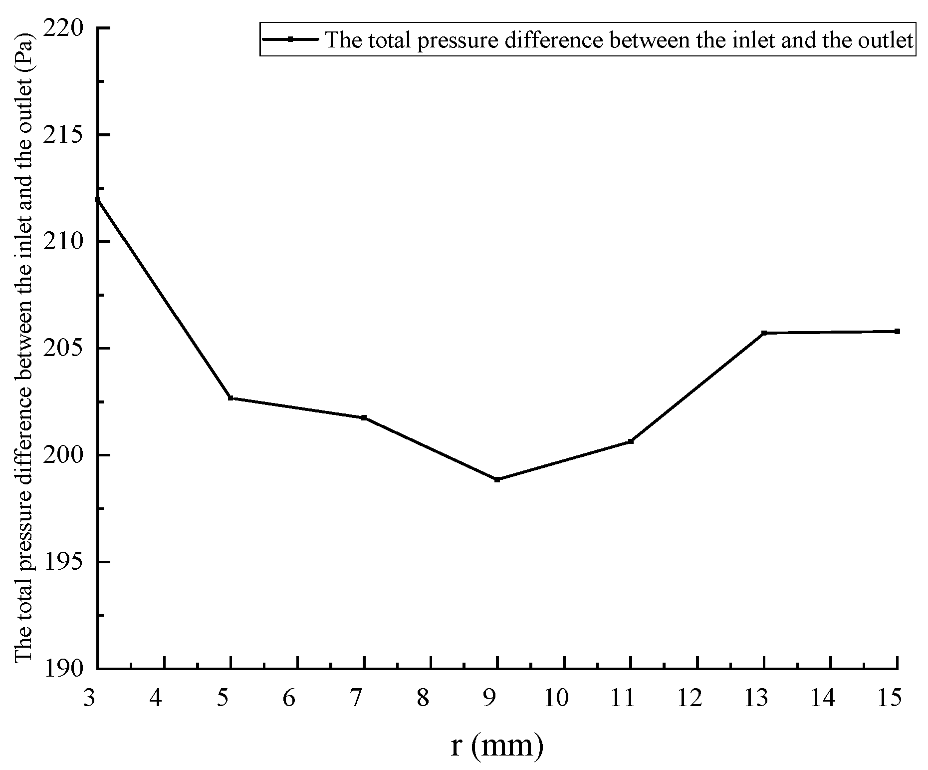
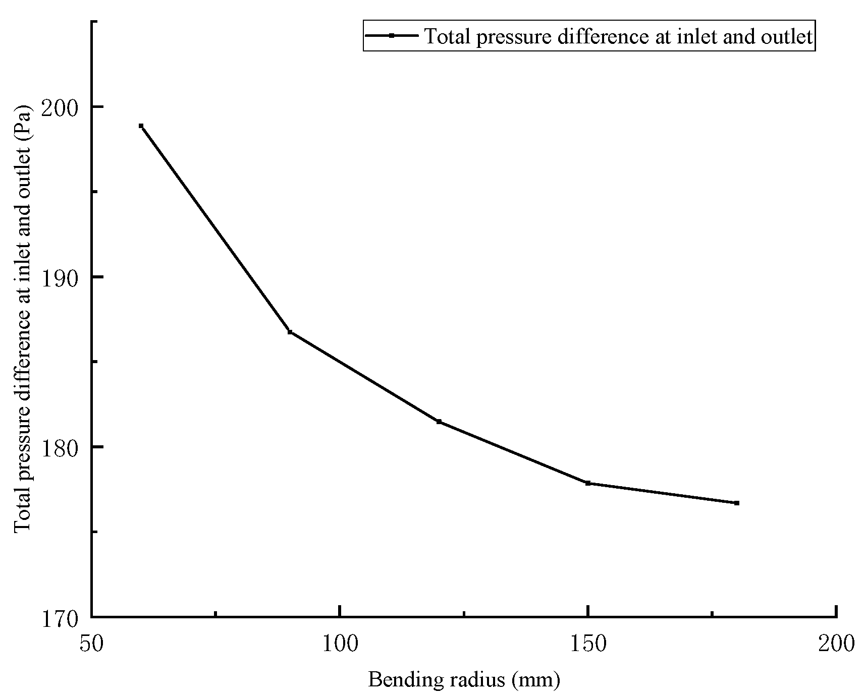
4.2. Optimization and Analysis of Intake Dirty Pipe Structure

When air enters the pipe, the pressure near the wall of the pipe is large due to the air entering from all directions, resulting in a velocity gradient, which affects the flow uniformity, resulting in an excessive pressure difference at the inlet and outlet. In order to increase the flow uniformity of the air and reduce the total pressure difference at the inlet and outlet, the front of the pipe was locally optimized by adding a trumpet structure. The optimized two-dimensional plane diagram is shown in Figure 10.
By changing the radius of the trumpet structure at the inlet, the flow state at the inlet is explored and the pressure change at the inlet and outlet is monitored. Due to the inner diameter of the intake pipe being 60 mm and the wall thickness being 2.5 mm, in order to avoid the influence of the horn-shaped structure on air flow into the intake pipe and the inability to match other components due to the large lateral width of the intake pipe, we increased the horn-shaped radius from 3 mm to 15 mm, with an interval of 2 mm in order to analyze the changes in radius on inlet flow uniformity and inlet/outlet pressure difference, and obtain the optimal radius. Compared to Mariotti’s spline curve generated by two Bézier points on both sides for internal flow [31,32,33], the author’s use of increasing the curvature radius of the inlet structure is simpler. Ensure the uniformity of air flow in the intake pipe structure while increasing the intake cross-section of the intake port.
After performing the same operation process as the original model on the variable radius conditions of the trumpet-shaped structure, we can use the simulation results to study the flow changes and pressure difference changes at the inlet. Figure 11 shows the velocity vector at the entrance of the section z = 0 mm, xoz, when the radius changes.
It can be seen from Figure 11 that when the change in the radius of the trumpet structure is small, there is still an obvious backflow phenomenon inside both sides of the air intake. The reason for this result is that the air flow area after the change in radius is not much different to before the change; the air is still greatly affected by the speed when passing through the pipe wall at the inlet. When the radius changes to 9 mm, it can be seen that the speed flow field change at the air inlet tends to be stable, the return phenomenon is significantly weakened, and the speed gradient also tends to be a stable state.
By sorting out the simulation calculation results, the influence trend of the total pressure difference between the inlet and outlet with the radius of the trumpet structure can be obtained, as shown in Figure 12.
It can be seen from Figure 12 that with the continuous increase in the radius of the trumpet structure, the total pressure difference between the inlet and outlet decreases significantly, and when the radius increases to 9 mm, it can be seen that the total pressure difference between the inlet and outlet reaches the minimum, and with a further increase in the radius, the total pressure difference between the inlet and outlet begins to increase slowly.
In order to further reduce the total pressure difference between the inlet and outlet, in addition to improving the structure of the inlet, we can see from Figure 4 and Figure 5 that there is also a certain velocity gradient at the bend of the pipeline, which will generate certain resistance and affect the fluidity of the air. However, in order not to affect the layout position of other components, it is necessary to limit the changes in the inlet and outlet positions of the intake dirty pipe. By changing the bending radius at its bending point, the overall flow uniformity can be improved and the pressure loss at the inlet and outlet can be reduced. When the bending radius is too large, the pipeline cannot match other parts, so the bending radius is proposed to vary between 1 to 3 times the inner diameter, with a range of 60 mm to 180 mm.
After performing the same operation process as the original model on each pipe with a change in bending radius, simulation calculations are conducted to analyze the flow changes at the bending point and the pressure difference between the inlet and outlet. Figure 13 shows the velocity contour of the pipe with y = 0 mm, and an xoz section when the bending radius changes. Figure 14 shows the velocity contour of the xoy section pipe with z = −106 mm when the bending radius changes.
It can be seen from Figure 13 and Figure 14 that when the bending radius is gradually increased, there is still an obvious velocity gradient change at the pipe bend. When the bending radius is increased to 150 mm, the velocity distribution becomes very stable both in the whole flow field and at the pipe bend. According to the statistics of the simulation calculation results, the curve of the total pressure difference at the inlet and outlet versus the bending radius is obtained, as shown in Figure 15. It can be seen from Figure 14 that with the continuous increase in the bending radius, the total pressure difference at the inlet and outlet gradually decreases, and after the bending radius increases to 150 mm, the pressure difference decreases more and more slowly.
From this, we can obtain the best performance improvement scheme of the intake dirty pipe structure: a trumpet structure with a radius of 9 mm at the intake, and a pipe bend radius of 150 mm. Figure 16 and Figure 17 correspond to the pressure contour of Figure 8 and Figure 9, respectively. It can be seen from the figure that the pressure loss at the bend of the optimized pipe is significantly reduced. Although there is still a pressure gradient at the rear end of the pipe, the total pressure loss is significantly reduced compared to the original model. The calculation results show that the average total pressure difference at the inlet and outlet of the optimized model is 177.86 Pa, which is 22.67% lower than that of the model before performance improvement. The pressure loss at the inlet and outlet is significantly reduced.

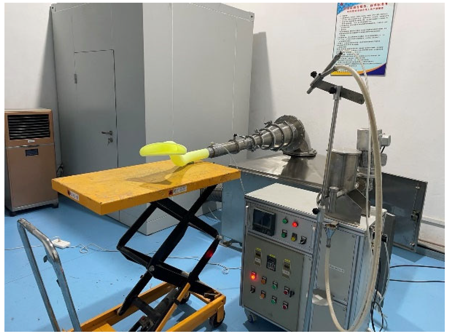
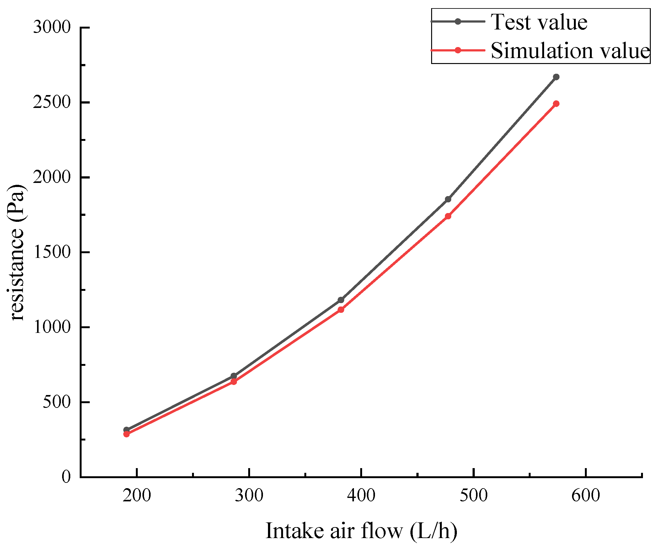
4.3. Model Flow Resistance Test of Intake Pipe

In order to verify the reliability of the numerical simulation results, the simplified model and the optimized model of the inlet dirty pipe were made into physical samples to carry out the flow–resistance test, and the simulation results were compared with the test data one by one to illustrate the reliability of the simulation results.

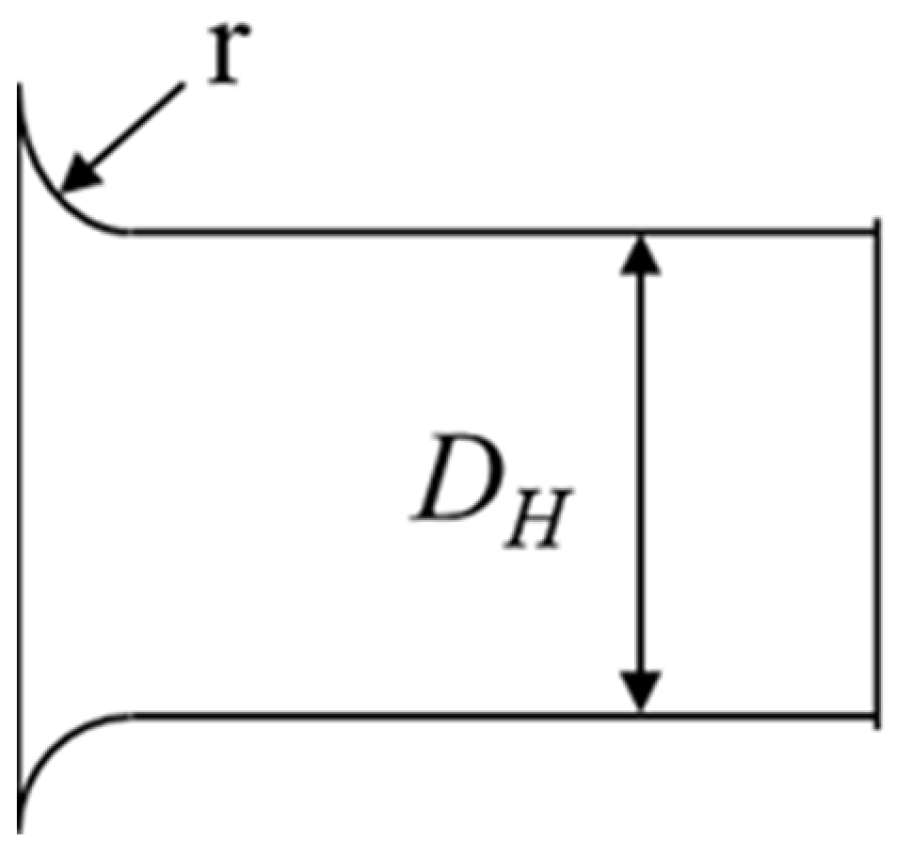
4.3.1. Test Equipment, Materials, and Methods

The sample used in this test was realized by 3D printing technology, and the material used is a high toughness resin, which has a high deformation temperature. In some high temperature areas, it can avoid deformation of the sample due to excessive temperature, which can cause significant differences between the actual object and the data model, affecting the accuracy of the test results. The finished model sample is shown in Figure 18.
The air filter pipe performance test was carried out according to the standard requirements of ISO 5011:2000. The equipment used is the JJG620-2008 air filter test bench, which was equipped with the corresponding flow resistance device. Figure 19 shows the flow resistance test device diagram.
The test method is as follows: turn on the fan switch in the reserve room, the assembly power switch, the industrial computer switch, and the computer console switch. After the ambient temperature and humidity around the test device are relatively stable, fix the tested part on the front end of the test device, open the test operation software, enter the main interface to select the percentage test, and then set its value to 50%, 75%, 100%, 125%, and 150%, according to the rated flow. Click the start test button—the test device will run automatically—and observe the relevant data changes and flow–resistance curve through the operating platform. After the test, remove the tested part, turn off all power supplies, and adjust the test console to the shutdown state. According to the above process, the optimized model sample was retested and the test data results were obtained. In order to ensure the reliability of the test data results, the method of averaging multiple tests was adopted during the flow–resistance test. The data obtained from each test were recorded and compared with the data obtained from the simulation to analyze whether there was any difference in the data.

4.3.2. Test Results and Discussion

We averaged the obtained data, as shown in Table 2. It can be seen from the table that with the increase in intake flow, the resistance gradually increases, and the overall resistance value of the optimized intake dirty pipe model is significantly lower compared to before performance improvement.
We carried out numerical simulation analysis on the optimized simplified model of the intake dirty pipe under different flow conditions, and compared the calculated results with the test values to obtain the comparison diagram of the resistance curve under different flow conditions, as shown in Figure 20.
It can be seen from Figure 20 that the outlet resistance value obtained from the actual test is higher than the resistance value obtained from the simulation. There are three main reasons for this: first, the actual measured air flow value during the test is higher than the value set during the simulation. Second, due to the influence of the ambient temperature and humidity, the test value and simulation value also have certain differences. Finally, due to the limited manufacturing technology of the sample, the inner wall surface of the pipe has an uneven surface, resulting in the high resistance measured in the actual test. In general, the difference between the simulation value and the test value is within the acceptable range, and the relevant data results obtained from the simulation are relatively reliable.
Regarding the performance improvement plan for the two structures of the intake pipe, the author believes that there is still a need for comparison compared to other scholars, such as Matsushima et al.,’s proposal to improve its pressure characteristics by increasing the diffusion angle on both sides of the pipe [34]. The author believes that this improvement method is also a good method, but for the intake pipe model mentioned in this study, increasing the curvature radius of the intake structure is equivalent to increasing the diffusion angle on both sides, and this approach is more innovative. For the scheme of increasing the bending radius at the bend of the pipeline, the author believes that this improvement method is relatively common and easy for readers to understand. Moreover, while increasing the curvature radius of the inlet structure, it can still reduce the total pressure difference between the inlet and outlet, which is also important for improving overall performance. For the two improvement methods, the author also attempted to change the optimization sequence by first increasing the bending radius at the pipeline bend. Through simulation results, it can be concluded that the total pressure difference between the inlet and outlet decreases with the increase of the bending radius, which is consistent with the conclusion obtained from optimization based on increasing the curvature radius of the inlet structure: the performance of reducing the total pressure difference by increasing the bending radius of the structure at the bending point is not significantly different from increasing the curvature radius of the inlet structure. For these two improvement methods, the author conducted a sensitivity posterior evaluation and concluded that both methods are quite important for improving performance [35]. There is no doubt that two structural improvements to the original pipeline model have a more significant improvement effect compared to improvements to a certain structure.

5. Conclusions

This research used the intake dirty pipe in the intake system of a vehicle as the main research object and carried out simulation and analysis of its internal gas flow field. The results show that there is an obvious speed mutation region at the intake and at the pipe bend, which affects the overall fluid flow uniformity and causes a pressure loss. At this time, the average total pressure difference at the inlet and outlet is 230.01 Pa. Then, the structure was optimized. The performance improvement scheme was to add a trumpet structure with a radius of 9 mm at the air inlet and adjust the bending radius at the pipe bend to 150 mm. After structural optimization, the average total pressure difference at the inlet and outlet of the pipe was 177.86 Pa, which is 22.67% lower in numerical value, and the total pressure loss was significantly reduced. The air inlet dirty pipe before and after performance improvement was made into a sample by a simplified model, and a flow–resistance test, respectively. The difference between the test data and the simulation data is within a reasonable range, and the simulation results are relatively reliable.

Author Contributions

Conceptualization, C.R. and J.L.; methodology, Z.D.; software, Z.D.; validation, Z.D.; data curation, Z.D.; writing—original draft preparation, Z.D.; project administration, J.L.; funding acquisition, J.L. All authors have read and agreed to the published version of the manuscript.

Funding

This research was funded by the National Natural Science Foundation of Hainan Province, grant number 521RC497.

Acknowledgments

Thank you to the engineers and technical experimenters from Shanghai Bindao Filter Co., Ltd., for providing me with technical exchange and support during my internship. I have received much help and effective guidance suggestions from them, which have greatly benefited me. Their professionalism and sense of responsibility for the work have aided my learning.

Conflicts of Interest

The authors declare no conflict of interest.

References

  1. Dhital, N.B.; Yang, H.-H.; Wang, L.-C.; Hsu, Y.-T.; Zhang, H.-Y.; Young, L.-H.; Lu, J.-H. VOCs emission characteristics in motorcycle exhaust with different emission control devices. Atmos. Pollut. Res. 2019, 10, 1498–1506. [Google Scholar] [CrossRef]
  2. Karthickeyan, V. Effect of combustion chamber bowl geometry modification on engine performance, combustion and emission characteristics of biodiesel fuelled diesel engine with its energy and exergy analysis. Energy 2019, 176, 830–852. [Google Scholar] [CrossRef]
  3. Khoa, N.X.; Lim, O. The effects of combustion duration on residual gas, effective release energy, engine power and engine emissions characteristics of the motorcycle engine. Appl. Energy 2019, 248, 54–63. [Google Scholar] [CrossRef]
  4. Bovendeerd, P.; Van Steenhoven, A.; Van de Vosse, F.; Vossers, G. Steady entry flow in a curved pipe. J. Fluid Mech. 1987, 177, 233–246. [Google Scholar] [CrossRef]
  5. Giannakopoulos, G.; Frouzakis, C.E.; Boulouchos, K.; Fischer, P.F.; Tomboulides, A. Direct numerical simulation of the flow in the intake pipe of an internal combustion engine. Int. J. Heat Fluid Flow 2017, 68, 257–268. [Google Scholar] [CrossRef]
  6. Sekavčnik, M.; Ogorevc, T.; Škerget, L. CFD analysis of the dynamic behaviour of a pipe system. Forsch. Ingenieurwes. 2006, 70, 139–144. [Google Scholar] [CrossRef]
  7. Ceviz, M.; Akın, M. Design of a new SI engine intake manifold with variable length plenum. Energy Convers. Manag. 2010, 51, 2239–2244. [Google Scholar] [CrossRef]
  8. Costa, R.C.; Hanriot, S.d.M.; Sodré, J.R. Influence of intake pipe length and diameter on the performance of a spark ignition engine. J. Braz. Soc. Mech. Sci. Eng. 2014, 36, 29–35. [Google Scholar] [CrossRef]
  9. Manmadhachary, A.; Kumar, M.S.; Kumar, Y.R. Design & manufacturing of spiral intake manifold to improve Volument efficiency of injection diesel engine byAM process. Mater. Today Proc. 2017, 4, 1084–1090. [Google Scholar]
  10. Sivashankar, M.; Balaji, G.; Barathraj, R.; Thanigaivelan, V. Phenomena of brake specific fuel consumption and volumetric efficiency in CI engine by modified intake runner length. In Proceedings of the IOP Conference Series: Materials Science and Engineering, Kattankulathur, India, 22–24 March 2018; IOP Publishing: Bristol, UK, 2018; p. 012086. [Google Scholar]
  11. Guo, S.; Huang, S.; Chi, M. Optimized design of engine intake manifold based on 3D scanner of reverse engineering. EURASIP J. Image Video Process. 2018, 2018, 70. [Google Scholar] [CrossRef]
  12. Jiang, F.; Li, M.; Wen, J.; Tan, Z.; Zhou, W. Optimization analysis of engine intake system based on coupling matlab-simulink with GT-power. Math. Probl. Eng. 2021, 2021, 6673612. [Google Scholar] [CrossRef]
  13. Mohamad, B.; Ali, M.Q.; Neamah, H.A.; Zelentsov, A.; Amroune, S. Fluid dynamic and acoustic optimization methodology of a formula-student race car engine exhaust system using multilevel numerical CFD models. Diagnostyka 2020, 21, 103–111. [Google Scholar] [CrossRef]
  14. Xu, P.; Jiang, H.; Zhao, X. CFD analysis of a gasoline engine exhaust pipe. J. Appl. Mech. Eng. 2016, 5, 7.1–7.7. [Google Scholar]
  15. Zhang, C.; Sun, C.; Wu, M.; Lu, K. Optimisation design of SCR mixer for improving deposit performance at low temperatures. Fuel 2019, 237, 465–474. [Google Scholar] [CrossRef]
  16. Silva, E.; Ochoa, A.; Henríquez, J. Analysis and runners length optimization of the intake manifold of a 4-cylinder spark ignition engine. Energy Convers. Manag. 2019, 188, 310–320. [Google Scholar] [CrossRef]
  17. Hanriot, S.d.M.; Queiroz, J.M.; Maia, C.B. Effects of variable-volume Helmholtz resonator on air mass flow rate of intake manifold. J. Braz. Soc. Mech. Sci. Eng. 2019, 41, 79. [Google Scholar] [CrossRef]
  18. Mezher, H.; Chalet, D.; Migaud, J.; Chesse, P. Frequency based approach for simulating pressure waves at the inlet of internal combustion engines using a parameterized model. Appl. Energy 2013, 106, 275–286. [Google Scholar] [CrossRef]
  19. Sharma, V.; Dhauni, S.; Chawla, V. Design and manufacturing of air intake assembly for formula SAE vehicle. Mater. Today Proc. 2021, 43, 58–64. [Google Scholar] [CrossRef]
  20. Mohamad, B.; Karoly, J.; Zelentsov, A.; Amroune, S. A hybrid method technique for design and optimization of Formula race car exhaust muffler. Int. Rev. Appl. Sci. Eng. 2020, 11, 174–180. [Google Scholar] [CrossRef]
  21. He, X.; Brem, B.T.; Bahk, Y.K.; Kuo, Y.-Y.; Wang, J. Effects of relative humidity and particle type on the performance and service life of automobile cabin air filters. Aerosol Sci. Technol. 2016, 50, 542–554. [Google Scholar] [CrossRef]
  22. Li, J.; Li, M.; Shen, F.; Zou, Z.; Yao, M.; Wu, C.-y. Characterization of biological aerosol exposure risks from automobile air conditioning system. Environ. Sci. Technol. 2013, 47, 10660. [Google Scholar] [CrossRef]
  23. Manikantan, R.; Gunasekaran, E.J. Modeling and analysing of air filter in air intake system in automobile engine. Adv. Mech. Eng. 2013, 5, 654396. [Google Scholar] [CrossRef]
  24. Yerram, R.; Prasad, N.; Malathkar, P.R.; Halbe, V.; Murthy, S.D. Optimization of Intake System and Filter of an Automobile Using CFD Analysis; Quality Engineering & Software Technologies (QUEST): Bangalore, India, 2006. [Google Scholar]
  25. Srinivasulu, K.; Srikanth, D.; Rafi, K.; Ramanjaneeyulu, B. Optimization of Air Filter in an Automobile Diesel Engine by Using CFD Analysis. IOSR J. Mech. Civ. Eng. 2016, 13, 78–89. [Google Scholar]
  26. HoseopSong, B.Y.; Cho, H. A study on the optimum shape of automobile air cleaner diffuser. Int. J. Appl. Eng. Res. 2017, 12, 3377–3381. [Google Scholar]
  27. Gan, H.-B.R.; Bakar, N.Z.A.; Dawood, N.F.S.; Rosli, M.A. Design improvements of an automotive air intake system. In Proceedings of the AIP Conference Proceedings, Selangor Darul Ehsan, Malaysia, 27 November 2020; p. 020008. [Google Scholar]
  28. Liu, X.; Yan, H.J.; Tian, N.; Zhao, G. CFD Simulation Analysis and Research Based on Engine Air Intake System of Automotive; SPIE: Bellingham, WA, USA, 2017; Volume 10322. [Google Scholar]
  29. Toma, M.; Stan, C.; Fileru, I. The restriction produced by the air filtration system versus the restriction produced by the air filter. MATEC Web Conf. 2018, 178, 09002. [Google Scholar] [CrossRef]
  30. Xie, J.; Liu, Z. Structural optimization on the design of an automobile engine intake pipe. J. Theor. Appl. Mech. 2022, 60, 449–461. [Google Scholar] [CrossRef]
  31. Mariotti, A.; Grozescu, A.; Buresti, G.; Salvetti, M. Separation control and efficiency improvement in a 2D diffuser by means of contoured cavities. Eur. J. Mech.-B/Fluids 2013, 41, 138–149. [Google Scholar] [CrossRef]
  32. Mariotti, A.; Buresti, G.; Salvetti, M. Use of multiple local recirculations to increase the efficiency in diffusers. Eur. J. Mech.-B/Fluids 2015, 50, 27–37. [Google Scholar] [CrossRef]
  33. Nunes, M.M.; Junior, A.C.B.; Oliveira, T.F. Systematic review of diffuser-augmented horizontal-axis turbines. Renew. Sustain. Energy Rev. 2020, 133, 110075. [Google Scholar] [CrossRef]
  34. Matsushima, T.; Takagi, S.; Muroyama, S. Characteristics of a highly efficient propeller type small wind turbine with a diffuser. Renew. Energy 2006, 31, 1343–1354. [Google Scholar] [CrossRef]
  35. Sobol, I.M. Global sensitivity indices for nonlinear mathematical models and their Monte Carlo estimates. Math. Comput. Simul. 2001, 55, 271–280. [Google Scholar] [CrossRef]
Figure 1. Three-dimensional model diagram of air filter assembly and intake pipe. It mainly consists of a: (1) intake dirty pipe, (2) resonance cavity, (3) air filter, and (4) intake clean pipe.
Applsci 13 06505 g001
Figure 2. Simplified model of air filter intake dirty pipe.
Applsci 13 06505 g002
Figure 3. Mesh model of fluid domain of air intake dirty pipe.
Applsci 13 06505 g003
Figure 4. The inlet and outlet of the model. The blue arrow represents the inlet, and the red arrow represents the outlet.
Applsci 13 06505 g004
Figure 5. y = 0 mm, xoz section velocity contour.
Applsci 13 06505 g005
Figure 6. z = −106 mm, xoy section velocity contour.
Applsci 13 06505 g006
Figure 7. z = 0 mm, xoy section velocity vector.
Applsci 13 06505 g007
Figure 8. y = 0 mm, xoz section pressure contour (before performance improvement).
Applsci 13 06505 g008
Figure 9. z = −106 mm, xoy section pressure contour (before performance improvement).
Applsci 13 06505 g009
Figure 10. Schematic diagram of air inlet structure optimization.
Applsci 13 06505 g010
Figure 11. z = 0 mm, velocity vector at different radius inlet structures of the xoy section. (a) Horn-shaped radius is 3 mm. (b) Horn-shaped radius is 5 mm. (c) Horn-shaped radius is 7 mm. (d) Horn-shaped radius is 9 mm. (e) Horn-shaped radius is 11 mm. (f) Horn-shaped radius is 13 mm. (g) Horn-shaped radius is 15 mm.
Applsci 13 06505 g011
Figure 12. Relationship between total pressure difference in inlet and outlet under the radius change in trumpet structure.
Applsci 13 06505 g012
Figure 13. y = 0 mm; velocity contour at different bending radii of xoz section. (a) Bending radius is 60 mm. (b) Bending radius is 90 mm. (c) Bending radius is 120 mm. (d) Bending radius is 150 mm. (e) Bending radius is 180 mm.
Applsci 13 06505 g013
Figure 14. z = −106 mm; velocity contour at different bending radii of xoy section. (a) Bending radius is 60 mm. (b) Bending radius is 90 mm. (c) Bending radius is 120 mm. (d) Bending radius is 150 mm. (e) Bending radius is 180 mm.
Applsci 13 06505 g014aApplsci 13 06505 g014b
Figure 15. Relationship between the total pressure difference between inlet and outlet with bending radius.
Applsci 13 06505 g015
Figure 16. y = 0 mm, xoz section pressure contour (after performance improvement).
Applsci 13 06505 g016
Figure 17. z = −106 mm, xoy section pressure contour (after performance improvement).
Applsci 13 06505 g017
Figure 18. Simplified sample model of intake dirty pipe. The upper part is the sample after performance improvement, and the lower part is the sample before performance improvement.
Applsci 13 06505 g018
Figure 19. Flow resistance test device. The test piece is installed on a flow resistance device for testing.
Applsci 13 06505 g019
Figure 20. Comparison of test and simulation value.
Applsci 13 06505 g020
Table 1. Setting parameters of boundary conditions of inlet dirty pipe model.
AreaBoundary TypeBoundary Condition
InletPressure inletTotal pressure is 0 Pa,
turbulence intensity is 4.11%, hydraulic diameter is 76 mm
OutletMass flow outletMass flow rate is 0.1227555 kg/s
Table 2. Pre- and post-performance improvement test values under average processing.
Model before Performance ImprovementModel after Performance Improvement
Intake Air Flow (L/h)Average Resistance (Pa)Intake Air Flow (L/h)Average Resistance (Pa)
190.93314.66190.81287.12
286.62674.58286.38637.04
382.131181.72381.831117.14
477.681853.51477.361741.26
574.142670.29573.752491.76
Disclaimer/Publisher’s Note: The statements, opinions and data contained in all publications are solely those of the individual author(s) and contributor(s) and not of MDPI and/or the editor(s). MDPI and/or the editor(s) disclaim responsibility for any injury to people or property resulting from any ideas, methods, instructions or products referred to in the content.

