Structural Analysis and Optimization of Urban Gas Pressure Regulator Based on Thermo-Hydro-Mechanical Coupling

Abstract

As a core component in the gas transmission process, the internal wall surface of a gas pressure regulator is prone to failure due to long-term exposure to a high-pressure gas environment, resulting in poor reliability of the regulator. Thus, a thermo-hydro-mechanical coupling model for the FL gas pressure regulator is established in this paper, and the thermo-hydro-mechanical coupling results are verified by engineering data. The effect of valve opening on the parameters (temperature, deformation, and stress) of the gas pressure regulator is studied in detail through simulation. The results show that the stress is greater at the sleeve, valve bore, and outlet valve seat wall under the opening of 20% of the regulator. Finally, the response surface method is used to optimize the regulator to obtain a good fit and high predictive ability of the response surface equation. The optimal parameters for the gas pressure regulator are as follows: the wall thickness of the sleeve is 7.25 mm, the diameter of the valve bore is 25 mm, and the wall thickness of the outlet seat is 31.05 mm. The maximum equivalent stress with this combination of parameters is 135.62 MPa.

1. Introduction

The gas pressure regulator is one of the key facilities of a gas station and is a core component in the gas transmission process. The main function is to adjust the higher gas inlet pressure to set a lower gas outlet pressure and to automatically keep the outlet pressure value within a certain range as the gas consumption changes and the inlet pressure fluctuates. The gas pressure regulator is one of the most vulnerable parts at the gas field station, and thus, it has been selected as the research object for relevant research.

Several scholars from related fields have explored gas pressure regulator failure problems and achieved important results. Ramzan et al. [1] developed a regulator model and conducted simulations of the regulator flow field. Zhi et al. [2,3] used support vector machines to diagnose regulator faults. Toyoda et al. [4] developed a compact, portable detection system that detects diaphragm vibrations to determine whether a regulator is malfunctioning. In recent years, with the continuous development and improvement of simulation technology, the thermo-hydro-mechanical coupling simulation method has been widely used in various disciplines. Lee et al. [5] investigated the applicability of FLAC 3D in reproducing the coupled thermal-hydro-mechanical (THM) behavior of Opalinus clay. Partoaa et al. [6] investigated the effect of audit sheet attachment on the thermal stress reduction in off-road diesel engines based on the thermo-hydrodynamic-solid coupling method. Nariman [7] investigated the effect of transient and steady-state heat transfer on fire-induced eddy-excited vibration and fatigue in segmental bridge decks using coupled heat flow in solids and coupled heat-stress analysis methods. The response surface method is another common mechanical structure optimization design method. For example, Mahtab et al. [8] statistically evaluated the effectiveness of advanced oxidation technology for waste leachate treatment using response surface methodology based on fenton and determined the optimal operating conditions. Sarikaya et al. [9] analyzed the machining parameters of CNC turning based on the response surface method. Karimifard et al. [10] applied response surface methodology to remove dyes physicochemically from wastewater. Meanwhile, Sarafraz et al. [11] conducted smart optimization of thermosyphon heat pipes for evacuated tube solar collectors using response surface methodology. Based on previous studies, using the THM coupling method in the structural analysis of gas pressure regulators and optimizing the structure of pressure regulators by the response surface method is extremely rare. Therefore, this paper will also use the response surface method to optimize the structure of a voltage regulator based on the results of the THM coupling analysis.

2. Theoretical Model

The THM coupling problem involves the interaction between the temperature, flow, and solid deformation fields. The coupling effect between fields works through interface forces. The coupling solution is achieved through one-way coupling using two field-cross iterations [12].

• Continuity equation

The conservation of mass in fluid flow is expressed through continuity equations:

$$\frac{\partial \rho }{\partial t}+\frac{\partial (\rho u_x)}{\partial x}+\frac{\partial (\rho u_y)}{\partial y}+\frac{\partial (\rho u_z)}{\partial z}=0$$

(1)

where $u_x$, $u_y$ and $u_z$ represent the velocity components in three directions, t is time, and ρ is the density.

• Momentum equation

For a given fluid element, the momentum change rate over time is equal to the sum of various external forces acting on the element.

$$\frac{\partial (\rho u_x)}{\partial t}+\nabla •(\rho u_x\overrightarrow{u})=-\frac{\partial p}{\partial x}+\frac{\partial {\tau }_{xx}}{\partial x}+\frac{\partial {\tau }_{yx}}{\partial y}+\frac{\partial {\tau }_{zx}}{\partial z}+\rho f_x$$

(2)

$$\frac{\partial (\rho u_y)}{\partial t}+\nabla •(\rho u_y\overrightarrow{u})=-\frac{\partial p}{\partial y}+\frac{\partial {\tau }_{xy}}{\partial x}+\frac{\partial {\tau }_{yy}}{\partial y}+\frac{\partial {\tau }_{zy}}{\partial z}+\rho f_y$$

(3)

$$\frac{\partial (\rho u_z)}{\partial t}+\nabla •(\rho u_z\overrightarrow{u})=-\frac{\partial p}{\partial z}+\frac{\partial {\tau }_{xz}}{\partial x}+\frac{\partial {\tau }_{yz}}{\partial y}+\frac{\partial {\tau }_{zz}}{\partial z}+\rho f_z$$

(4)

where ρ is the pressure on the fluid element, ${\tau }_{xx}$, ${\tau }_{xy}$ and ${\tau }_{xz}$ are the components of viscous stress on the surface of a microelement caused by molecular viscosity, and $f_x$, $f_y$ and $f_z$ are the unit mass forces in three directions.

• Energy equation

$$\frac{\partial (\rho E)}{\partial t}+\nabla •[\overrightarrow{u}(\rho E+p)]=\nabla •[k_{eff}\nabla T-{\displaystyle \sum _j{h}_j{J}_j}+({\tau }_{eff}•\overrightarrow{u})]+S_h$$

(5)

$$E=h-p/\rho +u^2/2$$

(6)

where E is the total energy of the fluid micro cluster, $h$ is enthalpy, $h_{eff}$ is the enthalpy of component j, $k_{eff}=k+k_t$, $k_t$ is the effective thermal conductivity coefficient, $J_j$ is the diffusion flux of component $j$, and $S_h$ includes chemical reaction heat and other user-defined volumetric heat source terms.

• Discrete solid structure’s equation of motion

The solid structure motion equation can be described as follows:

$$M_{\mathrm{s}}\ddot{r}+C_{\mathrm{s}}r+K_{\mathrm{s}}r+f_{\mathrm{p}}+f_0=0$$

(7)

where M_s is the displacement mass matrix of the structure, C_s is the damping matrix of the structure, K_s is the stiffness matrix of the structure, $f_{\mathrm{p}}$ is the nodal vector of fluid at the fluid-structure interface of the strike plate, and $f_0$ is the vector of the external motivator.

• Heat transfer control equation

$$Q=kA\Delta t_m$$

(8)

where k is the heat transfer coefficient, A is the heat transfer area, and $\Delta t_m$ is the average temperature difference for heat transfer [13].

Numerical calculations are conducted in the fluid domain of the gas regulator. The temperature load and flow field of the fluid–solid boundary calculated in the fluid domain are loaded onto the corresponding fluid–solid interface of the gas regulator. The temperature and heat flux fields on the inner wall of the gas regulator are also calculated. Then, the temperature field and thermal stress in the solid domain are calculated, and the final coupling analysis of the calculation results in the fluid and solid domains is conducted to obtain the deformation and stress situation of the overall structure of the gas pressure regulator.

3. Calculation Model for the Gas Pressure Regulator

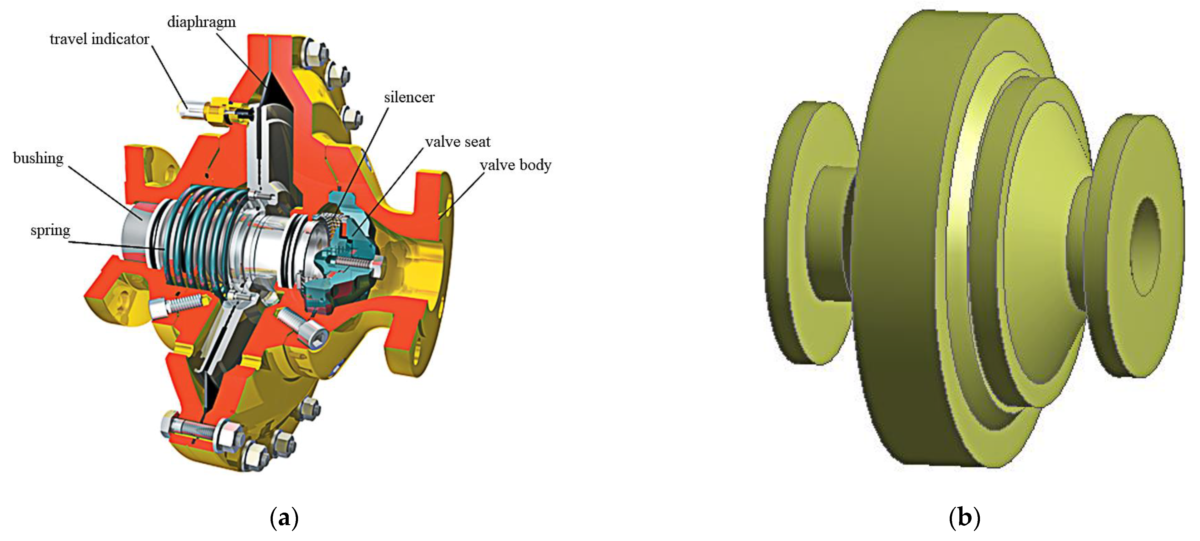
3.1. Geometric Model

This paper takes the widely used FL series gas pressure regulator as the research object, and the schematic diagram of the structure is shown in Figure 1a. The valve spool is integrated with the membrane through the left and right pallets. The spring acts on the left pallet, enabling the diaphragm to drive the sleeve to move left and right. When the regulator works, the conductor will apply pressure before and after the valve to the chambers at the left and right ends of the diaphragm for comparison according to the pressure requirement. The force on the higher-pressure side will deform the diaphragm and move to the lower-pressure side, causing the spring to drive the sleeve together. Considering the complex structure of the FL series gas pressure regulator (Figure 1a), a simplified calculation model for the regulator is established (Figure 1b).

Due to the limitations of the simulation and the complexity of gas motion and gas composition, the following assumptions are proposed: (1) the gas composition is only methane; (2) the flow state is turbulent based on the k-ε turbulence model; (3) the fluid has a uniform temperature distribution before flowing through the regulator; and (4) the regulator has no heat loss.

3.2. Thermo-Hydro-Mechanical Coupling Model

The thermo-hydro-mechanical coupling problem involves the interaction among the fields (flow, pressure, temperature, structure deformation, etc.). In this paper, the one-way coupling method is chosen to solve the structure of the regulator, and the basic control equations should be satisfied in the solution process [14].

The main parameters are set in the fluid domain as follows: (1) the specific pressure values of the pressure inlet and outlet are set according to

Table 1. Comparison between the operation data and simulation data.

Number	Inlet Pressure (MPa)	Outlet Pressure (MPa)	Outlet Wall Temperature (°C)	Outlet Flow (m³/h)	Simulation of Wall Surface Temperature (°C)	Simulation of Outlet Flow (m³/h)	Relative Error of Wall Surface Temperature (%)	Flow Relative Error (%)
1	2.93	1.31	19.9	83,706.98	20.8	77,328.51	4.52	7.60
2	2.93	1.39	20.5	85,942.66	19.8	79,631.89	3.41	7.34
3	2.91	1.37	20.5	85,451.60	19.8	81,842.12	3.41	4.22
4	2.93	1.69	21.5	97,148.79	20.3	87,761.30	5.58	9.66
5	2.92	1.89	22.1	100,777.39	21.6	95,421.00	2.26	5.32
6	2.92	1.56	20.9	94,991.37	19.7	84,284.89	5.74	11.27
7	2.92	1.33	20.1	84,525.12	19.2	77,397.96	4.48	8.43
8	2.91	1.46	21.4	93,508.88	20.3	87,475.69	5.14	6.45
9	2.92	1.61	22.8	96,564.26	21.8	92,912.20	4.39	3.78
10	2.93	1.47	20.7	93,557.04	19.0	87,399.12	8.21	6.58
11	2.93	1.71	21.8	98,164.84	20.9	93,872.09	4.40	4.37

; (2) the turbulent flow is selected, and the standard k-ε model is used; (3) the wall surface is set as a standard wall function; (4) the gravitational acceleration value is 9.81 m/s², and the direction is z-axis positive; (5) the hydraulic diameter is 0.2 m, and the turbulence intensity is 5%; and (6) the gas temperature is 20 °C.

The main parameters are set in the structure domain: (1) the ambient temperature is 22 °C; (2) the material is selected as steel; and (3) the fixing surface is on the end face of the inlet and outlet of the regulator and the middle circular curved surface.

Meanwhile, the mesh size of the fluid domain contact surface is 1 mm, the expansion layer is set to five layers, and the tetrahedral mesh is used to divide the mesh size by 3 mm. The mesh size of the structure domain contact surface is set to 3 mm, the rest of the solid part is set to 5 mm, and the tetrahedral mesh is used to divide the mesh, as shown in Figure 2.

4. Model Validation

In this paper, the model is somewhat simplified in numerical calculation, and some conditions are idealized; therefore, the model must be validated. Conducting relevant tests is not feasible because of the high gas pressure inside the gas regulator, complex flow conditions, and dangerous environmental conditions. Thus, the engineering verification method is chosen in this paper. The simulation results are compared and analyzed with the on-site operation data.

Eleven sets of operating data from a gas field station are selected for simulation analysis, and the comparison between the operating data and simulation results is shown in Table 1.

The relative error rate of the wall temperature at the outlet between the engineering and the simulation results is 8.21%, and the average error rate is 4.69%. The relative error rate of the flow rate at the outlet is up to 11.27%, and the average error rate is 6.82%. The simulation results are similar to the actual results, the error rate is acceptable, and the established regulator model is reliable [15].

5. Simulation Results and Analysis

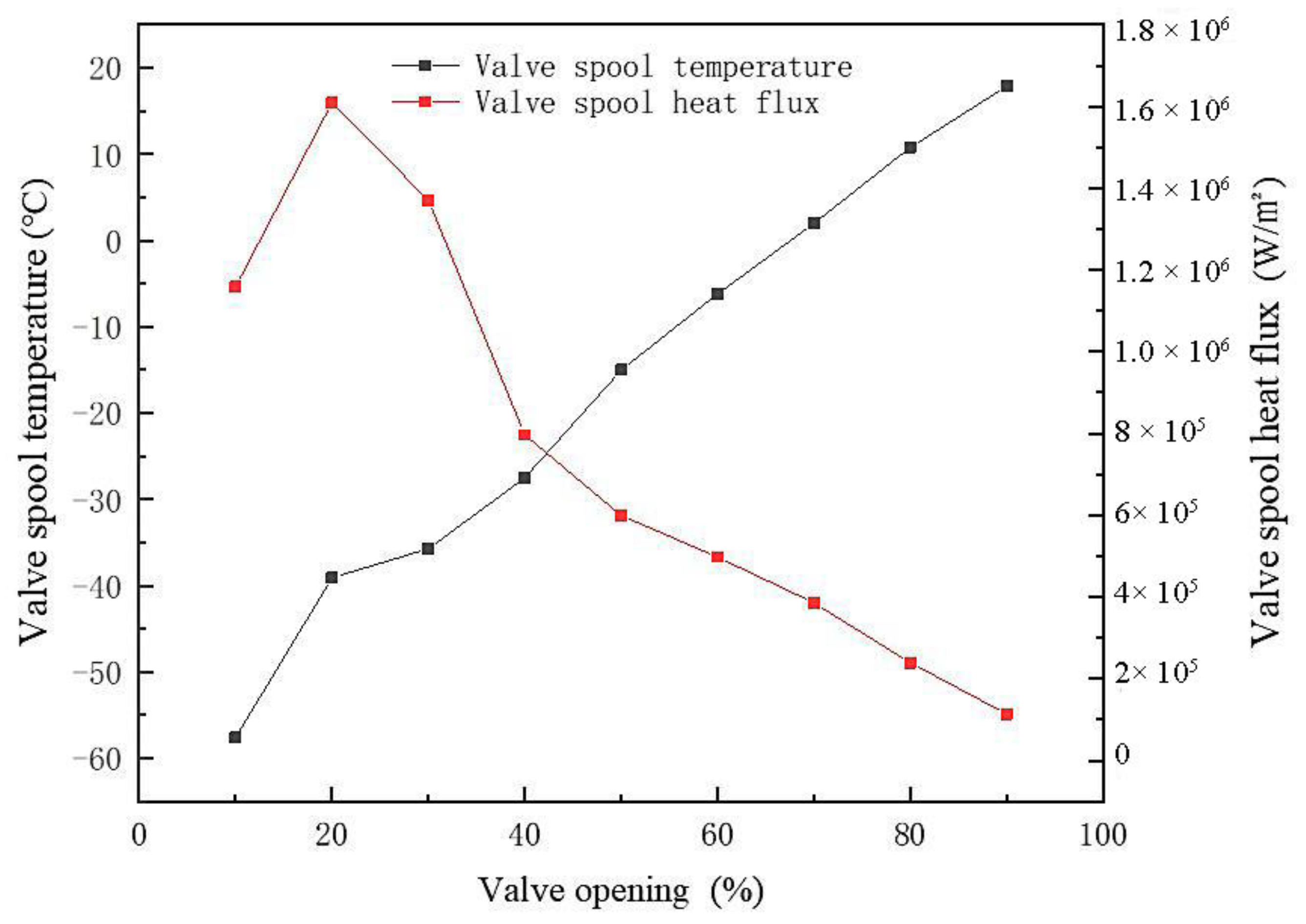
5.1. Temperature Field and Heat Flux Analysis

A large temperature difference between the inlet and outlet can be observed in the gas pressure regulator during the operation process, adversely affecting the normal operation of the regulator and the regulator structure during long-term operations. When the valve opening is small, the working conditions for the gas pressure regulator are more severe, and the overall structure will be subject to greater stress and strain. The analysis of the temperature field and heat flux for the gas pressure regulator provides an important reference for the subsequent study of the stress and deformation and the determination of the optimization parameters.

Based on the THM coupling theory, gas pressure regulator models with nine openings (10% to 90%) were simulated. The temperature field and heat flux results for the model with a 50% opening are shown as an example in Figure 3. When the opening is 50%, the regulator has a large temperature drop on the wall at the valve spool, and the temperature in some areas drops below 0 °C. At the same time, the heat flux increased significantly at the outlet spool position, and a large amount of heat exchange can be observed at the outlet spool position, which is derived mainly from the heat lost when the gas flows through the part.

To visualize the trend of temperature field and heat flux at the outlet spool position for the gas pressure regulator, the operating conditions, including nine openings (from 10% to 90%), are summarized in Figure 4. The figure shows that under the small valve opening, the temperature at the outlet spool is very low. Some areas even reach −50 °C or less. At the same time, the heat flux is also high, indicating that when the valve opening is small, a large heat exchange can be observed at the spool position, and the working condition is more severe. As the valve opening increases, the temperature at the outlet spool rises, the heat flux decreases, and the operating condition improves. Therefore, the THM coupling effect should be considered in the analysis of the regulator structure.

5.2. Deformation and Stress Analysis

Various factors (such as temperature, inlet pressure, impurities, etc.) may cause a certain amount of deformation in the gas pressure regulator as a whole or in part of the structure. A large deformation can affect the overall performance of the regulator, leading to failure in serious cases. At the same time, the deformation of the regulator is affected by the stress because the long-term work under high pressure and high flow rate gas conditions will cause its internal flow channel to be subjected to different degrees of cavitation.

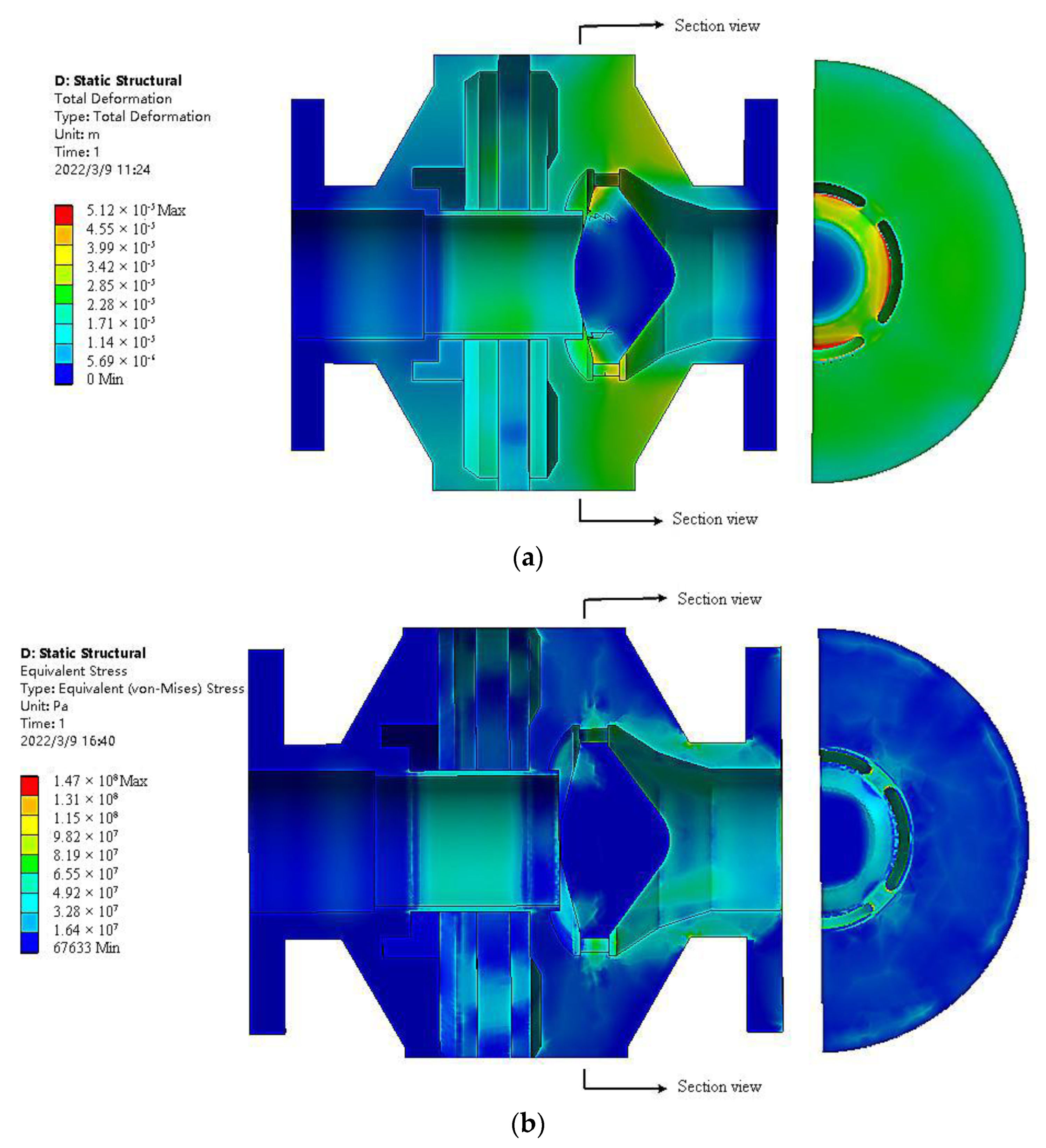
5.2.1. Total Deformation

The THM coupling simulations are carried out for the gas pressure regulator with nine openings to analyze the total deformation at each opening. Figure 5 illustrates the result for the regulator at 50% opening. Figure 5a shows a larger deformation at the sleeve, valve bore, and outlet valve seat wall for the regulator. Figure 6 shows the deformation at the three regulator locations under the nine openings.

Figure 6 shows that the maximum deformation of the regulator sleeve, valve hole, and outlet seat wall appears at the 20% opening. At the same time, with the increase in the opening, the wall deformation at the valve hole and outlet seat is gradually reduced, and the sleeve deformation has a fluctuating downward trend. The deformation is relatively small at the 10% opening due to the smaller opening’s structural stiffness. Compared to other parts, although the largest deformation occurs at the sleeve, valve bore, and outlet valve seat wall, from an overall perspective, the total deformation is still at a low level, and thus, the normal operation of the regulator is less affected.

5.2.2. Equivalent Stress

The equivalent stress of the overall structure of the regulator with 50% opening is compared in Figure 5b. It shows that the stress in the regulator sleeve, valve bore, and export valve seat wall is relatively large. The gas regulator under different degrees of opening and the equivalent stress on each part of the statistics are drawn into the relevant curve shown in Figure 7 to intuitively understand the regulator of the main stress parts of the stress trends.

Figure 7 shows that when the valve opening is small, the regulator is subjected to large stresses at the sleeve, valve opening, and outlet seat wall. At the same time, as the valve opening increases, the stress on each part decreases significantly. When the opening is 20%, the working conditions of the regulator are more complex, and the sleeve and the outlet valve seat wall stress have a certain rise. The stress at the valve bore has not shown a significant decline. When the opening is greater than 50%, the stress on the regulator parts decreases significantly and is maintained at 150 MPa. Meanwhile, the regulator’s operating conditions have improved.

Considering the above factors, the thermo-hydro-mechanical coupling model of the gas pressure regulator with a 20% opening is selected as the optimization object in this paper.

6. Regulator Structure Optimization Analysis

Based on the experimental data obtained from the response surface method, the influence of parameters such as sleeve wall thickness, valve orifice diameter, and outlet seat wall thickness on the displacement and equivalent stress of the gas pressure regulator is also considered. The sleeve wall thickness, valve bore diameter, and outlet valve seat wall thickness are selected as the optimization parameters. The equivalent effect stress is chosen as the optimization objective function to optimize the design of the regulator structure.

Table 2. Constraints on the design parameters of the gas pressure regulator.

Parameters	Variables	Constraint Conditions
Sleeve wall thickness	x1	4.5 mm ≤ x1 ≤ 10 mm
Valve hole diameter	x2	20 mm ≤ x2 ≤ 30 mm
Outlet valve seat wall thickness	x3	27 mm ≤ x3 ≤ 35 mm
Equivalent force	Y	Y ≥ 0

shows the relevant design requirements of the gas pressure regulator [14] and the formal variables and solution range of relevant parameters.

6.1. Optimization Scheme Design

This optimization design aims to find the minimum equivalent stress value by satisfying the parameters of sleeve wall thickness, valve port diameter, and outlet seat wall thickness. The formal variables and solution ranges of the parameters are determined by checking the relevant design requirements for the gas pressure regulators and considering the economic benefits, as shown in Table 2.

For the optimal design of the three factors, a binary nonlinear fit is adopted in this paper, and the objective function is chosen as a quadratic function.

$$Y_{}=a_0+a_1{x}_1+a_2{x}_2+a_3{x}_3+a_4{x}_1{x}_2+a_5{x}_1{x}_3+a_6{x}_2{x}_3+a_7{x}_1^2+a_8{x}_2^2+a_9{x}_3^2$$

(9)

The design principle of the response surface method is used to obtain 17 sets of experimental parameters. Then, 17 regulator models are established for the simulation calculations. The experimental parameters and corresponding equivalent stresses are shown in

Table 3. Test schemes and corresponding response values of the gas pressure regulator.

Number	Number of Calculations (Times)	Sleeve Wall Thickness (mm)	Valve Hole Diameter (mm)	Outlet Valve Seat Wall Thickness (mm)	Equivalent Stress (MPa)
1	6	7.25	25	27.1	175.8
2	13	7.25	25	31.05	181.85
3	15	7.25	25	31.05	185.62
4	17	7.25	25	31.05	179.42
5	8	7.25	25	35	204.69
6	12	7.25	30	35	185.23
7	3	7.25	30	31.05	202.16
8	11	7.25	20	35	198.57
9	2	7.25	20	31.05	178.85
10	5	10	25	27.1	175.97
11	16	10	25	31.05	187.38
12	1	10	20	31.05	198.47
13	10	10	30	27.1	172.95
14	14	4.5	25	31.05	217.96
15	7	4.5	25	35	145.33
16	4	4.5	30	31.05	241.47
17	9	4.5	20	27.1	171.64

.

6.2. Analysis of Optimization Results

The coefficients of the response surface model are shown in

Table 4. Response surface model coefficients.

Parameters	Regression Coefficient	Degree of Freedom	Standard Error	95% CI Lower Bound	95% CI Upper Bound
intercept distance	204.94	1	8.72	184.32	225.56
x1	−5.02	1	6.90	−8.32	−1.71
x2	−3.20	1	6.90	−4.51	−1.90
x3	19.90	1	6.90	3.60	36.21
x1 x2	2.18	1	9.75	0.13	4.24
x1 x3	7.48	1	9.75	1.43	13.54
x2 x3	13.87	1	9.75	0.81	26.93
$x_1^2$	−10.68	1	9.50	−13.16	−8.21
$x_2^2$	−17.62	1	9.50	−30.09	−5.14
$x_3^2$	−13.03	1	9.50	−23	−3.06

and indicate a 95% confidence interval for each parameter. This interval can be used to determine the significance of each parameter. If the upper and lower bounds of the interval do not contain 0, then the term is significant. If it contains 0, the term is insignificant, and the corresponding parameter should be excluded. Whether the exclusion is determined will be further judged according to the analysis of variance (ANOVA).

After obtaining the relationship between input variables, response values, and variables, the significance test of the regression using ANOVA is conducted to determine the significance of each item (

Table 5. Analysis of variance.

Source of Variation	Sum of Squares	Degree of Freedom	Mean SQUARE	$\mathit{F}$	p Value	Significance
Models	7243.12	9	804.79	48.33	<0.0001	***
$x_1$	201.40	1	201.40	11.35	0.0028	**
$x_2$	82.11	1	82.11	178.31	<0.0001	***
$x_3$	3168.48	1	3168.48	26.77	<0.0001	***
x1 x2	19.05	1	19.05	93.43	<0.0001	***
x1 x3	223.95	1	223.95	9.12	0.0143	*
x2 x3	769.51	1	769.51	112.47	<0.0001	***
$x_1^2$	480.49	1	480.49	8.44	0.011	*
$x_2^2$	1306.48	1	1306.48	17.91	0.0044	**
$x_3^2$	714.87	1	714.87	13.29	0.0015	**
Residuals	2662.31	7	380.33
Pure Error	0	4	0.00
Total	9905.42	16

Note: *** is very significant; ** is significant; * is less significant.

). The value of F indicates the significance of the whole fitted equation, and the larger the F, the more significant the equation and the better it fits. However, to determine the significance of the variables, the value of p must be analyzed. The p of the regression model measures the magnitude of the difference between the control and experimental groups. If p is less than 0.0001, it indicates that the choice of the quadratic polynomial for the response surface model is very reasonable and that the relationship between the regression equation and the equivalent stresses is significant. It also indicates that the presence of variables has a positive effect on the significance of the model.

The regulator model is analyzed to verify the applicability of the model using a residual-based diagnostic plot obtained from regression analysis methods. A normal probability plot is considered the ideal normal probability if the reference points are distributed along a straight line. Figure 8 shows the residual normal probability plot, which shows that the reference points are uniformly distributed on both sides of the straight line. Although individual reference points can be observed with the offset, the impact on the model is not significant or acceptable. Hence, the data for calculating the results of the equivalent stress in this paper are accurate and meet the requirements.

Figure 9 shows the residuals versus the number of trials plot and the predicted value plot, which can be used to check the reasonableness of the model. The plot indicates that all residuals are distributed within the horizontal band between the two red lines, which means that the quadratic polynomial model is reasonable.

Table 6. Summary of predicted and actual values.

Number of Tests	Actual Value (MPa)	Predicted Value (MPa)	Relative Error (%)
6	135.62	137.32	1.24
15	145.33	148.83	2.35
3	171.64	171.47	0.01
5	172.95	176.27	1.88
8	175.80	170.60	2.96
16	175.97	172.65	1.89
10	178.85	173.83	2.81
11	179.42	204.94	12.45
2	181.85	187.05	2.78
1	185.23	183.53	0.92
9	187.38	204.94	9.37
14	198.47	204.94	3.16
4	198.57	203.59	2.47
12	202.16	198.66	1.73
17	204.69	204.86	0.08
13	217.96	204.94	5.97
7	241.47	204.94	15.13

shows the comparison between the predicted and actual values. The maximum relative error is 15.13%, indicating that the predicted and actual values have a good correlation and that the quality of prediction and the accuracy of the model are high.

The regression diagram can visualize the trend of each variable, and the change of the equivalent stress can also be visualized. The change in the slope of each curve shows how sensitive the equivalent stress is to each variable.

Figure 10 shows that the equivalent stress increases with the sleeve wall thickness and the diameter of the valve bore, and then the value decreases. This result indicates that increasing the above values is beneficial for reducing the equivalent force. Equivalent stress with the increase in wall thickness of the outlet seat has a certain upward trend, but the rising trend gradually slows down, negatively affecting the reduction of the equivalent force. Hence, larger is not necessarily better in selecting the outlet seat wall thickness; rather, it should be taken within a reasonable range of values.

The three-dimensional response surface plot can more intuitively show the effect of the two variables acting simultaneously on the equivalent force. The two-dimensional contour plot can represent the mutually changing relationship between the two variables. Therefore, the three-dimensional response surface diagram and its two-dimensional contour diagram are shown in Figure 11.

The gas regulator secondary response surface interaction term surface image and the corresponding contour plot can be analyzed under the simultaneous action of the two factors equivalent effect force change law. As the sleeve wall thickness and valve hole diameter increase, the equivalent effect force first increases and then decreases. When the outlet seat wall thickness is small, the sleeve thickness and valve hole diameter increase, and the equivalent effect force decreases significantly. The above results are consistent with the results of the regenerative analysis.

The above diagnostic analysis, regression analysis, and ANOVA can obtain response surface equations with good fit and high predictive ability, and the response surface’s fitting coefficients are substituted into the objective optimization function (Equation (9)). Thus, the optimization function for the gas pressure regulator can be obtained.

$$Y=204.94-5.02x_1-3.20x_2+19.90x_3+2.18x_1{x}_2+7.48x_1{x}_3+13.87x_2{x}_3-10.68x_1^2-17.62x_2^2-13.03x_3^2$$

(10)

The extreme value of the response surface is the optimal parameter. The optimal parameters of the gas regulator can be obtained according to the surface and optimization function analyses. The sleeve wall thickness is 7.25 mm, the valve hole diameter is 25 mm, the outlet valve seat wall thickness is 31.05 mm, and the equivalent stress is 135.62 MPa.

All the above parameters are within the constraints specified in Table 2. A comparison of the equivalent stress in Figure 9 shows that at the 20% opening, the equivalent stress after optimization is significantly lower than the equivalent stress before optimization, and this optimization scheme has high feasibility. Through this method, the pressure use requirements of the regulator can be met while reducing the equivalent stress and improving the reliability of the structure through the optimization of the key structural dimensions of the regulator.

7. Conclusions

(1)

Based on the thermal analysis of the gas regulator, temperature and heat flux in the regulator operation process have obvious fluctuations in the regulator structure. The effect of temperature and heat flux on the regulator should be considered during the simulation.

(2)

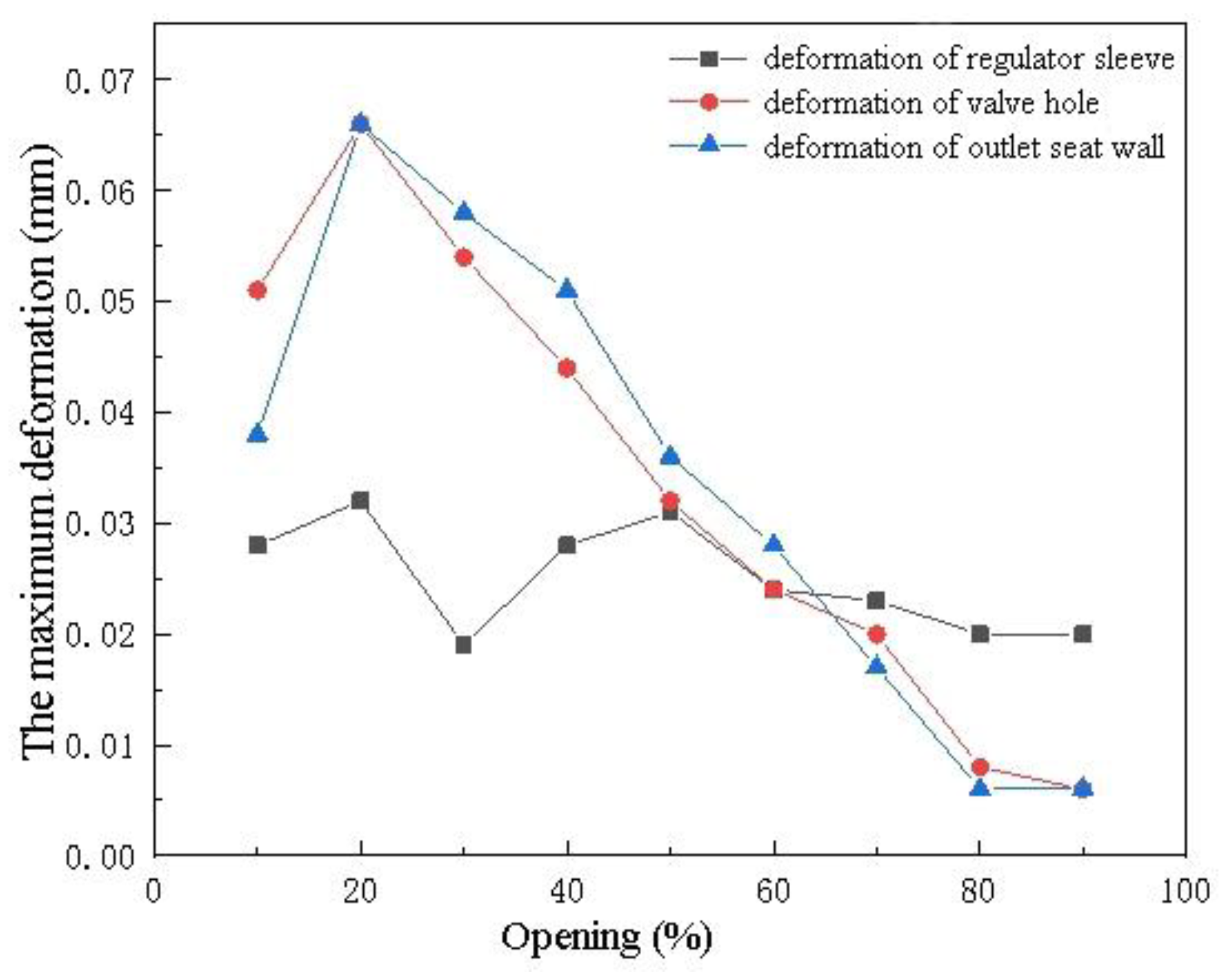
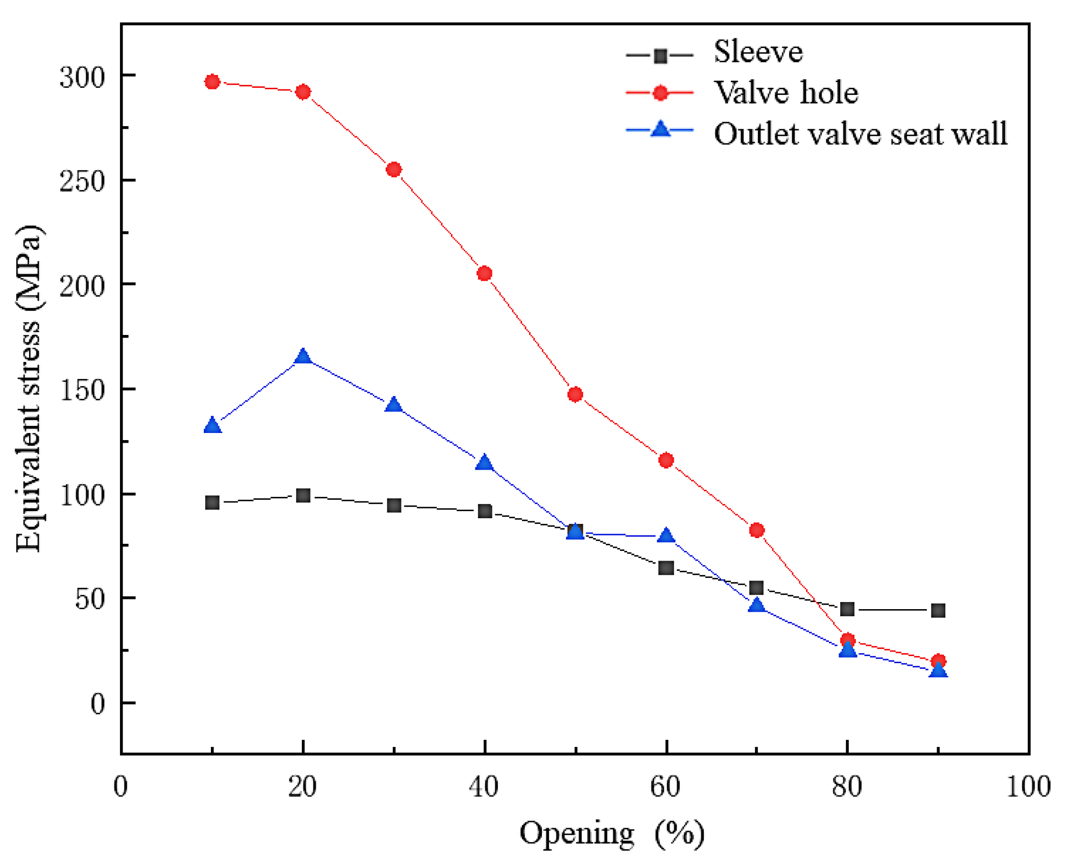
According to the thermo-hydro-mechanical analysis of the gas regulator, the maximum deformation of the regulator sleeve, valve bore, and outlet valve seat wall occurs when the opening is 20%, and the maximum deformation of each part is 0.032 mm, 0.066 mm, and 0.066 mm, respectively. At the same time, as the opening increases, the deformations of the regulator valve hole and outlet seat wall gradually decrease, and the sleeve deformation tends to fluctuate. When the valve opening is small, the sleeve, valve, and outlet seat wall regulator are subject to greater stress. The maximum stress on each part is 98.9 MPa, 292.1 MPa, and 164.9 MPa, respectively. At the same time, with the increase in the opening of the valve port, the stress on each part decreases significantly. At 20% opening, the working conditions of the regulator are complex; the stress on the sleeve and outlet valve seat wall has a certain rise, and the stress on the valve bore has no significant decrease.

(3)

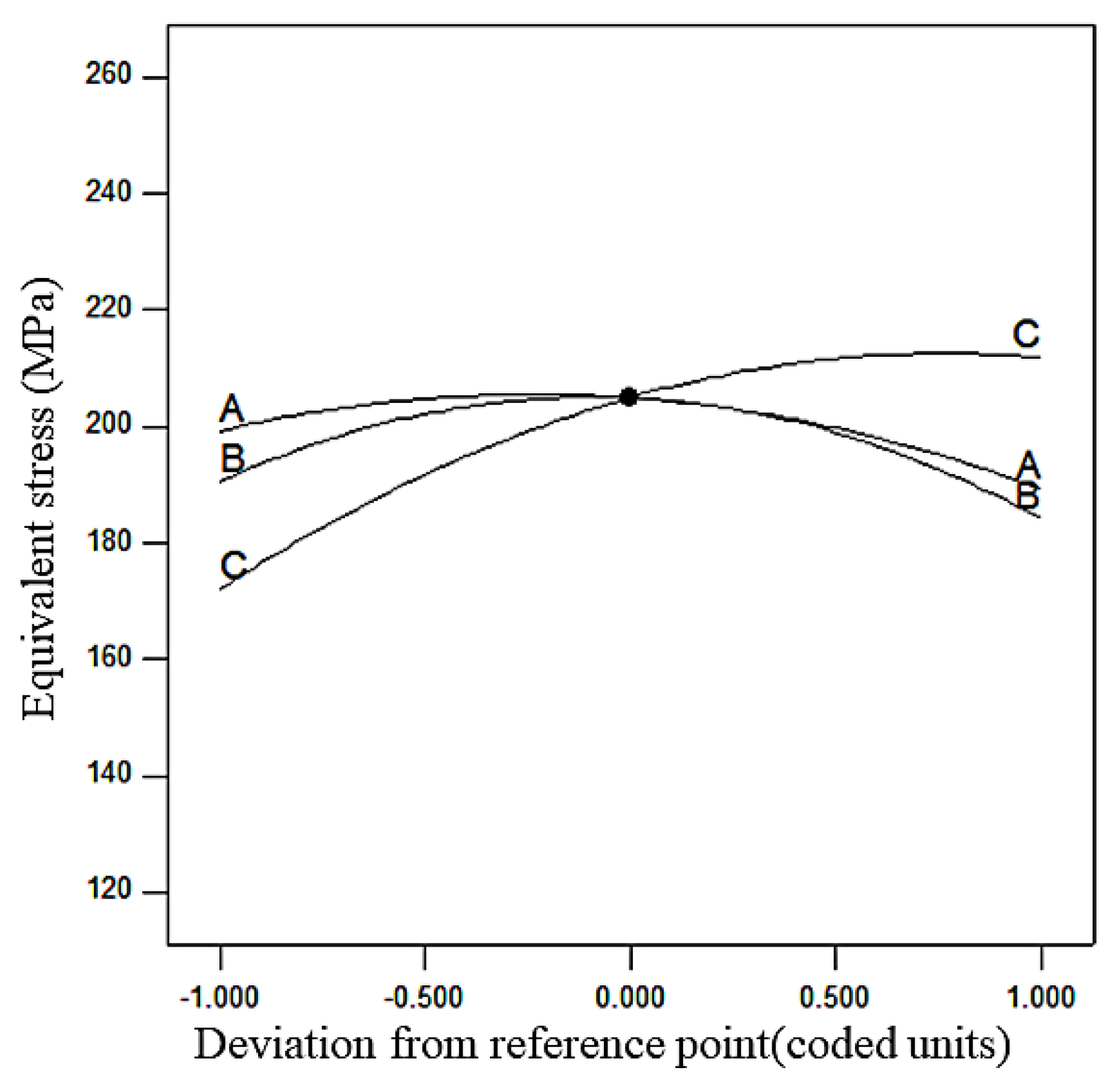
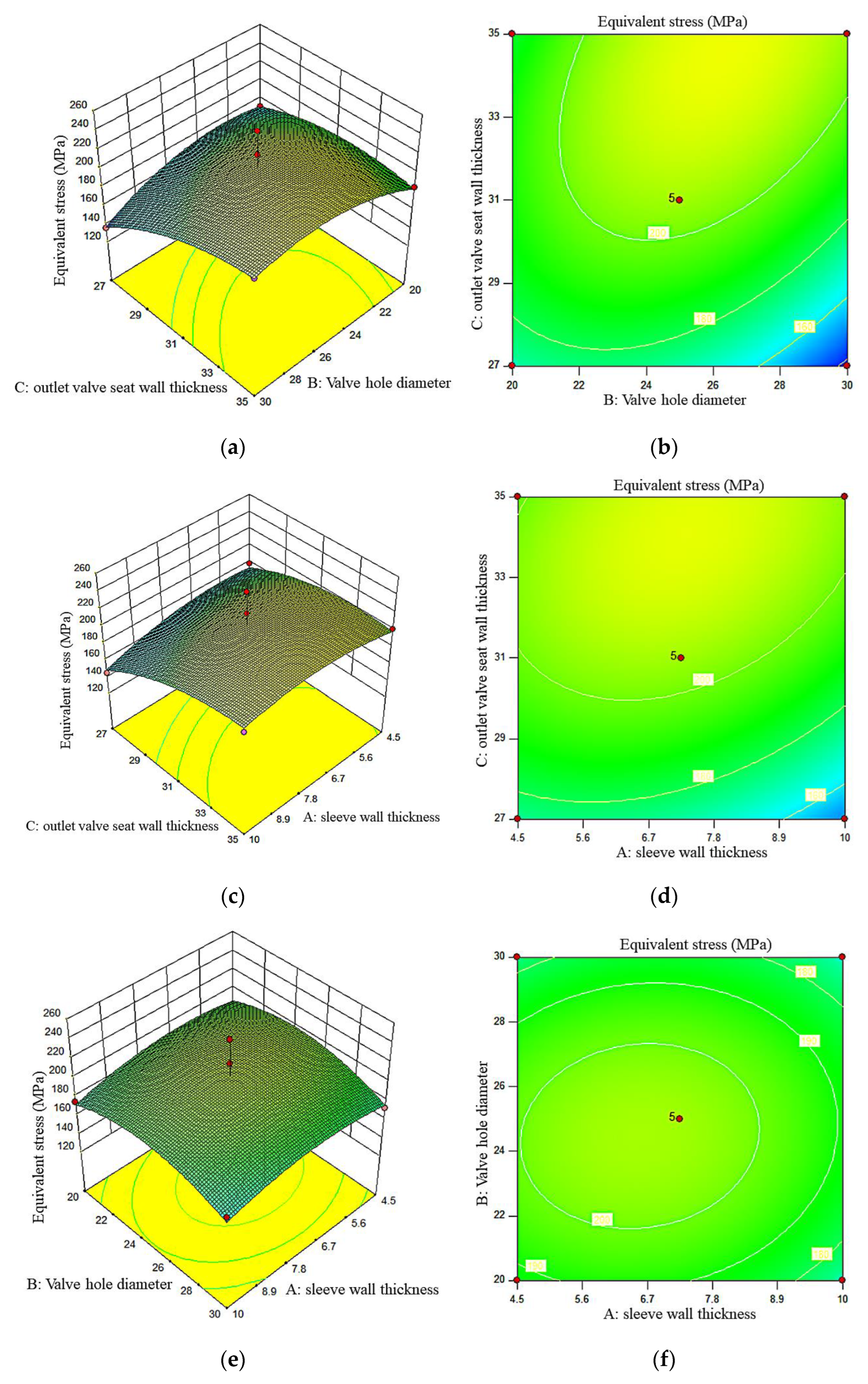
To optimize the structure of the gas regulator at the 20% opening, the sleeve wall thickness, valve bore diameter, and outlet seat wall thickness are confirmed as the parameter variables. The equivalent stress is determined as the objective function, and the response surface method is applied to optimize the structure of the gas regulator. Hence, to obtain the optimal objective function and the optimal solution, that is, when the sleeve wall thickness is 7.25 mm, the valve hole diameter is 25 mm, the outlet seat wall thickness is 31.05 mm, and the gas regulator’s overall displacement and equivalent stress reach the minimum. Lastly, the maximum equivalent stress is 135.62 MPa.

References

1. Ramzan, M.; Maqsood, A. Dynamic modeling and analysis of a high pressure regulator. Math. Probl. Eng. 2016, 2016, 1307181. [Google Scholar] [CrossRef]
2. Hao, X.J.; An, X.R.; Wu, B.; He, S.P. Application of a support vector machine algorithm to the safety precaution technique of medium-low pressure gas regulators. J. Therm. Sci. 2020, 27, 74–77. [Google Scholar] [CrossRef]
3. Zhi, X.Y.; Wang, Y.H.; An, Y. Gas pressure regulator fault diagnosis model based on support vector machine. In Proceedings of the 31th Chinese Control and Decision Conference, Nanchang, China, 3–5 June 2019. [Google Scholar]
4. Changsoo, L.; Heui-Joo, C.; Geon-Young, K. Numerical modelling of coupled thermo-hydro-mechanical behavior of heater experiment–D (HE-D) at Mont Terri rock laboratory in Switzerland. Tunn. Undergr. Space 2020, 30, 242–255. [Google Scholar]
5. Partoaa, A.A.; Abdolzadeh, M.; Rezaeizadeh, M. Effect of fin attachment on thermal stress reduction of exhaust manifold of an off road diesel engine. J. Cent. South Univ. 2017, 24, 546–559. [Google Scholar] [CrossRef]
6. Nariman, N.A. Thermal fluid-structure interaction and coupled thermal-stress analysis in a cable stayed bridge exposed to fire. Front. Struct. Civ. Eng. 2018, 12, 609–628. [Google Scholar] [CrossRef]
7. Mahtab, M.S.; Islam, D.T.; Farooqi, I.H. Optimization of the process variables for landfill leachate treatment using Fenton based advanced oxidation technique. Energy Convers. Manag. 2017, 151, 630–640. [Google Scholar] [CrossRef]
8. Sarikaya, M.; Gullu, A. Taguchi design and response surface methodology based analysis of machining parameters in CNC turning under MQL. J. Clean. Prod. 2014, 65, 604–616. [Google Scholar] [CrossRef]
9. Karimifard, S.; Moghaddaam, M.R.A. Application of response surface methodology in physicochemical removal of dyes from wastewater: A critical review. Sci. Total Environ. 2018, 250, 793–798. [Google Scholar] [CrossRef] [PubMed]
10. Sarafraz, M.M.; Tlili, I.; Tian, Z.; Bakouri, M.; Safaei, M.R. Smart optimization of a thermosyphon heat pipe for an evacuated tube solar collector using response surface methodology (RSM). Phys. Stat. Mech. Its Appl. 2019, 534, 122146. [Google Scholar] [CrossRef]
11. Safariforoshani, M. Thermo-hydro-mechanical analysis of fractures and wellbores in petroleum/geothermal reservoirs. Diss. Abstr. Int. 2013, 75, 324. [Google Scholar]
12. Deissler, R. Turbulent Fluid Motion; CRC Press: Boca Raton, FL, USA, 2020. [Google Scholar]
13. Venkateswarlu, K. Engineering Thermodynamics: Fundamental and Advanced Topics; CRC Press: Boca Raton, FL, USA, 2021. [Google Scholar]
14. Yao, T. Regulator Performance Optimization Study of RTZ-50/0.4FQ Type Gas Regulator; Southwest Petroleum University: Chengdu, China, 2017. (In Chinese) [Google Scholar]
15. ISO 23251; Petroleum, Petrochemical and Natural Gas Industries—Pressure-Relieving and Depressuring Systems. International Organization for Standardization: Geneva, Switzerland, 2019.
Figure 1. FL series gas pressure regulator. (a) Real structure, (b) Simplified structure model.
Applsci 13 06548 g001
Figure 2. FEA model for the gas pressure regulator. (a) Structural model, (b) Fluid model.
Applsci 13 06548 g002
Figure 3. Simulation results for the gas pressure regulator at the 50% opening. (a) Temperature field, (b) Heat flux.
Applsci 13 06548 g003
Figure 4. The temperature and heat flux curves of the valve spool for the gas pressure regulator with different openings.
Applsci 13 06548 g004
Figure 5. Total deformation and stress of the gas pressure regulator at the opening 50%. (a) Total deformation, (b) Equivalent stress.
Applsci 13 06548 g005
Figure 6. Variation of deformation of the gas pressure regulator under different openings.
Applsci 13 06548 g006
Figure 7. Equivalent stress curve of various parts of the gas pressure regulator with different openings.
Applsci 13 06548 g007
Figure 8. Positive probability of residual error.
Applsci 13 06548 g008
Figure 9. Residual Curves. (a) Residual vs. test times, (b) Residual vs. predicted value.
Applsci 13 06548 g009
Figure 10. Perturbation diagram (A: sleeve wall thickness; B: valve hole diameter; C: outlet valve seat wall thickness).
Applsci 13 06548 g010
Figure 11. Response surface and contour map. (a) Relationship among valve hole diameter, outlet valve seat wall thickness, and equivalent stress, (b) Contour map between outlet valve seat wall thickness and valve hole diameter, (c) Relationship among sleeve wall thickness, outlet valve seat wall thickness, and equivalent stress, (d) Contour map between outlet valve seat wall thickness and sleeve wall thickness, (e) Relationship among sleeve wall thickness, valve hole diameter, and equivalent stress, (f) Contour map between valve hole diameter and sleeve wall thickness.
Applsci 13 06548 g011