Estimating Liquefaction Susceptibility Using Machine Learning Algorithms with a Case of Metro Manila, Philippines

Abstract

Soil liquefaction is a phenomenon that can occur when soil loses strength and behaves like a liquid during an earthquake. A site investigation is essential for determining a site’s susceptibility to liquefaction, and these investigations frequently generate project-specific geotechnical reports. However, many of these reports are frequently stored unused after construction projects are completed. This study suggests that when these unused reports are consolidated and integrated, they can provide valuable information for identifying potential challenges, such as liquefaction. The study evaluates the susceptibility of liquefaction by considering several geotechnical factors modeled by machine learning algorithms. The study estimated site-specific characteristics, such as ground elevation, groundwater table elevation, SPT N-value, soil type, and fines content. Using a calibrated model represented by an equation, the investigation determined several soil properties, including the unit weight and peak ground acceleration (PGA). The study estimated PGA using a linear model, which revealed a significant positive correlation (R² = 0.89) between PGA, earthquake magnitude, and distance from the seismic source. On the Marikina West Valley Fault, the study also assessed the liquefaction hazard for an anticipated 7.5 M and delineated a map that was validated by prior studies.

1. Introduction

In geotechnical engineering, soil liquefaction is a critical phenomenon that occurs when saturated or partially saturated soil loses its strength and stiffness, causing it to behave like a liquid during an earthquake or other rapid loading conditions. Therefore, evaluating the resistance of soil to liquefaction is essential for ensuring the safety of infrastructures. [1]. Significant research and studies on liquefaction have been conducted over the past decade, highlighting the significance of understanding this phenomenon [2,3,4,5,6].

When the pore-water pressure in a granular material increases and the effective stress decreases, the material changes from a solid to a liquid state [7]. Typically, this occurs in loose to moderately dense granular soils with inadequate drainage such as sands and gravels. During seismic shaking, the ground undergoes significant movements that cause the rearrangement of soil particles and the collapse of pore spaces, leading to an increase in pore water pressure. This decreases the effective tension between soil particles, weakens the soil’s overall structure, and causes the soil to liquefy and flow. During seismic events, the increase in pore water pressure decreases the effective stress, making the soil even more susceptible to liquefaction [1].

In recent years, there have been numerous instances in which liquefaction events have caused significant structural damage. For instance, the 2011 Christchurch, New Zealand, earthquake was a catastrophic event that caused widespread liquefaction-induced damage to numerous buildings [8]. This included residential, commercial, and public buildings, which suffered varying degrees of structural damage due to liquefaction. Similarly, the Loma Prieta earthquake in 1989 [9], the Tohoku earthquake and tsunami in 2011 [10], and the Niigata-Chuetsu earthquake in 2004 [11] were other notable events where liquefaction caused damage to structures.

In addition, understanding liquefaction enables geotechnical engineers to develop innovative mitigation procedures that reduce the risk of liquefaction-induced damage [12], such as techniques for ground improvement such as soil stabilization [13,14,15]. When sufficient data are available, geotechnical engineers can create susceptibility maps and conduct hazard assessments [16,17] to identify areas with a higher liquefaction risk.

Geotechnical engineering is a complex field that requires a thorough understanding of the soil and geological conditions at a given site. To determine the susceptibility of a site to liquefaction, a comprehensive site investigation is a crucial first step. This investigation requires the drilling of boreholes, such as the Standard Penetration Test (SPT) [18], and the collection of soil samples for laboratory analysis to determine the physical and engineering properties of the soil. These properties include grain size distribution, moisture content, density, shear strength, and consolidation characteristics, among others, which are critical in assessing the site’s liquefaction susceptibility.

Typically, the results of the site investigation are documented in geotechnical reports that are unique to each project and contain vital information on the soil and other relevant factors. However, it has been observed that after the completion of a construction project, many of these reports are frequently stored unused. These unused reports have the potential to provide valuable information when collected, consolidated, and integrated to identify potential challenges, such as liquefaction, which may not be evident in a single report [19].

The development of fundamental soil testing techniques, such as visual inspection and manual testing, in the eighteenth century paved the way for significant advancements in geotechnical engineering. The construction of foundations in challenging soils, such as soft clay, sand, and rock, was one such area of advancement [20]. In addition, correlations between soil grain size distribution and engineering behavior have been established, marking an important development in the field of geotechnical engineering. In situ and laboratory testing continue to be the preferred methods for determining construction project design parameters. In the early stages of a project, when site investigation data may not yet be available, correlations based on historical laboratory or field data are useful [21,22] for estimating the subsurface condition of a site.

When determining liquefaction susceptibility, the cyclic resistance ratio (CRR) and cyclic stress ratio (CSR) are vital parameters. The CRR reflects the soil’s resistance to liquefaction, as determined by laboratory analysis of soil samples. CSR is dependent on seismic loading conditions and soil characteristics at a particular site [20,23,24,25,26,27]. However, developing correlations has been difficult due to the scarcity of dependable and exhaustive data sets. To address this challenge, researchers have integrated empirical data and developed calibrated models to improve the accuracy of predictions and increase knowledge of soil behavior. These advancements in soil testing and correlations have substantially advanced the field of geotechnical engineering.

Geotechnical engineering has seen significant advancements in modeling techniques—from simple analytical methods to complex numerical modeling techniques. Initially, mathematical equations were used to predict soil behavior, but recent research has shown that machine learning is a reliable method for predicting geotechnical parameters, [28,29,30], particularly liquefaction [31,32,33].

Numerous investigations have employed machine learning algorithms to forecast geotechnical characteristics, such as the potency of stabilized soils [28]. Some of these investigations have employed several models concurrently to assess their efficacy [34].

Empirical evidence suggests that the precision of these models is significantly influenced by the volume of data utilized, as a larger dataset leads to more precise predictions [35].

Geostatistics, a field of study that encompasses techniques such as kriging and inverse weighted triangle, has conventionally been employed to interpolate geotechnical characteristics and generate digital maps [36]. However, geostatistics has limitations when it comes to estimating the distribution of numerical data, which has led to alternative techniques such as machine learning being explored. The integration of machine learning and geostatistics has the potential to facilitate the estimation of geotechnical properties in regions with limited data availability. Moreover, this approach can be effectively employed to estimate geotechnical properties that exhibit high anisotropy [36,37].

The emergence of digital technology has significantly transformed data collection in the field of geotechnical engineering. Geotechnical engineers are now able to employ geospatial intelligence as a promising tool to analyze and visualize geographic information of sites that are susceptible to liquefaction, thanks to the advent of various tools. This technology allows the processing of geotechnical data and reports without physically visiting the location, making it more efficient and effective in planning projects [38].

In geospatial intelligence, surficial studies were commonly conducted since data were easily obtainable, examples are deformations of cultural heritage structures [39], maritime safety [40], flood risk [41], urban land use [42], land subsidence [43], rainfall-runoff relationship [44], and forest fire spread [45]. The utilization of geospatial intelligence in the analysis of liquefaction phenomena has received comparatively little attention, with only a limited number of investigations having been conducted to date.

The present study endeavors to fill the gap by utilizing machine learning algorithms to estimate the vulnerability of liquefaction in a case study conducted in Metro Manila, Philippines. The study will examine multiple geotechnical factors that have been modeled by algorithms to evaluate the probability of liquefaction taking place in the designated research region. This research aims to utilize geospatial intelligence and machine learning algorithms to offer significant insights into the incidence of liquefaction.

2. Methodology

This research outlines a thorough approach to evaluating the vulnerability of soil liquefaction in a seismic zone with a high level of risk. The methodology comprises a series of sequential steps encompassing data collection, data processing, microzonation, borehole density determination, machine learning training and modeling, and validation. The research centers on the metropolitan region of Manila, which is characterized by a high population density and urbanization, rendering it an especially susceptible site for liquefaction.

2.1. Data

In order to facilitate the programming code and machine learning modeling, important geotechnical investigation data were extracted from the borehole log and systematically arranged in a spreadsheet format. The parameters that have been extracted comprise of the project information, geographical location, coordinates, ground altitude, subterranean water level, Standard Penetration Test (SPT) N-values, Unified Soil Classification System (USCS) soil type, proportion of fines, grain size distribution data, as well as Atterberg limits, namely, liquid limit (LL) and plastic limit (PL). Furthermore, empirical data obtained from previously published research studies were methodically digitized and collected via a comprehensive literature search process. The methodology employed entailed the systematic exploration and synthesis of information from established literature sources, with the aim of attaining a thorough comprehension of pre-existing data and enhancing the ability to establish meaningful associations, ultimately leading to improved information accessibility.

The process of calibrating data from various sources is an essential component in attaining a comprehensive understanding of the available data. This process enables better correlations and enhances accessibility to information. In order to support the research, seismic data were incorporated, encompassing significant earthquake occurrences (including magnitude and epicenter location), the latitude and longitude of PGA stations where these events were recorded, and the latitude and longitude of active faults in the surrounding area, including the head and tail of said faults. These data hold significant importance in assessing the vulnerability of a region to the phenomenon of soil liquefaction.

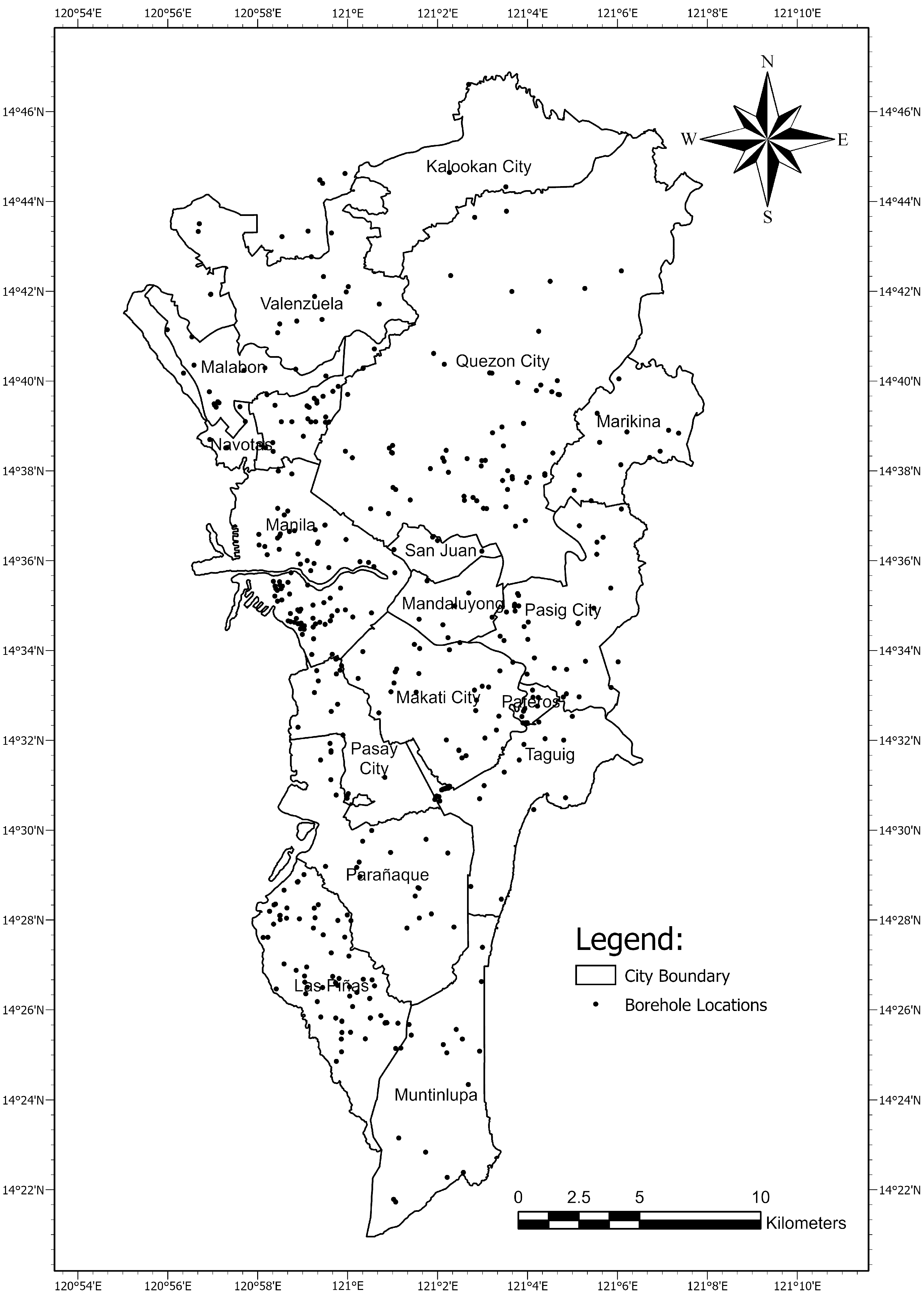
2.2. Density of Boreholes

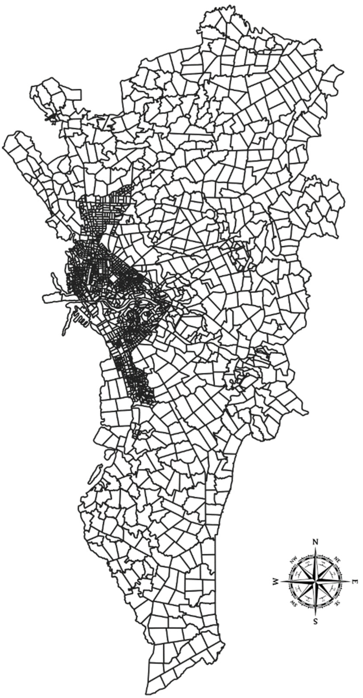
In terms of the density of boreholes per city, 1 borehole/km² was followed to ensure that a borehole can represent a square kilometer of a city. The density of boreholes per city was checked using Equation (1):

$$\mathrm{D}=\frac{B}{A}$$

(1)

where D is the density of boreholes (boreholes/km²), B is the number of usable boreholes, and A is the area covered (km²).

2.3. Microzonation

In this study, microzonation, which involves reducing a large area into smaller areas, was accomplished using Geographic Information System (GIS) software. The area of each zone was calculated, and any large zones with an area greater than 1 km² were further subdivided into smaller zones. Once the areas of the zones met the requirements of this study, their centroids were located using a latitude and longitude format.

2.4. Training and Modelling

2.4.1. Modelling Process

Machine learning is a powerful tool that automates the creation of models and is categorized under artificial intelligence. Using the concept that algorithms can learn from data, recognize patterns, and make decisions with minimal human intervention, machine learning has become necessary for analyzing larger and more complex datasets, producing accurate results at a faster rate, even when dealing with massive amounts of data [46].

There are two primary types of models in supervised learning, a subcategory of machine learning: regression and classification. Classification models accurately assign test data to specific categories or classifications and are suited for non-numerical data types such as texts, boolean values, and dates. Regression models identify the relationship between dependent and independent variables in numerical data.

Machine learning algorithms make predictions based on data by constructing mathematical models from multiple datasets, including training, validation, and test sets. The three-step process of utilizing training, validation, and test data sets is essential for developing accurate and reliable machine learning models. The training data set is used during the learning process and for fitting the model parameters. The validation data set is used to evaluate the model and provide an unbiased assessment of its fit to the training data, while also tuning the hyperparameters of the model [47].

Commonly used parameters for evaluating the performance of trained models include accuracy rates, coefficient of determination (R²), and root mean square error (RMSE). Depending on the type of model, these evaluation parameters or correlation structures are utilized differently. For classification models, accuracy rates are commonly used as a performance metric, whereas for regression models, the coefficient of determination and root mean square error are frequently used.

In the process of training and modeling, collected data are used to train multiple regression and classification machine learning models. After that, their performance parameters are compared to determine which model is superior. To further optimize the performance of the winning model, hyperparameters are modified through an iterative process of tuning hyperparameters to achieve the best results possible. Overall, machine learning is an indispensable instrument for automating data processing and developing reliable and precise models.

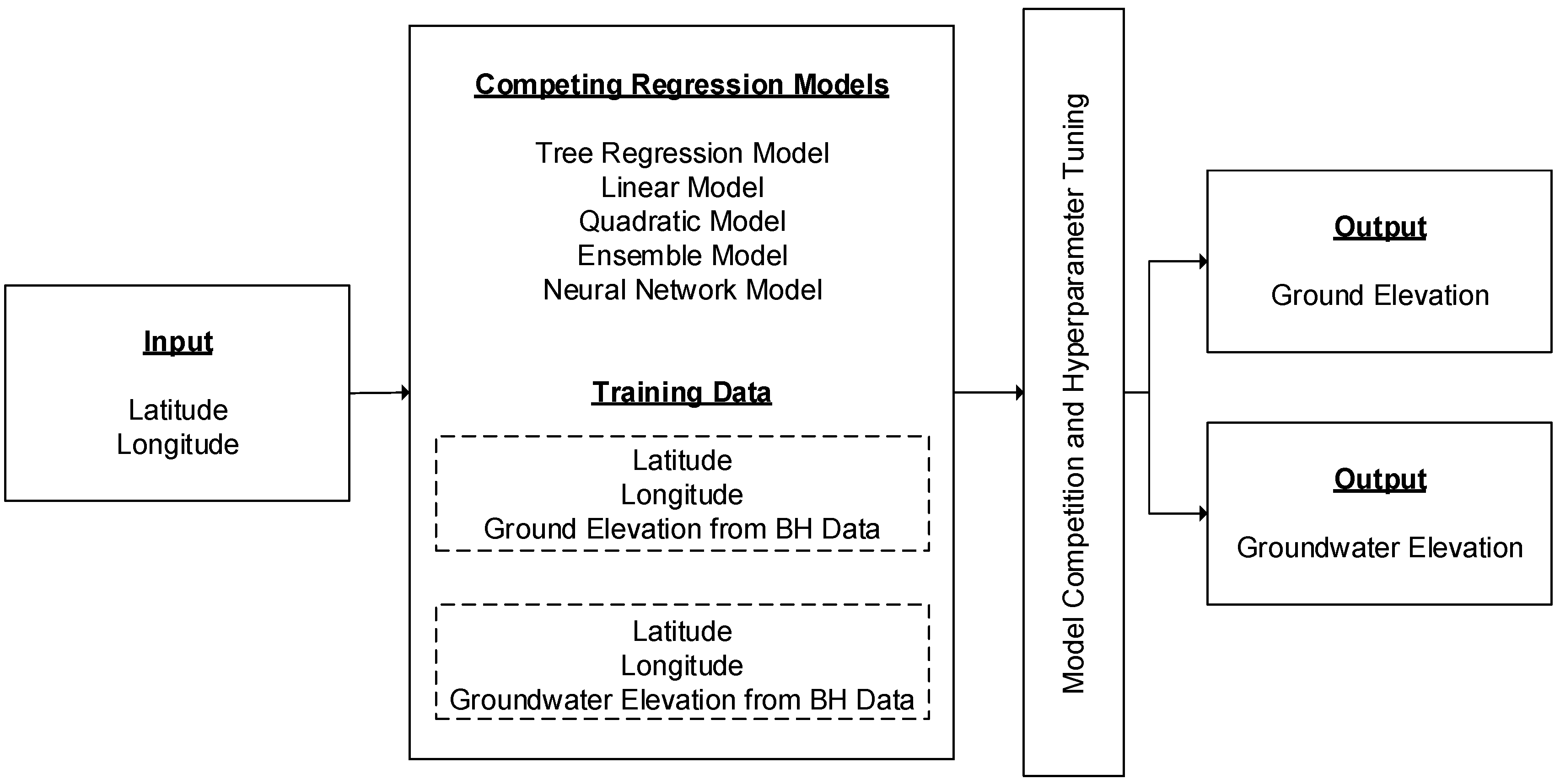
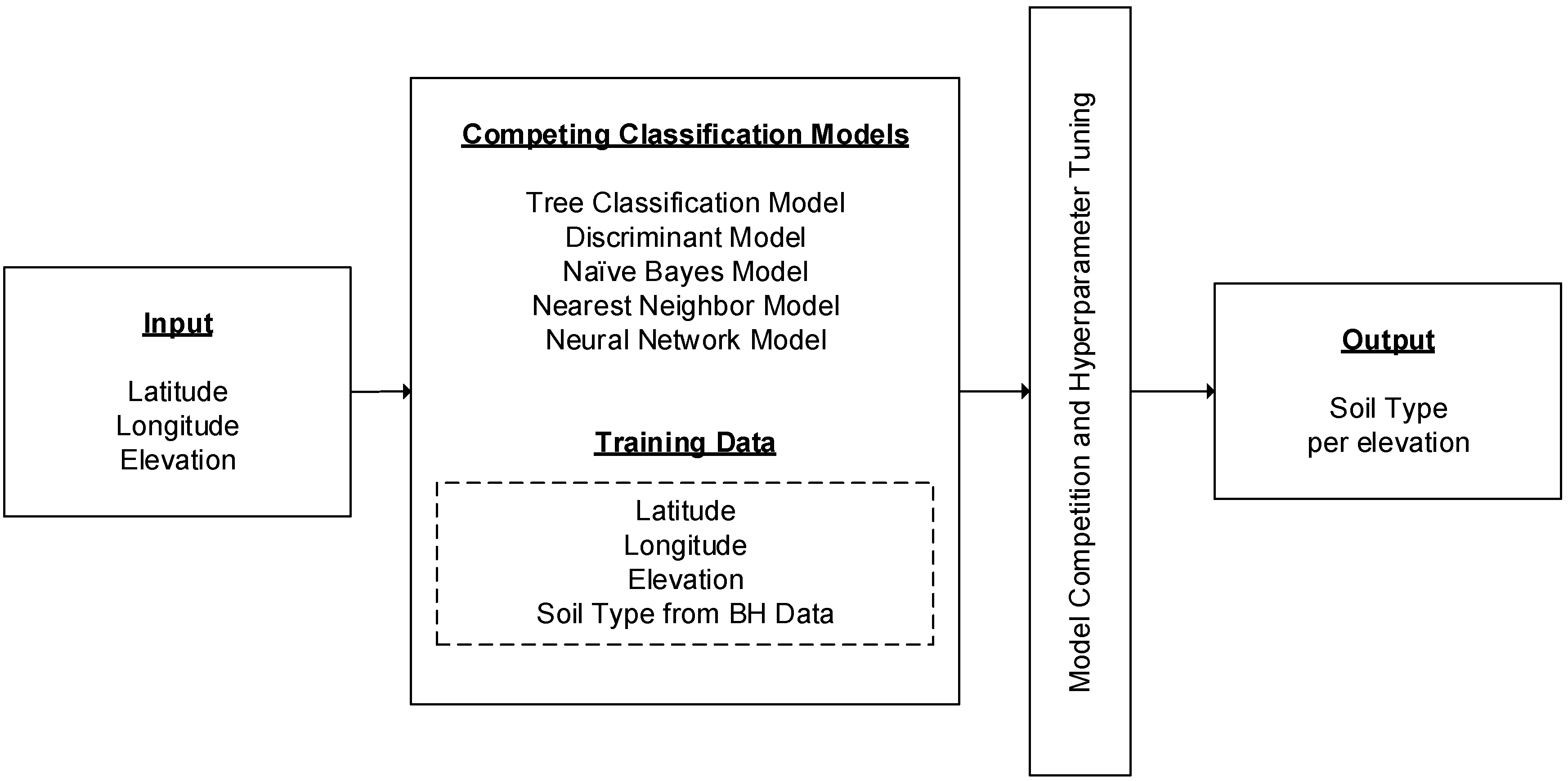
2.4.2. Modelling of Site-Specific Properties

Using site-specific properties such as ground elevation and groundwater elevation, the process of estimating initial parameters for locations without data consisted of using site-specific properties such as ground elevation and groundwater elevation. As depicted in Figure 1, the latitude and longitude of each location were used as input variables to train models using the geotechnical investigation report’s source data. Then, hyperparameter tuning was performed to enhance the winning model. Once the ground elevation was determined, it was extended to a depth of 20 m below mean sea level, allowing for accurate estimation of ground properties in regions where data was initially lacking. Using a combination of data-driven modeling and geospatial analysis, this method produced accurate estimates for these crucial site-specific properties.

As depicted in Figure 2, the procedure for estimating soil type for each layer in an area with no available data was similar to that used for determining ground and groundwater elevation. In this instance, however, classification models were employed rather than regression models, as non-numerical variables are typically assigned to soil types. Figure 3 depicts the estimation of additional site-specific geotechnical properties, such as SPT N-values, fines content, liquid limit, and plastic limit, using regression models. Notably, when an SPT N-value of 50 was encountered during the estimation process, the corresponding layer was classified as rock. The only distinction between this procedure and the modeling of ground and groundwater elevation is the inclusion of layer elevation in the input and training data.

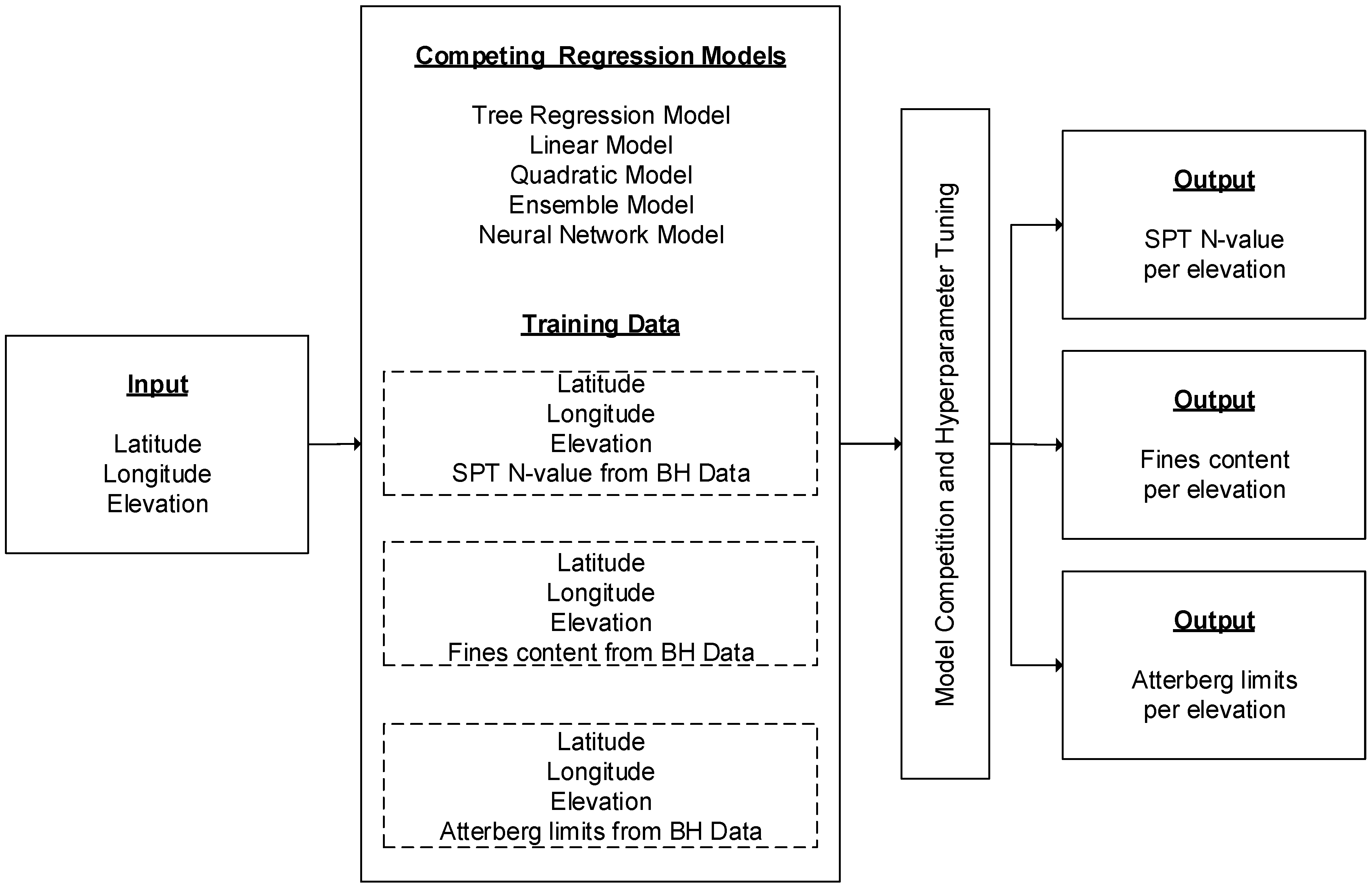
2.4.3. Modelling of Geotechnical Strength Parameters

Terzaghi’s revolutionary contribution to geotechnical engineering was the development of a theory that could be used to determine the ultimate bearing capacity of shallow foundations. This theory takes into account important factors such as the weight of the soil and the cohesive forces acting on the foundation, making it an indispensable tool for engineers and scientists.

The estimation of the soil’s unit weight, which is based on various geotechnical parameters such as angle of internal friction and cohesion, is a crucial factor in determining the soil’s strength. Collecting data from previous studies that describe the soil’s properties, location, and SPT N-value is necessary for estimating the unit weight of soil. It is important to note that unit weight values can vary depending on soil particle composition, saturation level, and other environmental variables.

Table 1. Determination of soil group for unit weight.

Soil Group	Soil Type
Coarse-Grained Soils	GW, GP, GM, GC, SW, SP, SM, SC
Fine-Grained Soils	ML, CL, OL, MH, CH, OH

was used by researchers to classify soil into the appropriate groups. This table helped them classify the soil according to its properties, allowing for more accurate and reliable data collection. In addition, Figure 4 illustrates the method for determining the unit weight of a soil layer. This procedure utilizes four different unit weight values based on the layer’s location (above or below the groundwater table) and its soil type.

These parameters include moist unit weight of coarse-grained soil (kN/m³), saturated unit weight of coarse-grained soil (kN/m³), moist unit weight of fine-grained soil (kN/m³), and saturated unit weight of fine-grained soil (kN/m³).

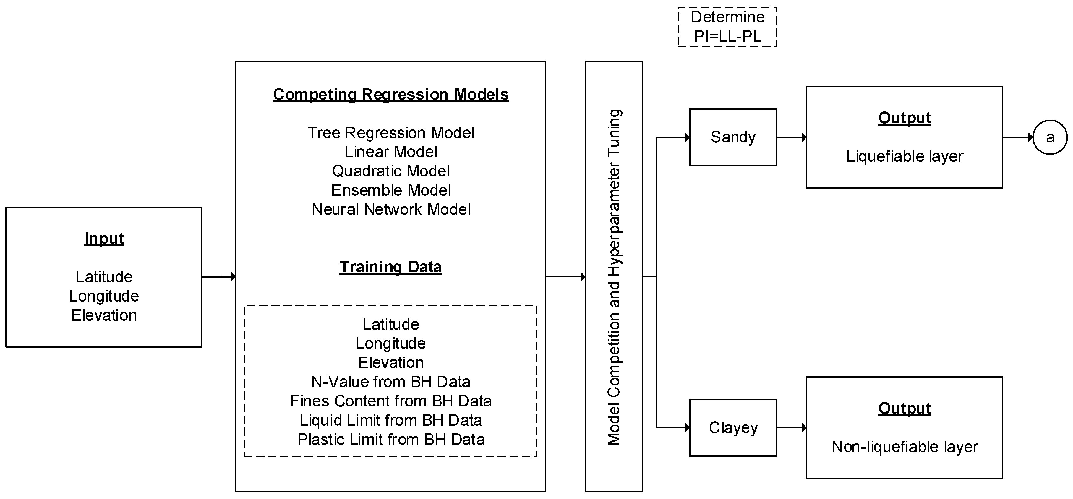
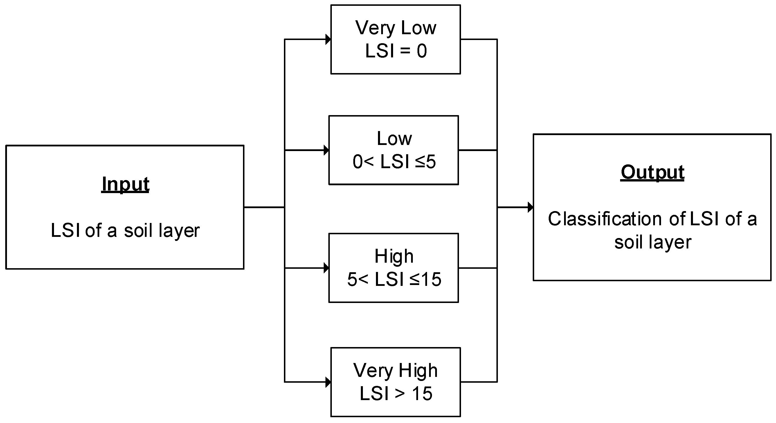
2.4.4. Modelling Liquefaction Susceptibility

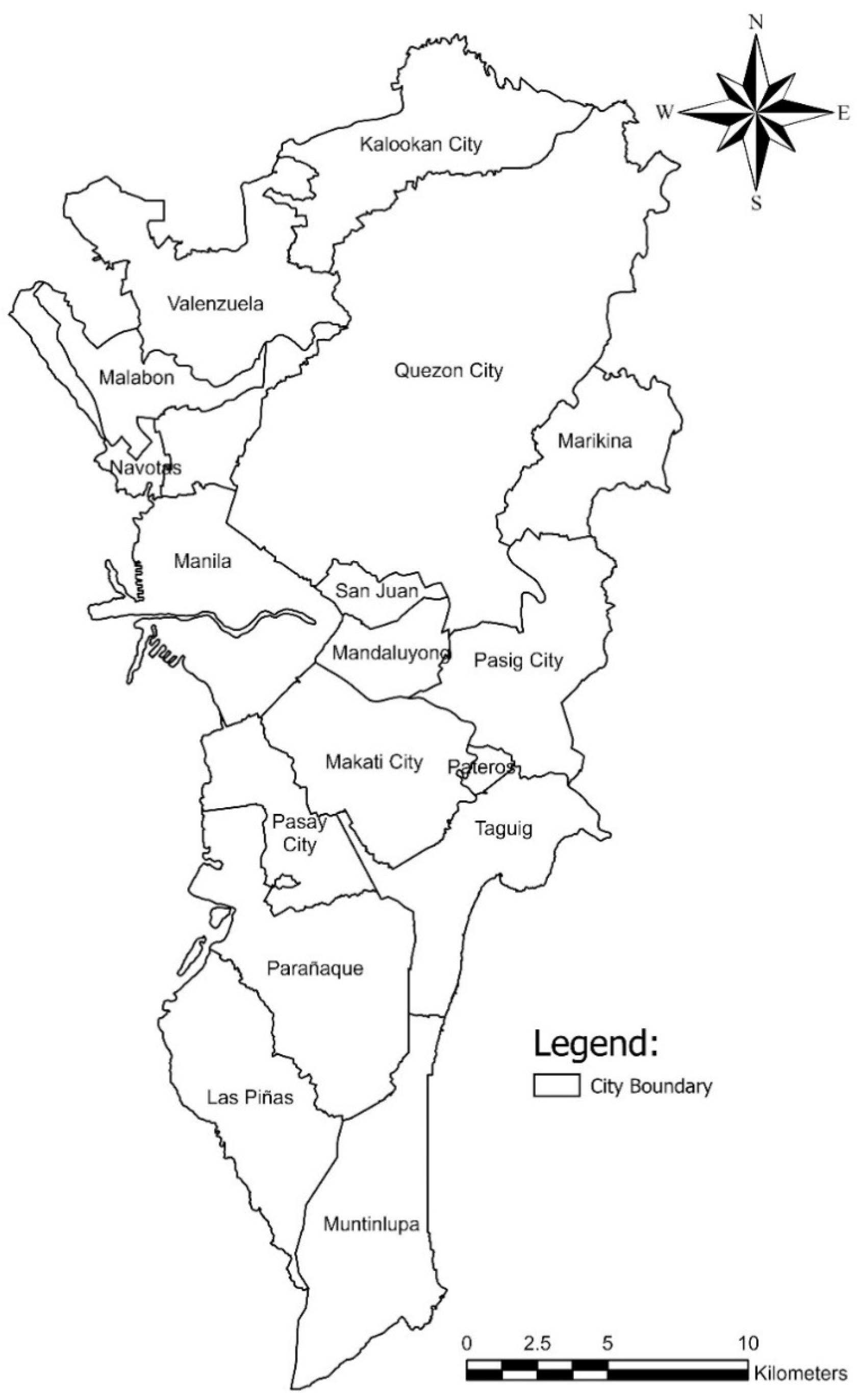
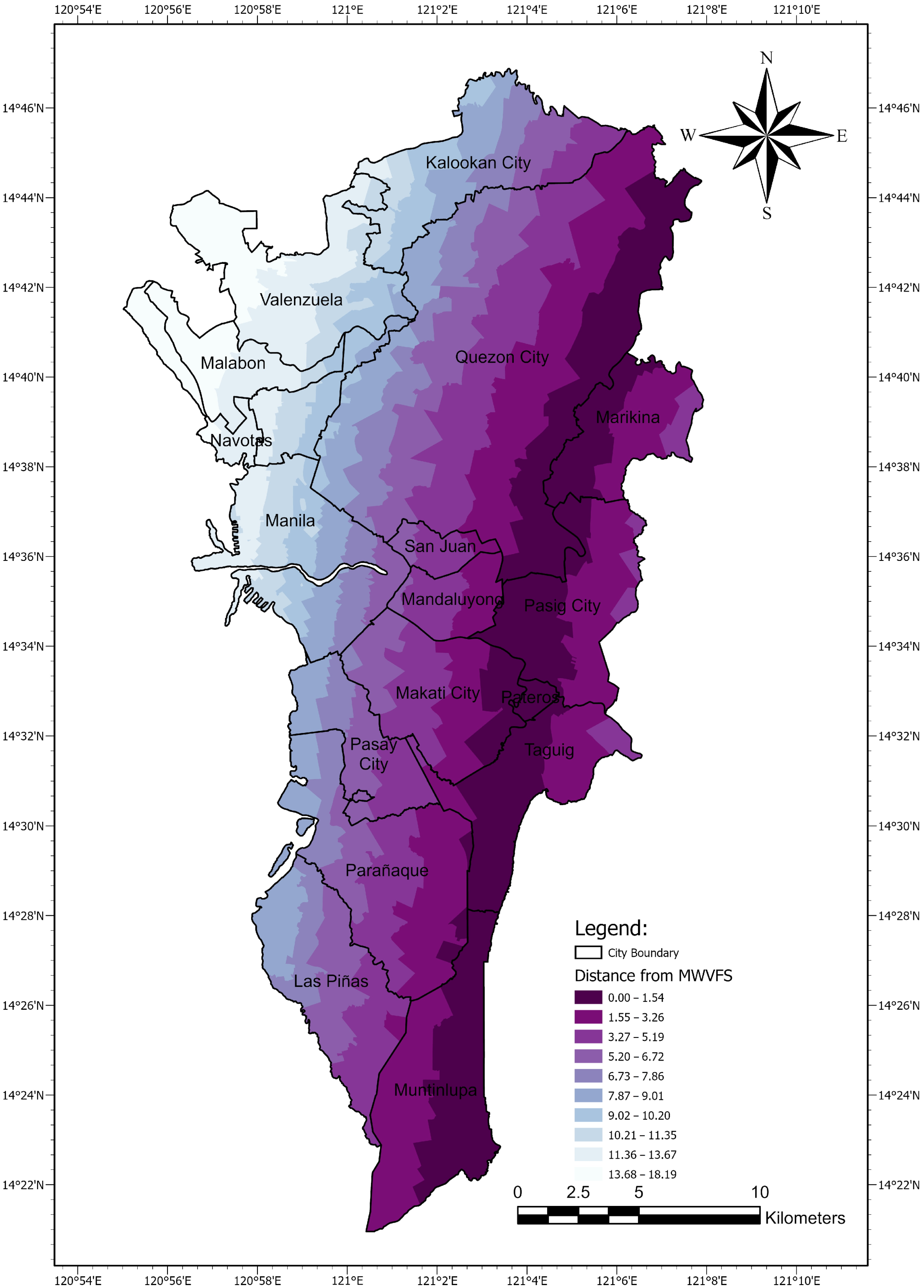
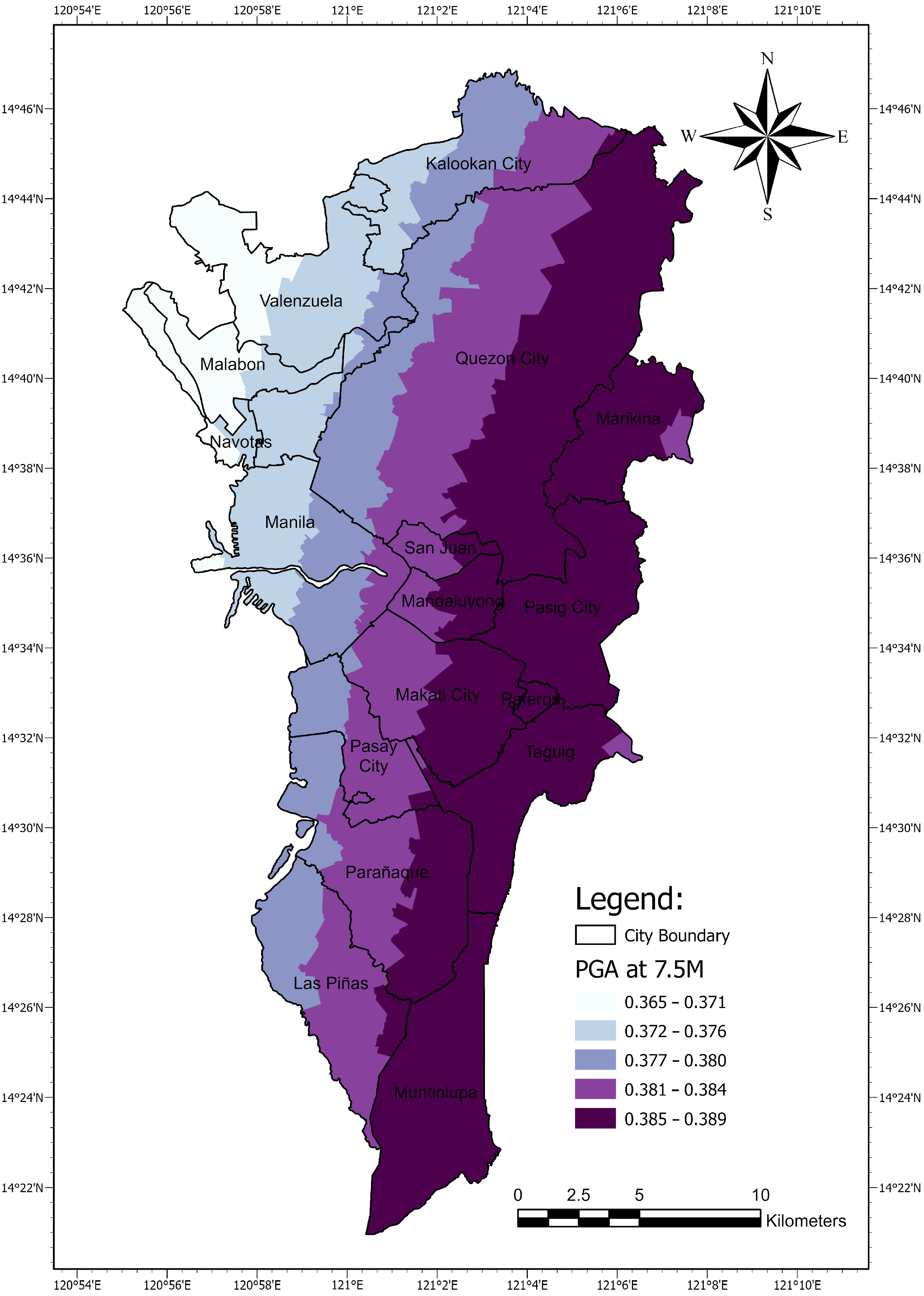
In geotechnical engineering, particularly in earthquake-prone regions, the liquefaction susceptibility of soil is a crucial factor to consider. Idriss et al. (2004) [1] developed a multi-step method for determining the susceptibility of soil to liquefaction.

First, the method classifies the soil as either clayey or sandy based on its Atterberg limits. Atterberg limits are the moisture contents at which a soil changes state from solid to liquid (liquid limit) and from liquid to semisolid (plastic limit). As shown in Figure 5, sandy soil is initially classified as liquefiable while clayey soil is classified as non-liquefiable.

Once classified as liquefiable, the initial input was the number of blows or penetration resistance (SPT N-value) registered for each penetration interval at a given depth. Due to the variety of hammer designs used in field research, corrections were made using hammers with an efficiency of approximately 60%, and an equation for the correction of SPT N-values was used. Once the corrected SPT N-value was determined, the equivalent clean sand value $({(N_1)}_{60cs})$ and cyclic resistance ratio (${CRR}_{7.5}$) were computed. However, the ${CRR}_{7.5}$ equation is only valid for ${(N_1)}_{60cs}<30$. Since there are clean granular soils that are too dense to liquefy, ${(N_1)}_{60cs}\ge 30$, it is further classed as non-liquefiable.

After determining CRR, the seismic demand on a soil layer is further computed in terms of the cyclic stress ratio (CSR). The initial process is to analyze the Stress Reduction Coefficient ($r_d$) based on the depth of each soil layer, z, initially estimated. At a depth of more than 23 m below ground elevation, Youd et al. noted that no occurrences of soil liquefaction were observed, thus, these depths were considered non-liquefiable.

Aside from r_d, the peak ground acceleration (PGA) is also an essential parameter for CSR. PGA is the maximum surface ground acceleration that occurred during an earthquake shaking at a particular location, a deterministic seismic hazard assessment (DSHA) approach was used to estimate PGA, wherein it is based on the expected earthquake magnitude for a specific seismic source and the minimum distance from the site to the fault source. Another essential parameter in determining CSR is the total and effective overburden stresses, the computation is based on the unit weight of the soil being analyzed and groundwater table elevation. Lastly, the factor of safety (FS) against soil liquefaction is computed in terms of CRR, CSR, and magnitude scaling factor (MSF).

Once the factor of safety for each layer is determined, the calculated probability of liquefaction (PL) is shown in Equation (2). Consequently, the formula depicted in Equation (3) was used to determine the liquefaction severity index (LSI), which is used to evaluate the liquefaction hazard until 20 m below ground elevation. Thereafter, classifications of LSI from very low risk to very high risk were employed, as shown in Figure 6.

$$P_L=\frac{1}{1+{\left(\frac{FS}{0.96}\right)}^{4.5}}$$

(2)

where the probability of liquefaction (P_L) is computed using the calculated factor of safety (FS).

$$LSI={\int }_0^{20}{P}_L\left(z\right)\left(10-0.5\right)dz$$

(3)

where the liquefaction severity index (LSI) is computed using the probability of liquefaction (P_L) and the depth of the soil layer (z, in m).

2.5. Case Study

Metro Manila, also known as the National Capital Region (NCR), was the location of the study. This region encompasses 619.57 square kilometers and consists of the sixteen cities and one municipality depicted in Figure 7. In the region, there are a total of 1690 Barangays. To collect the necessary data, two primary sources were consulted. First, reports on geotechnical investigations were gathered from both private companies and local government agencies. Second, seismic data were obtained from PHIVOLCS, which provided information on significant earthquake events, including their magnitude and epicenter location. In addition, the location of PGA stations where these events were recorded and the location of active faults in the region, including their head and tail latitude and longitude, were also recorded.

2.6. Validation

Importantly, assessing the ability of a model requires evaluating its level of accuracy. To accomplish this, the model must be evaluated using data that was not utilized during training. We can determine the model’s performance by testing its ability to generalize and make accurate predictions on new data. The accuracy rate is a commonly employed metric for evaluating the performance of a model. It quantifies the proportion of accurate predictions made by the model using the test data. A higher accuracy rate indicates that the model can predict future outcomes with greater precision, making it more reliable and applicable to real-world situations. In conclusion, evaluating a model’s accuracy using previously unused data is essential for determining its ability to make accurate predictions, and the accuracy rate is a crucial performance metric.

3. Results and Discussions

3.1. Models

3.1.1. Site-Specific Models

In this study, site-specific characteristics were utilized as model inputs. For example, the SPT N-values and groundwater elevation were used to calculate the unit weights of a soil layer. In cases where data were unavailable for specific locations, the study collected site-specific geotechnical data, including fines content, soil type, and ground elevation, to train and develop machine learning models.

Regression models are utilized for numerical data, whereas classification models are utilized for non-numerical data. Various performance parameters are compared during model training to determine the optimal deployment model. In this study, it was determined that the Tree regression model provided the best fit for the available data, shown on

Table 2. Coefficient of determination (R²) of the site-specific models.

Parameter	Tree	Linear	Quadratic	Ensemble	Neural Network
Ground Elevation	0.99	0.44	0.71	0.98	0.93
Groundwater Table Elevation	0.99	0.44	0.70	0.97	0.92
SPT N-value	0.88	0.09	0.25	0.50	0.46
Fines Content	0.76	0.05	0.16	0.48	0.30

and

Table 3. Root mean square error (RMSE) of the site-specific regression models.

Parameter	Tree	Linear	Quadratic	Ensemble	Neural Network
Ground Elevation	0.00	2.81	2.50	1.24	1.80
Groundwater Table Elevation	0.00	2.95	2.62	1.30	1.89
SPT N-value	7.33	20.24	18.41	15.09	15.73
Fines Content	13.78	27.60	25.97	20.38	23.75

. The algorithm employed by the tree model repeatedly divides the data into partitions based on latitude, longitude, and elevation, as well as the output variable.

With R² values ranging from 0.76 to 0.99, the trained models for ground elevation, groundwater table elevation, SPT N-value, and fines content demonstrated a very strong positive relationship. The lowest RMSE values were also observed for the tree model, indicating a good fit with the data. In addition, with an RMSE of 0.00 m for both the ground elevation and the groundwater table elevation, the tree model provided a perfect fit.

Utilizing the tree model in geotechnical site-specific models has numerous benefits. It requires less work during data preparation and preprocessing, and data normalization and scaling are unnecessary. In addition, missing values in the data do not have a significant impact on the process of constructing a tree, which is especially advantageous in instances where geotechnical investigation reports may contain insufficient data.

In previous sections, the number of usable borehole data was determined by examining the R² and RMSE values. A comparison was conducted to determine how the number of collected data impacts the performance of machine learning models that have been trained. As anticipated, the results demonstrated that as the density of the boreholes increased, the RMSE decreased and the R² increased, resulting in improved model performance. It is commonly understood that insufficient training data can result in less accurate estimates. Similarly, insufficient testing data can lead to overly optimistic results and a high degree of variation.

The winning model’s performance parameters, R² and RMSE, were enhanced through hyperparameter tuning. Since the winning model is the tree model, the number of leaves was the hyperparameter being tuned. The performance of the tree regression model declined as the number of leaves increased, thus, “2” leaves were utilized. This is because a small change in the model can result in a substantial change in the tree’s structure, leading to greater variability.

For non-numerical data such as soil type, classification machine learning models were used to determine the soil types of locations for which no data were available. For classification machine learning models, accuracy rates were used as performance indicators as compared to regression models.

The nearest neighbor model had the highest rate of accuracy among competing models for predicting soil types based on proximity to an unknown layer, shown in

Table 4. Accuracy rates of the site-specific classification models.

Parameter	Tree	Discriminant	Naive Bayes	Nearest Neighbor	Neural Network
Soil Type	70.2	42.8	53.2	93.9	56.3

. Typically, the estimate is based on a majority vote, which means that the soil type that is most frequently represented around the unknown data point is the estimate.

Site-specific models have significant limitations despite their accuracy in predicting ground elevation, groundwater table elevation, SPT N-value, fines content, and soil type. Due to the large number of variables involved, including spatial relationships, there is no particular equation that can represent them. Therefore, there is no benefit to converting the internal models into equations. These trained site-specific models are therefore commonly referred to as black boxes.

3.1.2. Calibrated Models

The collected data from geotechnical investigations can be repurposed to generate calibrated models that estimate the spatial geotechnical properties of other sites for which no data are present. Once calibrated models have been developed, they can be deployed across multiple locations in a region, enabling the delineation of maps. Calibrated models were developed and characterized as soil strength, soil behavior, and liquefaction susceptibility were developed. In contrast to site-specific models, which lack an equation form, calibrated models are trained to include fewer parameters to represent the relationship between parameters via an equation. Site-specific models have the disadvantage of being less interpretable than calibrated models. By using an equation to represent the relationship between parameters, it is easier to comprehend how the input parameter changes affect the output. This makes calibrated models a valuable tool for comprehending soil behavior and strength and predicting the probability of liquefaction.

In soil mechanics, the unit weight of the soil is an essential parameter that plays a significant role in numerous geotechnical engineering analyses. The unit weight is affected by several variables, including the soil’s water content and the level of compaction. To obtain precise results, it is necessary to calibrate the unit weight parameter based on its location and soil group. To accomplish this, four distinct calibrated models for the unit weight of the soil were developed based on its location and soil group. These models include the wet unit weight of coarse-grained soil, the dry unit weight of coarse-grained soil, the wet unit weight of fine-grained soil, and the dry unit weight of fine-grained soil.

The natural in-situ unit weight of soil located above the groundwater table is the moist unit weight. The data on moist unit weight were mined and calibrated to enable data manipulation and facilitate the transformation of raw data into novel insights. As a result, machine learning techniques were used to develop and train the unit weight models. The neural network regression model has the strongest positive relationship (R² = 0.70) among the competing algorithms. Between SPT N-values 0 and 15, a sudden increase in unit weight can be observed, indicating a range from very loose to loose. In addition, beginning with N-values between 15 and 50, the unit weight increases slowly but steadily, as demonstrated by Equations (4) and (5).

$${\gamma }_{moistCG}=0.2868\mathrm{N}+12.559$$

(4)

$${\gamma }_{moistCG}=0.1066\mathrm{N}+15.171$$

(5)

where ${\gamma }_{moistCG}$ is the moist unit weight of coarse-grained soils (kN/m³), N is the SPT N-value, and the SPT N-value range: 1 ≤ N ≤ 15 for Equation (4), and 15 < N ≤ 50 for Equation (5). A new trend in unit weight estimation has emerged that differs from previous trends established by notable researchers [23,47,48,49,50,51]. These earlier studies examined the relationship between SPT N-values and the moist unit weight and discovered a consistent increase. However, a significant limitation of these earlier models was that they did not account for the situation in which an SPT value of “0” was present. For instance, both Puri’s (2018) and Rahman’s (2019) models include an intercept when the SPT N-value is “0,” leading to unreliable estimates of 12.25 kN/m³ and 16 kN/m³, respectively. Therefore, this new trend in unit weight estimation is significant due to its capacity to address and rectify the flaws of previous models.

The quadratic model won in the competition between models for the moist unit weight of fine-grained soils, as represented by Equation (6). The sparse nature of the collected data hinders the effectiveness of the model, resulting in a weak relationship with an R² value of 0.16. Consequently, the linear model is also a viable option, although its performance is inferior to that of the quadratic model.

$${\gamma }_{moistFG}=0.0008{\mathrm{N}}^2+0.0418\mathrm{N}+14.849$$

(6)

where ${\gamma }_{moistFG}$ is the moist unit weight of fine-grained soils (kN/m³), and N is SPT N-value, with a range of 1< N ≤ 50.

The proposed model follows the trend established by previous researchers [20,48], which establishes a direct correlation between the SPT N-Value and the soil unit weight. Peck et al. [20] explain that this trend is attributable to the compaction of soil particles and the presence of an adequate amount of water in the soil layer above the groundwater table. As the N-Value increases, so does the relative density of the soil particles, resulting in greater compaction and, ultimately, a rise in unit weight.

In addition, the saturated unit weight is a distinct parameter used for subsurface soil layers. Above the groundwater table, soil particles are not saturated with water, resulting in a higher unit weight. However, the trained models contradict this notion because most saturated soil layers are located below the groundwater table and are denser, accounting for the additional weight of water due to its saturation in this property. Therefore, these soil layers tend to have a higher unit weight, with a minimum of 15.63 kN/m³ and a maximum of 21.53 kN/m³ for the saturated unit weight. The linear model is the preferred and most accurate model for estimating the saturated unit weight of both coarse-grained and fine-grained soil layers. With an R² value of 0.30, the linear model for coarse-grained soil has a moderately positive relationship. The linear model for fine-grained soil, on the other hand, has a strong positive relationship, with an R2 value of 0.61. The coarse-grained soil model has a lower R² value than the fine-grained soil model, indicating that there is less sparsity in the data. The model for the saturated unit weight of coarse-grained soils is represented by Equation (7), while the model for the saturated unit weight of fine-grained soils is represented by Equation (8). Based on the trend described by previous studies [49,50,51,52] a linear relationship can be estimated between the SPT N-Value and the saturated unit weight. Given the SPT N-value, it is possible to determine the saturated unit weight of a soil layer.

$${\gamma }_{satCG}=0.1197\mathrm{N}+15.454$$

(7)

$${\gamma }_{satFG}=0.0998\mathrm{N}+15.531$$

(8)

where ${\gamma }_{satCG}$ is the saturated unit weight of coarse-grained soils (kN/m³), ${\gamma }_{satFG}$ is the saturated unit weight of fine-grained soils (kN/m³), and N is SPT N-value, with a range of 1< N ≤ 50.

The equations (Equations (4)–(8)) for the unit weight of soil layers are restricted to the range of SPT N-values between 1 and 50. Values greater than 50 are indicative of refusal (rocks).

Soil liquefaction is the phenomenon in which saturated soil loses its strength when subjected to an external force, such as an earthquake. Peak ground acceleration (PGA) is an essential factor in determining the likelihood of soil liquefaction, as it measures the maximum acceleration that the ground reaches during an earthquake. This parameter is directly correlated with the amount of ground shaking during an earthquake. The greater the PGA, the greater the probability of soil liquefaction.

In engineering analysis and design of structures against liquefaction, PGA is typically employed as an input variable via cyclic stress ratio (CSR). PGA data can be used to generate seismic hazard maps, which aid in identifying areas that are highly susceptible to liquefaction.

In this study, the deterministic seismic hazard assessment (DSHA) was used to calculate peak ground acceleration (PGA), the maximum acceleration the ground experiences during an earthquake. DSHA estimates ground motion by considering the maximum magnitude of an earthquake attributable to a given seismic source and the shortest distance between the site and the fault. A limitation of DSHA is that it is site-specific and may not apply to other regions; therefore, a separate assessment must be conducted for other regions where structures are planned. Another limitation is that linear ground motion is assumed, which is not always the case during earthquakes. DSHA is still utilized despite these limitations because it is generally simpler and easier to comprehend than alternative methods.

DSHA provides an estimated PGA with a model or equation that describes the relationships between PGA, earthquake magnitude, and distance from the seismic source. In this study, deployment was based on the linear model, which revealed a very strong positive relationship (R² = 0.89), represented by Equation (9). Comparing the estimated values to those of other studies revealed that the results fell within a reasonable range. However, the formula for estimating PGA is restricted to locations within a 100 km radius of the seismic sources, although the distance may exceed 100 km.

$$PGA=\frac{\left[-335.58603+\left(95.62499M\right)-\left(1.31834R\right)\right]}{981}$$

(9)

where PGA is the peak ground acceleration (m/s²), M is the expected magnitude of the earthquake, with a range of 5 ≤ M ≤ 9, and R is the distance from the fault line which may go beyond 100 km, however, the value of PGA becomes too small.

Various machine learning (ML) models, such as tree, ensemble, and neural network models, demonstrate promising relationships between variables. These models are, however, highly susceptible to overfitting, which occurs when a model fits too closely to the details and noise in the training data. Due to their inability to generalize beyond the training set, overfitted models may have subpar performance when making predictions on new data. To avoid overfitting and ensure that the models can make accurate predictions on new data, care must be taken when selecting and deploying machine learning models.

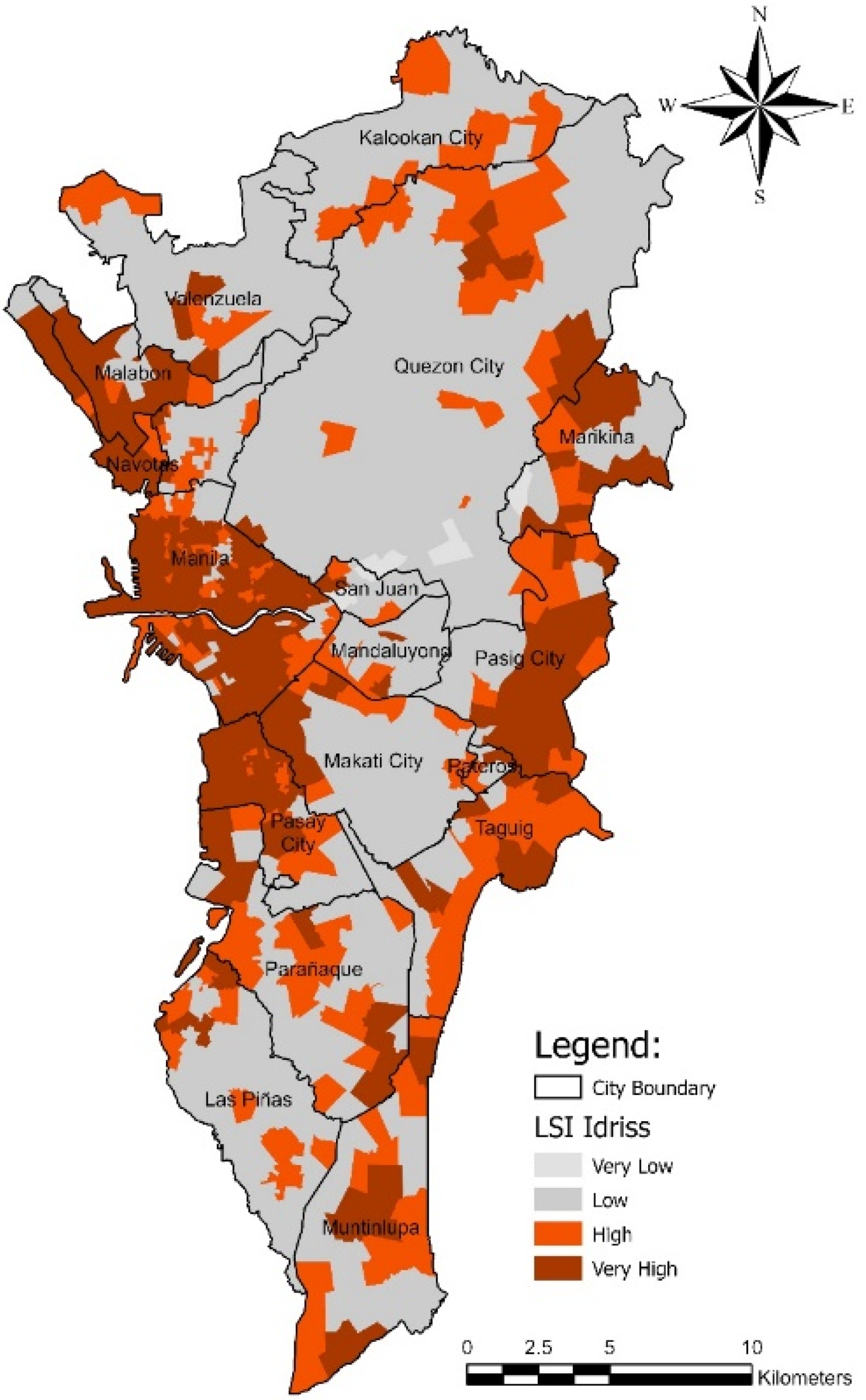
3.2. Case Study: Metro Manila, Philippines

This research will focus on Metro Manila, also known as the National Capital Region (NCR). The region consists of sixteen cities and one municipality and serves as a commercial, educational, and cultural center for the Philippines. Metro Manila is the most densely populated region in the country, with a population density of approximately 20,000 people per square kilometer as of 2021, with an estimated population of approximately 13 million people. Due to migration from other parts of the country in search of better economic opportunities, the population has increased rapidly.

In recent years, new residential and commercial developments have been constructed to meet the rising demand for housing and office space because of the population increase. For construction projects, a geotechnical investigation is necessary to determine the site’s suitability for proposed developments. Due to its high population density, rapid urbanization, and earthquake susceptibility, Metro Manila is an excellent location for a case study to determine the significant liquefaction susceptibility.

As shown in Figure 8, a total of 1656 geotechnical investigation data were collected from within and surrounding Metro Manila. Using GIS, the areas of each zone were then determined, and any areas larger than 1 km² were reduced through microzonation. This resulted in an increase from the original 1690 zones to a total of 2036 zones, shown in Figure 9. In addition, the centroids of each zone have been determined using GIS and are provided in latitude and longitude format.

Metro Manila’s susceptibility to liquefaction was evaluated in this study using the methodology developed by Idriss et al. [1]. This methodology employs the equation for the factor of safety (FS) against liquefaction, which is written in terms of the cyclic resistance ratio for earthquakes (CRR) and the cyclic stress ratio (CSR) resulting from the earthquake’s shaking. The CSR is the seismic demand placed on a soil layer and is computed using the peak horizontal acceleration (PGA) at the surface of the ground caused by the earthquake. As discussed in the previous section, the DSHA was employed to estimate PGA. DSHA involves calculating the distance from the source of the fault and the magnitude of the anticipated earthquake. Within the context of Metro Manila, it was discovered that the Marikina West Valley fault has a prominent presence. The cities of Quezon City, Marikina, Pasig, San Juan, Mandaluyong, Pateros, Makati, Taguig, Paranaque, and Muntinlupa are at risk if the fault line ruptures, as they all lie within 0–2 km of the fault line, shown in Figure 10. The NCR cities located farthest from the Marikina West Valley Fault are Malabon and Navotas.

In this study, a parametric analysis was performed to determine the evolution of peak ground acceleration (PGA) in Metro Manila for earthquakes with magnitudes ranging from 5.0 to 9.0. The Marikina West Valley Fault is a major contributor to seismic activity in Metro Manila and poses a significant threat of a magnitude 6 to 7.5 earthquake. This earthquake could cause a significant number of fatalities and injuries. In the National Capital Region,

Table 5. Range of PGA at different earthquake magnitudes in Metro Manila.

Magnitude	Range of Peak Ground Acceleration (PGA) Magnitude
	Minimum in g	Maximum in g
5.0	0.12	0.15
6.0	0.22	0.24
7.0	0.32	0.34
7.5	0.37	0.39

displays the range of peak ground acceleration at different earthquake magnitudes.

By conducting a parametric analysis and presenting the resulting data in Table 5, this study contributes to our understanding of the seismic hazards this region faces and emphasizes the significance of proactive risk management and disaster preparedness measures. A reference PGA map of Metro Manila at an expected magnitude 7.5 M earthquake is shown in Figure 11.

This study’s map of estimated peak ground acceleration (PGA) for Metro Manila is consistent with the results of a previous study by Dungca and Montejo (2022) [53]. In addition to assessing the amplification of seismic waves based on soil properties, their study produced a seismic hazard map for Metro Manila with a 10% probability of exceedance (POE). In this study, the PGA values for Metro Manila and other important geotechnical parameters were used to calculate the factor of safety (FS) against liquefaction. The probability of liquefaction (PL) was then calculated, and the resulting liquefaction severity index (LSI) was used to assess the liquefaction hazard of various zones within Metro Manila. As depicted in Figure 11, a liquefaction hazard assessment was conducted for an anticipated magnitude of 7.50 on the Marikina West Valley Fault, and a map was produced using the methodology developed by Idriss et al. (2004) [1]. This map provides vital information regarding the likelihood of liquefaction and associated risks in various areas of Metro Manila.

It is evident that the susceptibility of a layer to liquefaction is determined by its N-value, and layers with N-values greater than 30 are not considered susceptible to liquefaction, shown in Figure 12. In addition, the first 20 m of the investigated area in these cities consists of clayey soils that are non-liquefiable. The liquefaction severity index varies between various Metro Manila cities. There is a mixture of low, high, and very high values in Caloocan, Las Pinas, and Quezon City. Some cities on the Central Plateau have non-liquefiable areas due to the presence of sand in the shallow layers. However, the risk of liquefaction is greater in Makati, Mandaluyong, and San Juan near the west. In contrast, Marikina, Muntinlupa, Paranaque, Pasig, Pateros, Taguig, and Valenzuela have low, high, and extremely high liquefaction severity index values. The cities on both the Central Plateau and the Plain have a range of low, high, and extremely high liquefaction severity index values. Malabon, Manila, Navotas, and Pasay are, however, the most common locations with extremely high liquefaction severity index values. Consequently, coastal cities have an exceptionally high liquefaction severity index, making them more susceptible to liquefaction during earthquakes. The resulting liquefaction potential map concurs with local findings, which determined that the coastal and plateau cities of Metro Manila have the highest liquefaction potential.

3.3. Validation

To validate the model’s accuracy, data that were not utilized during training were used. Specifically, the unused data used for sample validation were located at 14.683126, 120.942226 (Latitude, Longitude) in Dampalit, Malabon City. The ground elevation was estimated to be 3 m as the initial estimated parameter for site-specific properties. With an accuracy rate of 83%, this estimate was found to be close to the USGS-obtained value of 2.5 m.

Estimating the depth of groundwater was also essential for geotechnical engineering, particularly in Metro Manila’s coastal regions, where the depth of groundwater is typically shallow. Both the estimated and collected data yielded a value of 1m, resulting in a 100 percent accuracy rate. The model framework permitted the estimation of several site-specific parameters, including the SPT N-value, USCS (soil type), liquid limit, and plastic limit of the target site. The accuracy of these estimates ranged between 75% and 86%, indicating that the estimated parameters and the collected data are in excellent agreement.

However, it was determined that the average accuracy of the N-value estimates was 84%, with some layers exhibiting low accuracy. This can be attributed to the tree model’s inability to account for erratic soil layer trends. This is applicable to USCS and Atterberg limits. In contrast, the accuracy of unit weight estimates varied between 87% and 95%.

With regard to the seismic behavior of the target location, the estimated peak ground acceleration was compared to the PHIVOLCS map of Metro Manila’s 1000-year return period for peak ground acceleration. This comparison was found to be 96% accurate, indicating a reliable estimate. In addition, both the estimated classification and the classification from the Metro Manila Earthquake Impact Reduction Study (MMEIRS) concur that the liquefaction classification for the target area is Very High. This is likely due to the target area’s proximity to the coast and the prevalence of sand layers.

4. Conclusions

In conclusion, the successful application of machine learning algorithms to estimate liquefaction susceptibility in the Metro Manila, Philippines study demonstrates the significance of incorporating geotechnical factors and sufficient data for accurate modeling. The study’s findings indicate that an increase in usable borehole data leads to improved model performance, as evidenced by the decrease in RMSE and the increase in R². These results highlight the importance of data in improving the accuracy of machine learning models and the potential of these algorithms to inform liquefaction risk assessments and mitigation efforts beyond the study area.

In addition, this research has demonstrated the practicality of using latitude and longitude as input variables to estimate site-specific characteristics such as ground elevation, groundwater elevation, soil type, and various soil properties. The highly positive correlation between the trained models for ground elevation, groundwater table elevation, SPT N-value, and fines content indicates a good fit with the data. Moreover, among competing models, the nearest neighbor model has demonstrated the highest level of accuracy in estimating the soil type for each layer.

Nonetheless, the study also uncovered a significant limitation in site-specific models. Due to the large number of variables, including spatial relationships, it is impossible to represent them with a single equation. Thus, these site-specific trained models are commonly known as black boxes. This limitation highlights the need for additional research to develop more interpretable models that can shed light on the mechanisms underlying the observed patterns.

In addition, a calibrated model represented by an equation was utilized in this study to determine various soil properties, such as liquefaction susceptibility and maximum surface ground acceleration (PGA). The linear model has demonstrated a highly significant positive correlation for PGA, and the estimated values fall within a reasonable range when compared to the findings of other studies. Nevertheless, the formula for estimating PGA is restricted to locations within a 100 km radius of seismic sources, even though the distance can exceed 100 km.

In addition, the comprehensive study on seismic activity in Metropolitan Manila, particularly on the Marikina West Valley Fault, has revealed alarming findings that pose an important danger to the safety and security of the area’s residents. The conducted parametric analysis to determine the development of peak ground acceleration for earthquakes ranging in magnitude from 5.0 to 9.0 resulted in a map of Metro Manila’s estimated PGA that is consistent with previous research, thereby bolstering the validity of the study’s findings.

In addition, the study’s calculations of probability of liquefaction (PL) and liquefaction severity index (LSI) for each layer, as well as the resulting liquefaction potential map, indicate that the coastal and plateau cities of Metro Manila have the highest liquefaction potential. This emphasizes the need for immediate action to mitigate the threat and safeguard the lives of area residents.

The validation process utilizing unused Dampalit, Malabon City data further demonstrates the high degree of accuracy of the model developed in the study, thereby enhancing confidence in the reliability of the model.

References

1. Youd, T.L.; Idriss, I.M. Liquefaction Resistance of Soils: Summary Report from the 1996 NCEER and 1998 NCEER/NSF Workshops on Evaluation of Liquefaction Resistance of Soils. J. Geotech. Geoenviron. Eng. 2001, 127, 297–313. [Google Scholar] [CrossRef]
2. Holzer, T.L.; Jayko, A.S.; Hauksson, E.; Fletcher, J.P.B.; Noce, T.E.; Bennett, M.J.; Dietel, C.M.; Hudnut, K.W. Liquefaction caused by the 2009 Olancha, California (USA), M5.2 earthquake. Eng. Geol. 2010, 116, 184–188. [Google Scholar] [CrossRef]
3. Muhammad, N.; Namdar, A.; Zakaria, I.B. Liquefaction mechanisms and mitigation-a review. Res. J. Appl. Sci. Eng. Technol. 2013, 5, 574–578. [Google Scholar] [CrossRef]
4. Juang, C.H.; Yang, S.H.; Yuan, H.; Fang, S.Y. Liquefaction in the Chi-Chi earthquake-effect of fines and capping non-liquefiable layers. Soils Found. 2005, 45, 89–101. [Google Scholar] [CrossRef]
5. Isobe, K.; Ohtsuka, S.; Nunokawa, H. Field investigation and model tests on differential settlement of houses due to liquefaction in the Niigata-ken Chuetsu-Oki earthquake of 2007. Soils Found. 2014, 54, 675–686. [Google Scholar] [CrossRef]
6. Sarah, D.; Soebowo, E. Liquefaction due to the 2006 Yogyakarta Earthquake: Field Occurrence and Geotechnical Analysis. Procedia Earth Planet. Sci. 2013, 6, 383–389. [Google Scholar] [CrossRef]
7. Marcuson, W.F. Definition of terms related to liquefaction. J. Geotech. Engrg. Div. 1978, 104, 1197–1200. [Google Scholar]
8. Beyzaei, C.Z.; Bray, J.D.; van Ballegooy, S.; Cubrinovski, M.; Bastin, S. Depositional environment effects on observed liquefaction performance in silt swamps during the Canterbury earthquake sequence. Soil Dyn. Earthq. Eng. 2018, 107, 303–321. [Google Scholar] [CrossRef]
9. Mojtahedzadeh, N.; Siddharthan, R. Estimating free field seismic settlement history in a saturated layered soil profile. Soil Dyn. Earthq. Eng. 2021, 150, 106937. [Google Scholar] [CrossRef]
10. Kteich, Z.; Labbé, P.; Javelaud, E.; Semblat, J.F.; Bennabi, A. Extended equivalent linear model (X-ELM) to assess liquefaction triggering: Application to the City of Urayasu during the 2011 Tohoku earthquake. Soils Found. 2019, 59, 750–763. [Google Scholar] [CrossRef]
11. Kang, G.C.; Chung, J.W.; Rogers, J.D. Re-calibrating the thresholds for the classification of liquefaction potential index based on the 2004 Niigata-ken Chuetsu earthquake. Eng. Geol. 2014, 169, 30–40. [Google Scholar] [CrossRef]
12. Wijewickreme, D.; Atukorala, U.D. Chapter 16 Ground improvement for mitigating liquefaction-induced geotechnical hazards. In Elsevier Geo-Engineering Book Series; Elsevier: Amsterdam, The Netherlands, 2005; Volume 3, pp. 447–489. [Google Scholar]
13. Venkata, N.; Kumar Velpuri, P. Factors Influencing the Microbial Calcium Carbonate Precipitation Performance in Sands; The University of Texas at Arlington: Arlington, TX, USA, 2015. [Google Scholar]
14. Karim, H.H. Evaluation of Some Geotechnical Properties and Liquefaction Potential from Seismic Parameters. Iraqi J. Civ. Eng. 2010, 6, 30–45. [Google Scholar]
15. Uy, E.E.S.; Adajar, M.A.Q.; Galupino, J.G. Utilization of Philippine gold mine tailings as a material for geopolymerization. Int. J. GEOMATE 2021, 21, 28–35. [Google Scholar]
16. Galupino, J.; Dungca, J. Machine learning models to generate a subsurface soil profile: A case of Makati City, Philippines. Int. J. GEOMATE 2022, 23, 57–64. [Google Scholar] [CrossRef]
17. Galupino, J.G.; Dungca, J.R. Quezon City soil profile reference. Int. J. GEOMATE 2019, 16, 48–54. [Google Scholar] [CrossRef]
18. Look, B. Handbook of Geotechnical Investigation and Design Tables; Taylor & Francis/Balkema: Leiden, The Netherlands, 2007; pp. 1–356. [Google Scholar]
19. Dungca, J.R.; Chua, R.A.D. Development of a probabilistic liquefaction potential map for Metro Manila. Int. J. GEOMATE 2016, 10, 1804–1809. [Google Scholar]
20. Peck, R.; Hanson, W.; Thornburn, T. Foundation Engineering, 2nd ed.; John Wiley & Sons: Hoboken, NJ, USA, 1974; Volume 2. [Google Scholar]
21. Geyin, M.; Maurer, B.W.; Christofferson, K. An AI driven, mechanistically grounded geospatial liquefaction model for rapid response and scenario planning. Soil Dyn. Earthq. Eng. 2022, 159, 107348. [Google Scholar] [CrossRef]
22. Ameratunga, J.; Sivakugan, N.; Das, B.M. Correlations of Soil and Rock Properties in Geotechnical Engineering; Springer: Berlin/Heidelberg, Germany, 2016. [Google Scholar]
23. Valverde-Palacios, I.; Valverde-Espinosa, I.; Irigaray, C.; Chacón, J. Geotechnical map of Holocene alluvial soil deposits in the metropolitan area of Granada (Spain): A GIS approach. Bull. Eng. Geol. Environ. 2014, 73, 177–192. [Google Scholar] [CrossRef]
24. Finn, W.D.L.; Dowling, J.; Ventura, C.E. Evaluating liquefaction potential and lateral spreading in a probabilistic ground motion environment. Soil Dyn. Earthq. Eng. 2016, 91, 202–208. [Google Scholar] [CrossRef]
25. Lee, D.H.; Ku, C.S.; Yuan, H. A study of the liquefaction risk potential at Yuanlin, Taiwan. Eng. Geol. 2004, 71, 97–117. [Google Scholar] [CrossRef]
26. Kim, H.S.; Kim, M.; Baise, L.G.; Kim, B. Local and regional evaluation of liquefaction potential index and liquefaction severity number for liquefaction-induced sand boils in pohang, South Korea. Soil Dyn. Earthq. Eng. 2021, 141, 106459. [Google Scholar] [CrossRef]
27. Dawson, K.M.; Baise, L.G. Three-dimensional liquefaction potential analysis using geostatistical interpolation. Soil Dyn. Earthq. Eng. 2005, 25, 369–381. [Google Scholar] [CrossRef]
28. Gajurel, A.; Chittoori, B.; Mukherjee, P.S.; Sadegh, M. Machine learning methods to map stabilizer effectiveness based on common soil properties. Transp. Geotech. 2021, 27, 100506. [Google Scholar] [CrossRef]
29. Dungca, J.R.; Galupino, J.G. Artificial neural network permeability modeling of soil blended with fly ash. Int. J. GEOMATE 2017, 12, 76–83. [Google Scholar] [CrossRef]
30. Pal, M.; Singh, N.K.; Tiwari, N.K. M5 model tree for pier scour prediction using field dataset. KSCE J. Civ. Eng. 2012, 16, 1079–1084. [Google Scholar] [CrossRef]
31. Ghani, S.; Kumari, S.; Bardhan, A. A novel liquefaction study for fine-grained soil using PCA-based hybrid soft computing models. Sādhanā 2021, 46, 113. [Google Scholar] [CrossRef]
32. Ghani, S.; Kumari, S.; Ahmad, S. Prediction of the Seismic Effect on Liquefaction Behavior of Fine-Grained Soils Using Artificial Intelligence-Based Hybridized Modeling. Arab. J. Sci. Eng. 2022, 47, 5411–5441. [Google Scholar] [CrossRef]
33. Ghani, S.; Kumari, S. Liquefaction behavior of Indo-Gangetic region using novel metaheuristic optimization algorithms coupled with artificial neural network. Nat. Hazards 2021, 111, 2995–3029. [Google Scholar] [CrossRef]
34. Uy, E.E.S.; Dadios, E.P.; Dungca, J.R. Preliminary assessment of liquefiable area in Ermita, Manila using genetic algorithm. In Proceedings of the 8th International Conference on Humanoid, Nanotechnology, Information Technology, Communication and Control, Environment and Management, HNICEM 2015, Cebu City, Philippines, 9–12 December 2015. [Google Scholar]
35. Wang, H.; Wang, X. Study of AI Based Methods for Characterization of Geotechnical Site Investigation Data; Ohio Department of Transportation, Office of Statewide Planning and Research: Columbus, OH, USA, 2020. [Google Scholar]
36. Ahmed, C.; Mohammed, A.; Tahir, A. Geostatistics of strength, modeling and GIS mapping of soil properties for residential purpose for Sulaimani City soils, Kurdistan Region, Iraq. Model. Earth Syst. Environ. 2020, 6, 879–893. [Google Scholar] [CrossRef]
37. Shi, C.; Wang, Y. Non-parametric machine learning methods for interpolation of spatially varying non-stationary and non-Gaussian geotechnical properties. Geosci. Front. 2021, 12, 339–350. [Google Scholar] [CrossRef]
38. University of Southern California. Uses of Geospatial Intelligence. 2021. Available online: https://gis.usc.edu/blog/4-uses-of-geospatial-intelligence/ (accessed on 10 May 2023).
39. Wojtkowska, M.; Kedzierski, M.; Delis, P. Validation of terrestrial laser scanning and artificial intelligence for measuring deformations of cultural heritage structures. Meas. J. Int. Meas. Confed. 2021, 167, 108291. [Google Scholar] [CrossRef]
40. Depellegrin, D.; Hansen, H.S.; Schrøder, L.; Bergström, L.; Romagnoni, G.; Steenbeek, J.; Gonçalves, M.; Carneiro, G.; Hammar, L.; Pålsson, J.; et al. Current status, advancements and development needs of geospatial decision support tools for marine spatial planning in European seas. Ocean Coast. Manag. 2021, 209, 105644. [Google Scholar] [CrossRef]
41. Tien Bui, D.; Nhu, V.H.; Hoang, N.D. Prediction of soil compression coefficient for urban housing project using novel integration machine learning approach of swarm intelligence and Multi-layer Perceptron Neural Network. Adv. Eng. Inform. 2018, 38, 593–604. [Google Scholar] [CrossRef]
42. Efthimiou, N.; Psomiadis, E.; Panagos, P. Fire severity and soil erosion susceptibility mapping using multi-temporal Earth Observation data: The case of Mati fatal wildfire in Eastern Attica, Greece. Catena 2020, 187, 104320. [Google Scholar] [CrossRef]
43. Azarakhsh, Z.; Azadbakht, M.; Matkan, A. Estimation, modeling, and prediction of land subsidence using Sentinel-1 time series in Tehran-Shahriar plain: A machine learning-based investigation. Remote Sens. Appl. Soc. Environ. 2022, 25, 100691. [Google Scholar] [CrossRef]
44. Meshesha, D.T.; Tsunekawa, A.; Haregeweyn, N. Determination of soil erodibility using fluid energy method and measurement of the eroded mass. Geoderma 2016, 284, 13–21. [Google Scholar] [CrossRef]
45. Naderpour, M.; Rizeei, H.M.; Khakzad, N.; Pradhan, B. Forest fire induced Natech risk assessment: A survey of geospatial technologies. Reliab. Eng. Syst. Saf. 2019, 191, 106558. [Google Scholar] [CrossRef]
46. Saraygord Afshari, S.; Enayatollahi, F.; Xu, X.; Liang, X. Machine learning-based methods in structural reliability analysis: A review. Reliab. Eng. Syst. Saf. 2022, 219, 108223. [Google Scholar] [CrossRef]
47. Bishop, C. Pattern Recognition and Machine Learning; EAI/Springer Innovations in Communication and Computing: New York, NY, USA, 2006. [Google Scholar]
48. Bowles, J.E. Foundation Analysis and Design. In Civil Engineering Materials; The McGraw-Hill Companies, Inc.: New York, NY, USA, 1997. [Google Scholar]
49. Puri, N.; Prasad, H.D.; Jain, A. Prediction of Geotechnical Parameters Using Machine Learning Techniques. Procedia Comput. Sci. 2018, 125, 509–517. [Google Scholar] [CrossRef]
50. Rahman, M. Foundation Design using Standard Penetration Test (SPT) N-value. Researchgate 2019, 5, 1–39. [Google Scholar]
51. Anbazhagan, P.; Uday, A.; Moustafa, S.S.R.; Al-Arifi, N.S.N. Correlation of densities with shear wave velocities and SPT N values. J. Geophys. Eng. 2016, 13, 320–341. [Google Scholar] [CrossRef]
52. Terzaghi, K.; Peck, R.; Mesr, G. Soil Mechanics in Engineering Practice; John Wiley & Sons, Inc.: Hoboken, NJ, USA, 1996. [Google Scholar]
53. Dungca, J.R.; Montejo, M.F.G. Metropolitan Manila Seismic Hazard Map Using Midorikawa & Hori Site Amplification Model. Int. J. Geomate 2022, 22, 92–99. [Google Scholar]
Figure 1. Modeling of site-specific properties.
Applsci 13 06549 g001
Figure 2. Modeling soil type using classification models.
Applsci 13 06549 g002
Figure 3. Modeling other site-specific geotechnical properties.
Applsci 13 06549 g003
Figure 4. Process in modeling the unit weight of a soil layer.
Applsci 13 06549 g004
Figure 5. Initial considerations in determining liquefiable and non-liquefiable soil layers.
Applsci 13 06549 g005
Figure 6. Classification of LSI.
Applsci 13 06549 g006
Figure 7. The case study, Metro Manila, Philippines.
Applsci 13 06549 g007
Figure 8. Locations of collected geotechnical investigation data.
Applsci 13 06549 g008
Figure 9. Microzonation of Metro Manila, Philippines.
Applsci 13 06549 g009
Figure 10. Distance of Metro Manila Zones from Marikina West Valley Fault.
Applsci 13 06549 g010
Figure 11. PGA map of Metro Manila at expected magnitude 7.5 M earthquake.
Applsci 13 06549 g011
Figure 12. LSI Map of Metro Manila, Philippines.
Applsci 13 06549 g012