Abstract
In order to solve the difficulties of dispatching the regional integrated energy system (RIES) under the operating conditions of multi-energy complementary mechanisms, as well as to achieve the purpose of economic operation and low carbon operation of the system, an optimal dispatching model of RIES, including demand response (DR) and an improved carbon trading mechanism (ICTM), is proposed. Firstly, a demand response model is established, the cooling, thermal, electricity, and gas load models under demand response are built, and then an improved customer satisfaction model is proposed based on the four demand response load models. In addition, since EV trips fit a normal distribution, the charging load of EVs is predicted using a Monte Carlo method and incorporated into RIES as a demand-side load; moreover, for EVs, an improved genetic algorithm is used to optimize EV charging, aiming to reduce the peak-to-valley difference; secondly, carbon emission quotas are provided for systems and EVs based on the baseline method and gratuitous allocation, and a carbon trading model is constructed based on carbon quotas and actual A carbon trading model for the system and EV is constructed based on the carbon allowances and actual carbon emissions; finally, four operation scenarios are set up in this paper, and the unit output scheme is developed with the objective of achieving the lowest total system operation cost and lowest carbon emissions. The four typical scenarios are solved using the MATLAB/CPLEX solver and compared for analysis. The simulation results show that an improved genetic algorithm for optimizing the ordered charging method of electric vehicle charging reduces the peak valley difference by 23.06%, and the total operation cost and carbon transaction cost are reduced by 16.13% and 83.10%, respectively, which can provide a reference for the environmental protection and economic dispatch of RIES.
1. Introduction
In today‘s world, problems such as energy shortages, environmental pollution, and ecological deterioration are gradually deepening, and the contradiction between energy supply and demand is becoming increasingly prominent. Therefore, it is urgent to improve energy efficiency and promote energy transformation and upgrading [1,2]. With the widespread use of various renewable energy generation technologies, RIES is of great significance in improving energy utilization efficiency, achieving complementary and coupled operation between various energy sources, and promoting China’s energy conservation and emission reduction strategic goals [3]. It will play a more important role in the energy system over time.
For the last few years, some scholars from home and abroad have conducted some studies about the RIES system. The Regional Integrated Energy System achieves complementary synergy and scientific scheduling among regional energy sources by organically combining multiple energy sources such as electricity, heat, and cooling with energy demand-side systems. Currently, the Integrated Energy System (IES) takes Combined Heat and Power (CHP) as its core and uses it as a platform to link regional energy sources with energy storage technology [4]. Carbon trading, also known as carbon emissions trading, is a trading mechanism that establishes legal carbon emissions rights and allows emitters to trade them on the market to achieve emission reduction goals. In [5], the actual output of the generator set was used as the standard to allocate the initial carbon emission right for the system for free, and the actual carbon emission is included to calculate the carbon transaction cost, which effectively improves the environmental protection and low carbon of the system but does not consider the user’s demand response. In [6], the price elasticity matrix is introduced to describe demand response behavior, and the effectiveness of DR in alleviating the peaking pressure of the system was analyzed, but low carbon was not guaranteed. In [7], the electric load models under DR were built in light of the price elasticity matrix method. Furthermore, based on the fuzziness and delay of the user’s thermal perception, the thermal load DR model was established, and it was verified that the model has a great impact on energy efficiency. However, the model did not consider carbon trading, cooling, or gas loads under DR. In [8], an optimal operation model of a multi-energy complementary cogeneration microgrid, including a demand response model on the demand side, is established, but the carbon trading mechanism and the interaction between power energy and gas energy are not considered. In [9], a CCHP microgrid model incorporating integrated demand response and dealing with the randomness of new energy output in the microgrid by scenario method was raised. In [10], the integrated demand response on the residential side based on micro CHP units was studied; however, the two did not consider the carbon trading mechanism and did not connect the CCHP microgrid considering demand response to the bulk power grid. In [11], the total operating cost and wind and light abandoning quantity of the system under different electrical and thermal load comfort levels are compared to achieve multi-energy complementarity, reduce operating costs, and improve new energy consumption on the basis of ensuring user comfort levels. However, the electric load DR only simplified the modeling of interruptible and moveable loads without considering the thermal load DR. In [12], considering the price transmission mechanism of the electricity market and carbon trading market, the electricity generation of renewable energy such as wind and light was converted into emission reduction, and a comprehensive demand-side response scheme of the multi-energy system, including the operation of cold, heat, and power cogeneration units and the control strategy of battery storage, was put forward to realize the economic operation of the multi-energy system in the park. However, the fine model of the load side has not been constructed. In [13], a peak load management model (PLM) was proposed, which can combine the driving time and driving position of the electric vehicle to schedule the charging and discharging service of the electric vehicle according to its load demand. In [14,15,16], it was proposed that the introduction of a carbon trading mechanism, which optimizes system resource allocation and promotes energy conservation and emission reduction. Energy conservation and emission reduction can make carbon emissions dispatchable resources with economic value. In [17,18], considering that DR can tap the potential of the energy side and achieve low-carbon economic operation of the system. In [19], a load prediction model based on momentary charging probability was proposed by establishing a probabilistic model of the factors influencing charging load prediction using probabilistic statistics and Monte Carlo simulation methods. In [20], the use of transformation matrices was proposed to predict the hourly charging rate of EVs, and simulations were performed using transformation matrices in specific regions. Monte Carlo methods were used to provide statistical results, but the above only provided a single prediction for EVs.
In summary, the current integrated energy system does not consider the thermal and cold electrical models and carbon trading mechanism under DR at the same time, and in the past, only a single load forecast for electric vehicles was made and the impact of electric vehicle load on the access system was ignored. In this paper, an optimal scheduling model of an integrated energy system with EV considering DR and carbon trading mechanisms is proposed. Firstly, the demand response model is analyzed to obtain the load reduction and transferable load models, and the cold, thermal, electricity, and gas load models under DR are refined at the same time. Furthermore, based on the baseline method and the free allocation method, the carbon emission quota is provided to the system to construct the carbon trading mechanism, which includes the system carbon trading mechanism and the separate electric vehicle carbon trading mechanism. The Monte Carlo method is used to predict the daily load of electric vehicles and count them into the power grid. The system aims to minimize the total operating cost. The results show that the total operation cost and carbon transaction cost of the proposed model are reduced by 16.13% and 83.10%, respectively, and the system operation cost is effectively reduced by considering the economy and low carbon.
2. RIES Model with DR and ICTM
2.1. RIES Structure
RIES, composed of various energy forms, conversion equipment, and coupling equipment, is able to satisfy the demands of the users, including electricity, heat, cold, gas, and other load demands. Furthermore, the system improves energy utilization efficiency, fulfills the user’s various energy needs, and ensures a continuous and reliable energy supply. The RIES structure is illustrated in Figure 1.
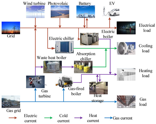
Figure 1.
RIES structure.
2.2. DR Model
DR can be defined as a behavior where users alter their consumption patterns according to the level of real-time electricity prices or the incentive mechanism. It can not only solve energy demand and reduce production costs, but also cut down the investment cost of generating units and have a nice improvement on power system dependability. The DR model can be classified into price-based demand response and incentive demand response based on response characteristics [21,22,23]. In this paper, the price of electricity varies at different times, which belongs to the price demand response model and can achieve the effect of peak-load shifting. Based on the difference in the sensitivity of different loads to the same electricity price change signal, the price-based demand response load can be classified into two categories: the curtailable load (CL), that is, whether the load is reduced by the electricity price change; and the shiftable load (SL), which changes its own demand according to the electricity price signal and can guide users to transfer the demand from the peak power consumption period to the flat valley period.
- Translatable load
The Translatable load model can be represented as a price demand elasticity matrix, where the electricity price of the load at time m to time n, that is, the mth row and nth column element a (m, n) in the elasticity matrix A (m, n) [24], is defined as:
The change of the translatable load at time m after DR can be given by the CL price demand elasticity matrix as:
- 2.
- Shiftable load
Similarly, the SL variation at time t after DR can be expressed as:
where is the initial transferable load at time m; the diagonal matrix is the SL price demand elasticity matrix.
Under the incentive of electricity price, the power load DR modeling can be shown as [25]:
where ,, , and are the cold, thermal, electric, and gas loads before demand response; , , and represent the variation of cold, thermal, electricity, and gas loads under demand response.
2.3. Structure of the Improved Carbon Trading Mechanism
The CTM can be defined as a mechanism for trading carbon emission rights on carbon exchanges, which boosts carbon emission reduction effectively. The determination of carbon emissions is a key step in the carbon emission mechanism. This paper is based on the baseline method and uses the free distribution method to provide carbon emission quotas for the system. Previously, carbon trading was mostly focused on the power grid itself, and the paper introduced a carbon trading model for electric vehicles. The principle of the carbon trading mechanism is shown in Figure 2.
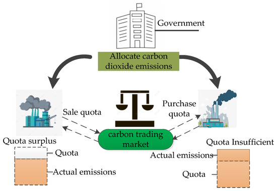
Figure 2.
Principles of the carbon trading mechanism.
For the RIES model set up here, the carbon emissions come from the purchase of electricity, gas turbines (GT), and gas boilers (GB) from the superior power grid. GT generates electricity and produces heat, while GB only produces heat. The carbon permits of RIES at time t are as follows:
where is the regional carbon emission allocation per unit of electricity, which is 0.065 kg/kWh; is the conversion factor of electricity, which is 6 [26].
The actual carbon emission is the total of GT and GB. In line with the carbon emission factor method, this paper considers that the carbon emission of the unit is in direct proportion to its contribution, and if this paper considers that the superior power purchase comes from the gas unit power generation, then the actual carbon emission is described as:
where and are carbon emission factors for GT and GB, which both are 0.102 kg/kW; is 0.728 kg/kW [27].
In order to encourage the system to actively participate in carbon exchanges, the carbon trading strategy constructed in this paper is as follows: users can trade carbon emission quotas themselves, that is, selling when they are more and buying when they are less. The carbon transaction cost at time t is given as:
where is carbon’s price.
For electric vehicles, the emission reduction saved by electric vehicles driving the same distance as fuel vehicles is taken as the carbon quota. Therefore, this paper proposes a carbon trading model for electric vehicles. Profit from selling carbon quotas on electric cars is shown in Equations (8) and (9).
where is the output of a GT in period t; G is the total number of GT; is the carbon emission quota of electric vehicles in period t; is the mileage that can be driven per unit power of the electric vehicle, which is 5 km in this paper; is the carbon emissions when the fuel vehicle travels 1 km, which is 0.197 kg/km in this paper; is the marginal carbon emission factor of electric vehicles; is the active power output of clean energy at time t; is the profit of selling carbon quota for electric vehicles in period t; is the selling price of electric vehicle carbon quota.
2.4. Improved User Satisfaction
According to [28], the calculation method for user satisfaction is given as:
In this paper, considering the user’s multiple energy load demands, the user satisfaction is combined with the cold, thermal, electricity, and gas load responses, and the user satisfaction with energy supply is fully considered. An improved calculation model for user satisfaction is proposed. The is expressed as,
represents the user’s satisfaction, which is a number between 0 and 1.
3. Model of Main Equipment
3.1. Gas Turbine
The output power model of the gas turbine (GT) is described as Equations (12) and (13) [29]:
where denotes the output electric power of GT; is the power generation efficiency of a gas turbine.
The gas consumption of the GT is shown in the following equation,
where represents the GT output heat power; represents the heat loss efficiency, and the value is 0.1; is the calorific value of natural gas, and its value is 9.7 kWh/m3.
3.2. Waste Heat Boilers and Electric Boilers
The output power models of waste heat boilers (WHB) and electric boilers (EB) are shown as:
where represents the output electric power of WHB; is the power generation efficiency of WHB; and respectively represent the input and output power of an electric boiler.
3.3. Gas Boiler
When the output of WHB and EB is less than the thermal demand of the RIES, it will be compensated by GB. The model of GB can be given as:
where represents the efficiency of a gas turbine, which is 0.9.
3.4. Electric Chiller and Absorption Chiller
The output model of an electric chiller (EC) can be expressed as:
Where and denote the input and output power of the refrigerator, respectively; is 4, indicating the refrigeration coefficient.
The output model of the absorption chiller (AC) can be given as:
where and represent the input and output power of the absorption refrigerator, respectively; is the energy consumption ratio, and the value is 1.2.
3.5. Electric Vehicles
Electric vehicles can participate in charging scheduling when they are parked; thus, their parking time directly determines the length of charging time. At present, the charging mode of electric vehicles can be approximated as constant power charging [25]. According to the data obtained from the research survey of relevant departments in the US Department of Transport, the user’s last returnable time tτ on the day obeys the normal distribution and can be described as [30]:
where and represent the mean and variance, which are 17.6 and 3.4, respectively.
According to the findings of the US Department of Transportation on the travel of electric vehicle users, the daily mileage L of electric vehicles obeys the logarithmic normal distribution L-log (μl, σl) and can be shown as:
where and are 3.2 and 0.88, respectively.
The daily mileage L and charging time T of electric vehicles are in accordance with the following function:
where E is 0.5 kWh/km; is 3 kW; is 0.9.
4. Optimal Operation Model of the RIES System
4.1. Objective Function
The RIES optimal operation model in account of DR and EV under the CTM aims to achieve the best economy of the whole system under the precondition of the following constraints. The objective function of RIES can be indicated as:
where F is the overall cost of the RIES optimization model; and are the interaction costs of the RIES system with the outside world; is carbon transaction cost; is the total running and maintaining cost.
4.1.1. Energy Interaction Cost
The Cbuy includes the power transaction cost between the system and the bulk grid and the gas transaction cost between the system and the gas network. stands for profit from the sale of excess electricity. If the electric energy provided by each power equipment in RIES is not enough to fulfill its own power requirements, the system needs to acquire it from the bulk grid; if not, excess energy is sold. Similarly, the gas turbine and gas boiler in the system need to consume gas and produce electricity, so the RIES has to acquire gas from the gas network to maintain the system’s operation. Therefore, the cost of purchasing and selling energy can be expressed as:
where and are purchase and sale prices of electricity at time t, respectively; and is the gas price.
4.1.2. Carbon Transaction Cost
consists of the carbon transaction cost of RIES units and the carbon transaction cost of the system’s interaction with the grid; that is, the carbon transaction cost is the sum of the two costs and can be shown as:
4.1.3. Operation and Maintenance Cost
Operation and maintenance cost can be described as:
where is the operational maintenance factor; is the output value of each unit at time t; is the start-stop cost of GT; is the number of GT starts.
4.1.4. Environmental Benefit Cost
The environmental benefit cost is shown as:
where means the jth pollution generated by the ith distributed power source per unit power; is the unit cost of treating the jth pollutant.
4.2. Constraint Conditions
The RIES set up in this paper includes cold energy flow, thermal energy flow, electric energy flow, and gas energy flow, all of which need to meet energy constraints.
The cold energy flow constraint is shown as,
where is the cooling load before DR; is cold load variation between 0 and 220.
The heat energy flow constraint can be expressed as:
where is the heating load before DR; is heat load variation between 0 and 160.
The electrical energy flow constraint can be given as:
where denotes the electrical load before DR; is the electrical load variation between 0 and 150.
The gas energy flow constraint can be described as:
where represents the air load before DR; is the gas load variation between 0 and 30.
The constraints of the energy storage device are as follows: the energy storage device includes a battery (BAT) and a heat storage device (HS). The charge level of the energy storage device is related to its operating state [31]. The charge level of the device [32] is shown as:
where SOC represents the charge level; is the power of the energy storage device; denotes the static state variable of the device; and severally stands for the charging and discharging of the equipment.
The changed electric energy transfer constraint can be illustrated as [33]:
where is 0.2, representing the total power transfer limit; is the changed electric energy limit in time t, and the value is 150; , , are the totally changed loads of the original peak period, normal period, and low period, respectively; , , are the total loads of the original peak period, normal period, and low period, respectively; is the amount of electrical load changing in the t period.
4.3. Solution Method
As the problem in this paper is a mixed integer linear programming problem, the model is solved by MATLAB/CPLEX. Firstly, the DR model and the carbon trading mechanism are analyzed, and the cooling, thermal, electricity, and gas load models under the DR and the carbon trading mechanism model are established, while the unit parameters are input; next, the cooling, thermal, electricity, and gas load data of the system and the wind power output and PV output data are input, and the load curves are obtained. Based on the DR model, the load curves after the demand-side response are obtained, and the wind power output and PV output curves of the system are obtained; then, the daily load input RIES of the electric vehicle is predicted, and the load curves are obtained according to the Monte Carlo method. Finally, under the condition of satisfying the load balance constraint and unit power constraint, the unit output case and unit switching case under the minimum total cost of operation are solved and obtained with the objective of minimizing the total cost of operation of the system. The program flow chart is shown in Figure 3.
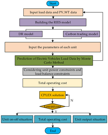
Figure 3.
RIES optimal solution flow chart.
5. Example Analysis
5.1. Data
This paper regards the combined cooling, thermal, electrical, and gas systems of a data center in Beijing as the research object and takes 24 h as a scheduling cycle, whose scheduling interval is one hour. The RIES system data is the load data of 300 electric vehicles obtained through the Monte Carlo method. According to the relevant load data for the daily operation of the system, the daily load curve is shown in Figure 4a. The daily load curve includes cooling load, thermal load, electric load, and gas load. As shown in the graph, the maximum daily demand of the four loads is about 1050 kW, 1580 kW, 1700 kW, and 380 kW, respectively. Based on the output power data of WT and PV, the output power of WT and PV can be obtained, as shown in Figure 4b. The main equipment parameter values in the RIES are shown in Table 1.
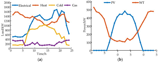
Figure 4.
The daily load curve and the output power data of WT and PV: (a) the daily load curve; (b) the output power data of WT and PV.

Table 1.
The main equipment parameter values.
5.2. Electric Vehicle Load
5.2.1. Monte Carlo Method
In this paper, the electric vehicle is introduced into the RIES. It is assumed that the number of electric vehicles is 300 or 400, and the charging behavior simulation is carried out. The electric vehicle starts to charge at a constant power rate after the last return until the state of charge reaches 100%. During the period, the electric vehicle adopts the slow charging mode, which is 3 kW, the charging efficiency ηe is 0.9, and the power consumption per kilometer E is 0.5 kW h/km. According to Equations (19) and (20), the probability density distribution of the daily driving mileage of users and the probability density distribution of the user’s last return time are shown in Figure 5a,b, respectively.
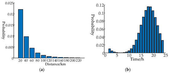
Figure 5.
The probability density distribution of daily driving mileage of users: (a) the probability density distribution of daily driving mileage of users; (b) the probability density distribution of the user’s last return time.
Figure 6 shows the Monte Carlo simulation of electric vehicle disorderly charging has a large peak-valley difference, which is easy to cause fluctuations in the power grid, and users are also charging during their noon-out hours. According to user habits, charging is usually performed from 17:00 to 8:00 the next day. Therefore, an improved genetic algorithm is considered to optimize the charging power of EVs to ensure orderly charging. The time-sharing pricing strategy aims to reduce charging costs and minimize peak-to-valley differences.
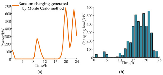
Figure 6.
Random charging by Monte Carlo method: (a) 400 electrical vehicles; (b) 300 electrical vehicles.
5.2.2. Improved Genetic Algorithm
Compared with the traditional genetic algorithm based on roulette wheel selection, the improved genetic algorithm has a faster convergence speed. Its basic idea is to establish an elite population based on the fitness of the previous generation population. In the selection process for the new generation, the elite population is used to replace the individuals with low fitness in the population.
In order to ensure that the algorithm is not limited to the local optimum as early as possible, the crossover and mutation rates are appropriately modified during the genetic process. k is the number of iterations, kk is the algebra that achieves continuous and constant optimal solution, and M is the maximum number of iterations that maintain continuous and constant optimal solution. That is to say, once the optimal solution remains unchanged during the iteration process and reaches generation M, the mutation and crossover rates are modified. The improved genetic algorithm flow is shown in Figure 7.
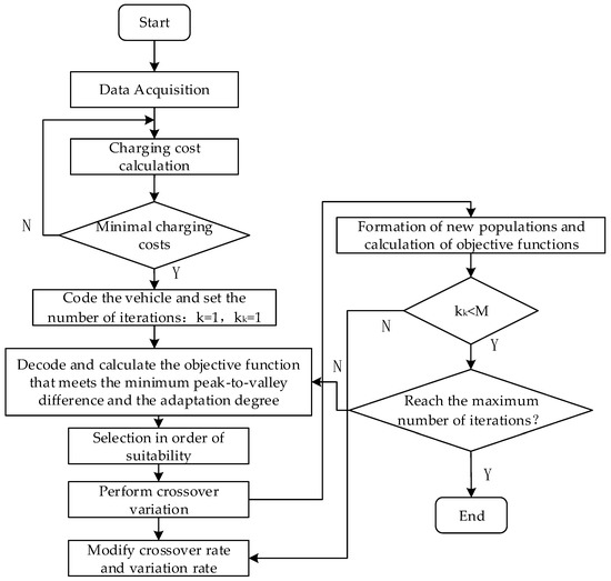
Figure 7.
Improved genetic algorithm flow.
Figure 8 shows that, under the premise of meeting the charging needs of users, orderly charging can reduce the peak-valley difference compared to disordered charging and achieve a certain degree of “peak shaving and valley filling”. The peak-to-valley difference has decreased by 23.08%, achieving stable operation of the power grid.
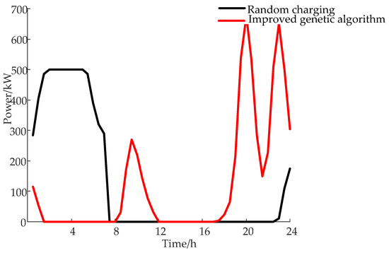
Figure 8.
The comparison between random charging and order charging of EVs.
5.3. Result Analysis
In this paper, a day is divided into three periods: peak, flat, and valley periods. The price of the system running in the three periods is different from that of the superior power grid. In order to make the transaction cost lower, the system needs to meet the low load required in the peak period and the peak load of user demand in the low period. The model proposed in this paper can achieve peak-cutting and low-filling and reduce the load transaction cost for users.
In order to verify the effectiveness and rationality of the optimal scheduling model of the RIES system considering demand response under the carbon trading mechanism proposed in this paper, RIES is set up to run in the following four modes, as shown in Table 2, and the electricity is shown in Table 3. The pollutant emission factor and pollutant treatment cost are shown in Table 4.
Table 2.
System operational.
Table 3.
Time-of-use electricity prices.
Table 4.
Pollutant discharge coefficient and pollution control cost.
When RIES is running in model 4, the electricity, cold, heat, and gas loads after demand response and the original load are shown in Figure 9a–d; besides, Figure 10a–d shows the output of each equipment under the conditions of electricity, heat, cold, and gas balance.
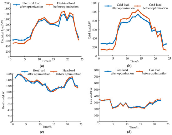
Figure 9.
Load comparison before and after DR: (a) electrical load; (b) cold load; (c) heat load; and (d) gas load.
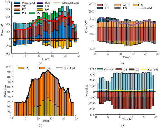
Figure 10.
The load balance under model 4: (a) electrical load; (b) heat load; (c) cold load; and (d) gas load.
Figure 9 shows the comparison curves of user-side electric, cold, heat, and gas loads before and after DR. After considering the DR, due to the response of the load to the electricity price, the load transfer cost is lower than the energy purchase cost in the two periods of 9:00–12:00 and 19:00–22:00 when the electricity price is higher, so the system chooses the load to be transferred to the low-price period, thus forming the trend of load peak load shifting. The peak value of the electric load before DR is 1690 kW and the valley value is 490 kW, while the peak value after DR is 1655 kW and the valley value is 635 kW. The peak-valley difference of the electric load is relatively reduced by 10.87%; besides, the peak value of the heat load before DR is 1584 kW and the valley value is 1008 kW, but the peak and valley values are 1586 kW and 1066 kW, respectively, under the DR strategy, and the difference between peak and valley of the heat load decreases by 3.61%. The peak value of the cooling load before DR is 1040 kW, and the valley value is 130 kW. However, under the DR strategy, the peak and valley values are 938 kW and 268 kW, respectively, and the peak and valley difference is relatively reduced by 12.65%; meanwhile, the peak-valley values of the exergy load before DR were 353 kW and 120 kW, respectively, while the peak-valley values after DR were 342 kW and 135 kW, respectively; that is, the peak-valley difference decreased by 12.29%. It follows that the fluctuation of cold, heat, electricity, and gas loads has also been effectively suppressed after considering DR, which verifies the optimization effect of demand response on cold, heat, electricity, and gas loads. At the same time, energy storage equipment can also play a role in peak chopping and valley filling according to the real-time demand response of the system. It can be seen that considering the demand response of cooling, heating, and power loads can effectively reduce the fluctuation of the load curve and improve the economy and environmental protection of the RIES system.
The optimization results shown in Table 5 are the daily operating costs of the system. According to Table 5, compared with scenario 1, the total cost of scenario 2 considering the demand response strategy is reduced by 1949.69 yuan, which is a decrease of 6.12%; carbon transaction costs are decreased by 6.28%; and the purchase cost is decreased by 6.80%. At the same time, the carbon emissions are decreased by 1449.65 kg, which indicates that the demand response is achieved through the transfer of load reduction, i.e., the peak load is transferred to the low, reducing the system’s electricity transaction costs, and this promotes the economic operation of the system. The total cost of scenario 3 considering the carbon trading mechanism is decreased by 3853.15 yuan, which is a decrease of 12.10%; the carbon transaction cost is reduced by 1231.64 yuan, which is 80.50%; the energy purchase cost is reduced by 12.36%; and the carbon emission is reduced by 2708.80 kg compared to scenario 1. This indicates that the carbon trading mechanism proposed in this paper makes the initial carbon emission quota owned by the system offset part of the carbon transaction cost, so that the carbon transaction cost of the system can be greatly reduced. At the same time, it shows that the carbon trading mechanism promotes the reduction of carbon emissions and has a good effect on the low-carbon operation of the system. In scenario 4, which considers both demand response and carbon trading strategies, the total cost of the system is reduced by 5137.63 yuan, or 16.13%; at the same time, compared with only the demand response strategy and only the carbon trading mechanism, the total cost is 10.66% and 4.59% lower, respectively. In addition, carbon trading costs decreased by 1271.43 yuan, which is 83.10%. At the same time, they are 81.97% and 13.34% lower than scene 2 and scene 3. The energy purchase cost decreased by 14.48%, and carbon emissions decreased by 5420.58 kg. It can be seen that considering demand response and carbon trading mechanisms can obtain better total cost, lower carbon transaction cost, and lower carbon emissions than a single strategy, so that the system operation can achieve both economy and low carbon. This is because the demand response strategy can transfer the load from the high electricity price period to the low electricity price period to reduce the energy trading volume between the system and the power grid and thus reduce the system purchase cost. The carbon trading mechanism allows the system to have an initial carbon allowance to offset the cost of carbon emissions, thereby reducing carbon emissions and carbon trading costs, resulting in a lower total cost of RIES operations and lower carbon emissions while being both economic and low-carbon.
Table 5.
Daily operating costs.
6. Conclusions
In this paper, an optimal operation model of RIES considering demand response under the carbon trading mechanism is established. Through the research on the RIES system of a data center in Beijing, the EV, carbon trading mechanism, and demand response strategy are introduced, and the relationship between them is considered. It is proven that the carbon trading mechanism and demand response can achieve comprehensive optimization of the economy and low carbon emissions in RIES. The specific conclusions are as follows:
- Under the carbon trading mechanism, considering the demand response, it not only shifts the peak load to the valley period, reduces the load energy consumption, and realizes the role of peak regulation and valley filling, but also realizes the mutual substitution, coupling, and smoothing of the load curves of electric energy and thermal energy, cold energy, and gas energy at the user side, and the shift of peak load to valley load greatly reduces the system energy consumption cost.
- The improved genetic algorithm is used to optimize the orderly charging method of EV charging, reducing the peak-to-valley difference by 23.06%, which can reduce the impact of excessive EV load on the system and achieve stable grid operation.
- The total operating cost of the RIES system with demand response considered decreased by 6.20% compared to the RIES without demand response considered; the total operating cost of the RIES with demand response considered decreased by 10.47%; and the overall cost of the RIES with demand response considered under the carbon trading mechanism proposed in this paper decreased by 16.13%, indicating that the economy of the system was greatly improved and the operating cost savings were achieved.
- The RIES system considering demand response reduces the carbon trading cost by 6.28% compared to the RIES without consideration and reduces the carbon trading cost of the grid by 80.5% compared to the RIES with consideration of the carbon trading mechanism. The RIES system considering demand response under the carbon trading mechanism proposed in this paper reduces the carbon trading cost by 83.10%, indicating that the environmental friendliness of the system is improved, which facilitates the reduction of carbon emissions and achieves the purpose of a low-carbon system.
In the next studies, the intention is to introduce electrical-to-gas technology into the system, refine the electrical-to-gas technology, and enhance the electrical coupling effect.
Author Contributions
Conceptualization, Z.L.; methodology, Z.L.; software, Y.Z. and Z.L.; validation, Z.L. and Y.Z.; formal analysis, Z.L. and Y.Z.; investigation, Y.W. and L.L.; data curation, Z.L. and Y.Z.; writing—original draft preparation, Z.L. and Y.Z.; writing—review and editing, Z.L. and Y.Z.; visualization, Z.L.; supervision, Y.W. and L.L.; project administration, Y.Z. and Y.W. All authors have read and agreed to the published version of the manuscript.
Funding
The Open Research Fund of Guangxi Key Laboratory of Building New Energy and Energy Conservation (Gui Keneng 17-J-21-4).
Institutional Review Board Statement
Not applicable.
Informed Consent Statement
Not applicable.
Data Availability Statement
Not applicable.
Conflicts of Interest
The authors declare no conflict of interest.
Nomenclature
| WT | Wind turbine. |
| PV | Photovoltaics. |
| EV | Electric vehicle. |
| GT | Gas turbine. |
| GB | Gas-fired boiler. |
| EB | Electric boiler. |
| WHB | Waste heat boiler. |
| AC | Absorption chiller. |
| EC | Electric chiller. |
| The load variation at moment m after DR. | |
| Initial load. | |
| Electricity price variation at time n after DR. | |
| The initial price at time n. | |
| Initial load reduced at time m. | |
| Electricity price at time n. | |
| The CL price demand elasticity matrix and the SL price demand elasticity matrix. | |
| The thermal and electrical power of the gas turbine at time t; the thermal power of the gas boiler at time t. | |
| Energy trading with the grid. | |
| Output thermal power of an electric boiler; Minimum and maximum output power of an electric boiler. | |
| Heat power of waste heat boilers and gas-fired boilers; the minimum and maximum output power of the gas turbine. | |
| The input of a gas boiler. | |
| The input and output power of the electric refrigerator; the minimum and maximum input power of the electric refrigerator. | |
| The input and output of the electric chiller; the minimum and maximum output of the electric chiller. | |
| The amount of electricity and gas purchased at the time t. | |
| Power generation and consumption of each piece of equipment; user electrical load demand. | |
| Heat release and heat storage power of the heat storage tank. |
References
- Li, P.; Wang, Z.X.; Yang, W.H.; Liu, H.T.; Yin, Y.X.; Wang, J.H.; Guo, T.Y. Hierarchically partitioned coordinated operation of distributed integrated energy system based on a master-slave game. Energy 2021, 214, 119006. [Google Scholar] [CrossRef]
- Zhou, Y.H.; Ge, F.; Dai, G.; Yang, Q.B.; Zhu, H.; Youssefi, N. Modified Arithmetic Optimization Algorithm: A new Approach for Optimum Modeling of the CCHP system. J. Electr. Eng. Technol 2022, 17, 3223–3240. [Google Scholar] [CrossRef]
- Li, P.; Zhang, F.; Ma, X.Y.; Yao, S.J.; Wu, Y.H.; Yang, P.; Zhao, Z.L.; Lai, L.L. Operation Cost Optimization Method of Regional Integrated Energy System in Electricity Market Environment Considering Uncertainty. J. Mod. Power Syst. Clean Energy 2023, 11, 368–380. [Google Scholar] [CrossRef]
- Wang, Y.L.; Wang, Y.D.; Huang, Y.J.; Yu, H.Y.; Du, R.T.; Zhang, F.L.; Zhang, F.W.; Zhu, J.R. Optimal Scheduling of the Regional Integrated Energy System Considering Economy and Environment. IEEE Trans. Sustain. Energy 2019, 10, 1939–1949. [Google Scholar] [CrossRef]
- Sun, P.R.; Hao, X.J.; Wang, J.; Shen, D.; Tian, L. Low-carbon economic operation for integrated energy system considering carbon trading mechanism. Energy Sci. Eng. 2021, 9, 2064–2078. [Google Scholar] [CrossRef]
- Cui, Y.; Xiu, Z.J.; Liu, C. Dual level optimal dispatch of power system considering demand response and pricing strategy on deep peak regulation. Proc. IEEE 2021, 41, 4403–4415. [Google Scholar]
- Kong, X.Y.; Sun, F.Y.; Huo, X.X.; Li, X.; Shen, Y. Hierarchical optimal scheduling method of heat-electricity integrated energy system based on Power Internet of Things. Energy 2020, 210, 118590. [Google Scholar] [CrossRef]
- Gong, X.; Li, F.; Sun, B. Collaborative Optimization of Multi-Energy Com-plementary Combined Colling, Heating, and Power Systems Considering Schedulable Loads. Energies 2020, 13, 918. [Google Scholar] [CrossRef]
- Jiang, Z.Q.; Ai, Q.; Hao, R. Integrated Demand Response Mechanism for Industrial Energy System Based on Multi-Energy Interaction. IEEE Access 2019, 7, 66336–66346. [Google Scholar] [CrossRef]
- Michiel, H.W.; Negenborn, R.R.; Schutter, B.D. Demand Response With Micro-CHP Systems. Proc. IEEE 2011, 99, 200–213. [Google Scholar]
- Zhao, H.P.; Miao, S.H.; Li, C. Research on Optimal Operation Strategy for Park-level Integrated Energy System Considering Cold-heat-electric Demand Coupling Response Characteristics. Proc. CSEE 2022, 42, 573–589. [Google Scholar]
- Yang, H.Z.; Li, M.L.; Jiang, Z.Y. Optimal Operation of Regional Integrated Energy System Considering Demand Side Heating Loads Response. Power Syst. Protec. Cont. 2020, 48, 30–37. [Google Scholar]
- Said, D.; Mouftah, H.T. A Novel Electric Vehicles Charging/Discharging Management Protocol Based on Queuing Model. IEEE Trans. Intell. Veh. 2020, 5, 100–111. [Google Scholar] [CrossRef]
- Liu, H.; Zhao, M.X.; Ge, S.Y. Sequential Power Flow Calculation of Power-heat Integrated Energy System Based on Refined Heat Network Model. Auto. Electr. Power Syst. 2021, 45, 63–72. [Google Scholar]
- Jin, J.L.; Zhou, C.Y.; Guo, X.J.; Zhang, M.M. Low-carbon power dispatch with wind power based on carbon trading mechanism. Energy 2017, 170, 250–260. [Google Scholar] [CrossRef]
- Yin, Y.; Liu, F.C. Carbon Emission Reduction and Coordination Strategies for New Energy Vehicle Closed-Loop Supply Chain under the Carbon Trading Policy. Complexity 2021, 2021, 3720373. [Google Scholar] [CrossRef]
- Abappour, S.; Mohammadi-Ivatloo, B.; Hagh, M.T. Robust bidding strategy for demand reponse aggregators in electricity market based on game theory. J. Clean. Prod. 2020, 243, 118393. [Google Scholar] [CrossRef]
- Huang, W.J.; Zhang, N.; Kang, C.Q.; Li, M.X.; Huo, M.L. From demand response to integrated demand response: Review and prospect of research and application. Prot. Control. Mod. Power Syst. 2019, 4, 12. [Google Scholar] [CrossRef]
- Go, H.S.; Ryu, J.H.; Kim, J.W.; Kim, G.D.; Kim, C.H. New Prediction of the Number of Charging Electric Vehicles Using Transformation Matrix and Monte-Carlo Method. J. Electr. Eng. Technol. 2017, 12, 451–458. [Google Scholar] [CrossRef]
- Wang, H.L.; Zhang, Y.J.; Mao, H.P. Charging load forecasting method based on instantaneous charging probability for electric vehicles. Electr. Power Auto. Equip. 2019, 39, 207–213. [Google Scholar]
- Chen, Z.Q.; Sun, Y.Y.; Ai, X.; Sarmad, M.M.; Yang, L.P. Integrated Demand Response Characteristics of Industrial Park: A Review. J. Mod. Power Syst. Clean Energy 2020, 8, 15–26. [Google Scholar] [CrossRef]
- Asadinejad, A.; Tomsovic, K. Optimal use of incentive and price based demand response to reduce costs and price volatility. Electr. Power Syst. Res. 2017, 144, 215–223. [Google Scholar] [CrossRef]
- Mohseni, M.; Rabiee, A. Voltage stability constrained multi-objective optimal reactive power dispatch under load and wind power uncertainties: A stochastic approach. Renew. Energy 2016, 31, 598–609. [Google Scholar] [CrossRef]
- Qu, K.P.; Huang, L.N.; Yu, T.; Zhang, H.S. Decentralized Dispatch of Multi-area Integrated Energy Systems with Carbon Trading. Proc. CSEE 2018, 38, 697–707. [Google Scholar]
- Wang, J.; Xing, H.J.; Wang, H.X.; Xie, B.J.; Luo, Y.F. Optimal Operation of Regional Integrated Energy System Considering Integrated Demand Response and Exergy Efficiency. J. Electr. Eng. Technol. 2022, 17, 2591–2603. [Google Scholar] [CrossRef]
- Wang, R.; Cheng, S.; Zuo, X.W.; Liu, Y. Optimal management of multi stakeholder integrated energy system considering dual incentive demand response and carbon trading mechanism. Int. J. Energy Res. 2021, 46, 6246–6263. [Google Scholar] [CrossRef]
- Ma, Y.C.; Wang, S.T.; Liu, R.M. Research on Coordinated Control Strategy of DC Microgrid With Wind-energy Storage Considering User’s Satisfaction. Power Syst. Technol. 2022, 46, 3094–3107. [Google Scholar]
- Sun, X.M.; Wang, W.; Su, S. Coordinated Charging Strategy for Electric Vehicles Based on Time-of-use Price. Auto. Electr. Power Syst. 2013, 37, 191–195. [Google Scholar]
- He, L.C.; Lu, Z.G.; Geng, L.J.; Zhang, J.F.; Li, X.P.; Guo, X.Q. Environmental economic dispatch of integrated religional energy system considering integrated demand response. INT. J. Elec. Power 2019, 116, 105525. [Google Scholar] [CrossRef]
- Xing, Y.; Li, F.; Sun, K.; Wang, D.; Chen, T.Y.; Zhang, Z. Multi-type electric vehicle load prediction based on Monte Carlo simulation. Energy Rep. 2022, 8, 966–972. [Google Scholar] [CrossRef]
- Sukumar, S.; Mokhlis, H.; Mekhilef, S.; Naidu, K.; Karimi, M. Mix-mode energy management strategy and battery sizing for economic of grid-tied microgrid. Energy 2016, 118, 1322–1333. [Google Scholar] [CrossRef]
- Li, L.L.; Ren, X.Y.; Tseng, M.L.; Wu, D.S.; Lim, M.K. Performance evaluation of solar hybrid combined cooling, heating and power systems: A multi-objective arithmetic optimization algorithm. Energy Convers. Manag. 2022, 258, 115541. [Google Scholar] [CrossRef]
- Cui, Y.; Zeng, P.; Wang, Z. Low-carbon Economic Dispatch of Electricity-gas-heat Integrated Energy System with Carbon Capture Equipment Considering Price-based Demand Response. Power Syst. Technol. 2021, 45, 447–461. [Google Scholar]


Disclaimer/Publisher’s Note: The statements, opinions and data contained in all publications are solely those of the individual author(s) and contributor(s) and not of MDPI and/or the editor(s). MDPI and/or the editor(s) disclaim responsibility for any injury to people or property resulting from any ideas, methods, instructions or products referred to in the content. |
© 2023 by the authors. Licensee MDPI, Basel, Switzerland. This article is an open access article distributed under the terms and conditions of the Creative Commons Attribution (CC BY) license (https://creativecommons.org/licenses/by/4.0/).