Abstract
Slight variations induced by thermal effects may bring unexpected discrepancies in both the system’s linear and non-linear responses. The present study investigates the temperature effects on the non-linear coupled motions of suspended cables subject to one-to-one internal resonances between the in-plane and out-of-plane modes. The classical non-linear flexible system is excited by a uniform distributed harmonic excitation with the primary resonance. Introducing a two-mode expansion and applying the multiple scale method, the polar and Cartesian forms of modulation equations are obtained. Several parametric investigations have highlighted the qualitative and quantitative discrepancies induced by temperature through the curves of force/frequency-response amplitude, time history diagrams, phase portraits, frequency spectrum, and Poincaré sections. Based on the bifurcation and stability analyses, temperature effects on the multiple steady-state solutions, as well as static and dynamic bifurcations, it is observed that the periodic motions may be bifurcated into the chaotic motions in thermal environments. The saddle-node, pitch-fork, and Hopf bifurcations are sensitive to temperature changes. Finally, our perturbation solutions are confirmed by directly integrating the governing differential equations, which yield excellent agreement with our results and validate our approach.
1. Introduction
Numerous non-linear systems include the quadratic and cubic non-linearities simultaneously, such as the cable [1], shallow arch [2], arch-foundation structure [3], cable-stayed beam [4], multi-cable-stayed beam [5], beam-cable-beam [6], sagged-cable-crosstie systems [7,8], and cable net structures [9], etc. Particularly, the cable is one of the most vital structural elements that exhibits slenderness, exceptional flexibility, and ultra-low damping simultaneously [10]. Therefore, several previous studies have highlighted dynamic characteristics of the inclined [11] and suspended cables [12], and the linear and non-linear dynamics of suspended cables subjected to parametric and auto-parametric excitations have been discussed in detail.
Meanwhile, another significant resonant response is the modal coupling between a cable’s different modes. To explore various types of internal resonances, such as in-plane/out-of-plane and symmetric/anti-symmetric modes, a combination of perturbation, numerical, and experimental methods have been utilized. By employing these techniques, one aims to gain a comprehensive understanding of the system dynamics and uncover any underlying non-linear behavior [13,14,15,16,17,18,19,20,21,22,23,24,25,26,27]. As a result, different types of bifurcations and chaos mechanisms can occur due to the planar and non-planar modal interactions, the localization of energy and its conversion from the in-plane mode to the out-of-plane one, and vice versa, are observed due to the non-linearity [28,29].
Apart from the various short/long-terms excitations and natural/human-made disasters, the cable structures always suffer from many environmental factors. Among these disturbances, temperature changes can have significant effects on dynamic behaviors [30], particularly the cable structures [31]. Understanding their dynamical behaviors including thermal effects is critical and significant in the practical engineering. Provided that the temperature effects are not distinguished correctly and appropriately, it may result in false-positive or false-negative damage signals [32]. Furthermore, even considering a single cable, some previous studies have shown that temperature variations can significantly affect its static and dynamic characteristics [33,34,35,36,37]. In recent times, significant attention has been paid to studying the non-linear vibration behavior of suspended cables that experience both single and multi-harmonic excitations in thermal conditions [38,39,40,41,42,43]. These studies aim to provide a deeper understanding of the system dynamics and the impact of thermal effects on the cable’s behavior under different types of excitations. It is observed that many interesting non-linear phenomena are induced due to temperature changes.
Nevertheless, a single-degree-of-freedom model has been used in some previous studies [38,39,40,41,42,43], and the modal interactions are all neglected for simplicity. Since multiple modes are included, the internal resonant responses cannot be ignored. Understanding the temperature effects on the internal resonant responses of suspended cables is crucial for their successful application in various practical engineering structures. Impressive qualitative and quantitative discrepancies, e.g., extra Hopf bifurcations and chaotic motions, are observed due to temperature changes in the planar two-to-one internal resonances [44]. Nevertheless, if the coupled motions are extended from planar to non-planar ones, the internal resonance refers to some notable energy exchanges between the in-plane and out-of-plane components due to non-linear coupling. To the best of our knowledge, there is no previous study of thermal effects on the complex non-planar non-linear phenomena (resonant responses, static and dynamic bifurcations, and non-planar coupled motions, etc.) before. For these reasons, the investigation here is viewed as a significant extension from the planar coupled motions to the non-planar ones.
Based on this solid scientific background, this paper performs theoretical development and numerical verification. The specific objectives are: (1) to extend the planar motions to the non-planar ones; (2) to reveal temperature effects on the non-planar coupled mechanism in detail; (3) to show some critical quantitative and qualitative discrepancies in thermal conditions further. In general, the paper’s organization is as follows: the in-plane and out-of-plane mathematical model and corresponding non-linear equations of motion are presented (Section 2). After applying the Galerkin discretization method and multiple scales procedure, we derive the modulation equations in polar and Cartesian forms for both primary and one-to-one internal resonances (Section 3). Then, we analyse the influence of temperature on the bifurcations and stabilities of the non-planar oscillations, which is presented in Section 4. Finally, some findings and conclusions are summarized in Section 5. Through this comprehensive investigation, we aim to contribute to the existing body of knowledge on the dynamics of suspended cables and the effects of thermal conditions on their behavior.
2. Mathematical Modeling and Equations
In a Cartesian coordinate system O-, a horizontal cable subjected to thermal conditions is supported, as illustrated in Figure 1. Thermal stresses arise as a result of the structure’s expansion and contraction caused by temperature fields, which in turn affect the static and dynamic behaviors of the suspended cable. Therefore, a distinguishable thermal static profile of the cable can be noted in thermal environments [37]. Here, the suspended cable’s three configurations can be distinguished: the static, thermal-stressed, and dynamic configurations. Assuming uniform temperature variation along the cable’s length and cross-sectional area, the thermal dynamics of the system exhibit a significantly slower time scale compared to the structural dynamics.
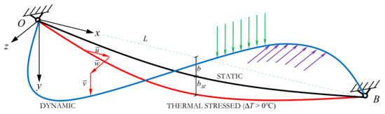
Figure 1.
Suspended cable’s mathematical model in thermal conditions.
The span of the cable between two horizontal supports, denoted by O and B, is measured as L. The original sag and thermal-stressed sag are represented by b and , respectively. Under the external excitation, the longitudinal, vertical, and out-of-plane displacements along three directions are expressed by , , and . The partial differential equations of motion in the in-plane and out-of-plane directions are derived using the classical condensed mathematical model [35,38,39].
where the suspended cable is subject to two external harmonic loads, and , with in-plane (out-of-plane) excitation amplitudes, frequencies, and phases represented by , , and , respectively. These loads apply a distributed force to the cable, with the cable’s Young’s modulus, cross-sectional area, and mass per length represented by E, A, and m, respectively. A notable deviation between the classical and original differential equations of motion governing the suspended cable and the current model is the introduction of a new tension variation factor [35]
where and are the cable tension force and sag with (without) thermal effects, respectively. Here, once the temperature changes are neglected , Equation (1) are reduced to the classical original partial differential equations in [10].
The following dimensionless variables and parameters are also defined
By substituting Equation (3) into (1) and removing the asterisk notations for simplicity, we obtain a set of dimensionless equations governing the in-plane and out-of-plane motions
where the eigenvalue solutions are derived by disregarding the non-linear, damping, and forcing terms (Appendix A).
To investigate internal resonances between in-plane and out-of-plane modes, we utilize two discretization equations
where denotes the n-th eigenfunction for the transverse (out-of-plane) motions. and represent the in-plane and out-of-plane generalized coordinates. By inserting Equation (5) into (4), integrating from 0 to 1, and multiplying by the mode shapes and , we obtain two ordinary differential equations
where details regarding the damping, excitation, linear, and non-linear coefficients can be found in Appendix B.
3. Perturbation Analysis and Modulation Equations
In line with the multiple scales procedure outlined in [45,46], we expand the unknown displacement coordinates and velocity coordinates as follows
where =, =, and =, .
By inserting Equation (7) and the time-derivative expansion into the governing equations and equating coefficients of equal powers of , we obtain the following six first-order differential equations of order , , and
Order
Order
Order
where and are the Kronecker delta functions.
One begins by obtaining solutions to the order equations, which can be derived as follows
where represents the conjugate for the preceding complex terms, and is the complex valued amplitude of the th mode.
Next, we substitute Equation (11) into the order equations and follow the same procedure outlined in [45] to obtain the corresponding second-order solutions
To quantify the proximity of external and internal resonances, we introduce two detuning parameters denoted by and .
where and are the in-plane and out-of-plane mode frequencies, respectively. is the excitation frequency which is applied on the in-plane or out-of-plane modes directly. and are the external and internal detuning parameters, respectively.
By substituting the previous second-order solutions into the order equations and introducing solvability conditions, we obtain the modulation equations governing and . Then, we employ the reconstitution method to express the modulation equations in the third-order
where the non-linear coefficients , , , , and are expressed in Appendix C.
Furthermore, and in Equation (14) can be written as in the polar forms , where and are the response amplitude and phase, respectively. Substituting the polar equations into Equation (14) and separating the real and imaginary parts, the polar form of modulation equations are obtained
where . , and , .
Similarly, the Cartesian form of modulation equations are also obtained
where . (the in-plane excitation), , and (the out-of-plane excitation), , .
The fixed points, also known as equilibrium or constant solutions, can be obtained by setting and in Equation (). Using a pseudo-arclength path-following algorithm, we trace the rest response branches and determine the corresponding stability of the fixed points based on the eigenvalues of the Jacobian matrix in Equation (16). Utilizing XPPAUTO, the four coupled solution branches that involve non-zero solutions and determines their stability properties are exhibited [47].
4. Numerical Examples and Illustrations
4.1. Parameters and Coefficients
The parameters adopted in the following numerical examples are shown in Table 1. Here, it is assumed that the density , cross-section area A, and material properties (Young’s modulus E and damping ratios ) are all independent of temperature variations. It is shown that the vibration characteristics are not sensitive to these temperature-dependent variables between −40 C and 40 C. In this following, it is noted that the temperature changes under consideration are not continuous values, but rather several deterministic values.

Table 1.
Parameters of the suspended cable.
The first two in-plane symmetric and the out-of-plane mode frequencies are plotted versus the corresponding Irvine parameter in Figure 2. It is known that the one-to-one internal resonance occurs for a specific set of system parameters, e.g., the closeness of two natural frequencies. Here, the first symmetric mode frequencies are equal to the second out-of-plane ones around the first crossover point. The natural frequencies of the system may undergo unexpected changes due to temperature variations. Due to the shift of natural frequencies, the crossover point is also shifted, so the one-to-one internal resonant case will be exhibited in different Irvine parameters since the temperature increases or decreases.
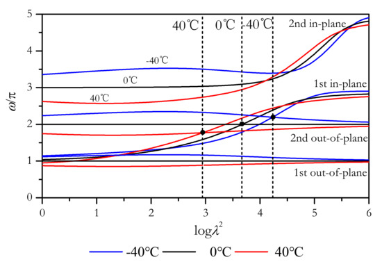
Figure 2.
The first two in-plane (symmetric) and out-of-plane mode frequencies of suspended cables in thermal environments.
In this work, we investigate internal resonances between the in-plane and out-of-plane modes, assuming that their natural frequencies are in close proximity to each other. The tension variation factor, natural frequencies, and the quadratic and cubic non-linear coefficients are given in Table 2. There are significant differences in these quadratic and cubic coefficients in warming and cooling conditions. Internal resonances in this classical quadratic and cubic non-linear system lead to strongly coupled motions, so the effective interaction coefficients with thermal effects around the first crossover point are also given in Table 3. Specifically, the tension force is decreased and the natural frequency is also decreased in the warming condition. The absolute values of all non-linear and effective interaction coefficients increase (decrease) when the temperature decreases (increases).
Table 2.
Linear and non-linear coefficients of in-plane and out-of-plane motions with thermal effects.
Table 3.
Effective interaction coefficients with thermal effects at the first crossover point (CP) between in-plane and out-of-plane mode shapes.
4.2. Bifurcation and Stability Analysis
This section presents numerical examples that investigate qualitative and quantitative changes and bifurcations in thermal environments. Force-response curves are obtained by selecting the external excitation amplitude as the control parameter, while frequency-response curves are obtained by adopting the detuning parameter as the control factor. The stable (unstable) solution branches are indicated by solid (dashed) lines, and the vibration behaviors in cooling and warming conditions are represented by blue and red lines (circles), respectively, using the perturbation (numerical) method.
4.2.1. In-Plane Excitations
Firstly, it is assumed that the external excitation is applied in the in-plane direction, and the force-response curves with thermal effects are discussed. Setting two detuning parameters and , the influences of the in-plane excitation amplitudes on the in-plane and out-of-plane responses in warming and cooling conditions are shown in Figure 3.
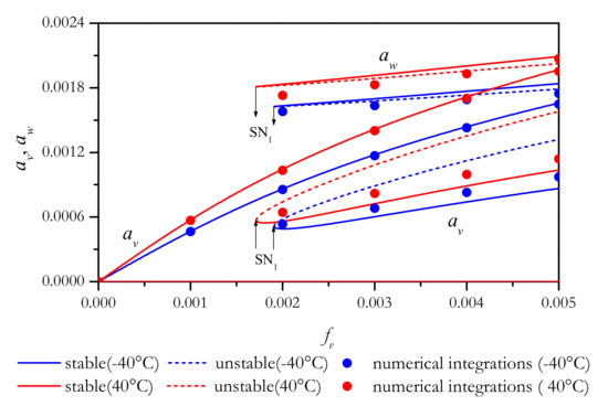
Figure 3.
Force-response amplitude curves with thermal effects when and .
As the excitation amplitude increases from zero, only a single-mode solution is exhibited and increases monotonously from 0 to . However, provided that the excitation amplitude is greater than approximately, another coupled branches appear for some selected initial conditions. As to these two-mode solutions, the non-planar coupled motions are exhibited, and the out-of-plane responses are greater than the in-plane ones. As the excitation amplitude decreases from , the steady-state responses decrease monotonously until the saddle-node bifurcation SN. It is known that SN is a typical static bifurcation and corresponds to the jump phenomenon, and the stability and number of periodic motion states are changed suddenly. As to these two types of solutions, two response amplitudes and in the warming condition are larger than the one in the cooling condition. The saddle-node bifurcation SN is exhibited at a smaller excitation amplitude in the warming condition.
Furthermore, some numerical integration solutions are presented by using the fourth-order Runge–Kutta method in Equation (6) directly. As shown in Figure 3, for the single-mode solutions, the perturbation ones are in excellent agreement with the numerical results. For the two-mode solutions, the numerical results seem a little larger than the perturbation ones as to the directly excited amplitudes . On the contrary, these numerical results seem a little smaller than the perturbation ones as to internally excited amplitudes . Although a little bit of difference is observed, the discrepancies induced by temperature effects are confirmed quantitatively by numerical simulations.
Figure 4 illustrates the force-response curves with thermal effects for the second group of detuning parameters, with and . Two types of solutions are presented: single-mode and two-mode and . For the single-mode solution, only in-plane motions are exhibited. As the excitation amplitude increases, the in-plane response also increases until reaching the first pitch-fork bifurcation PF. A jump phenomenon is observed, and the jump point comes earlier in the warming condition. Similarly, the response amplitude in the warming condition is larger than the one in the cooling condition. As to the coupled motions, when the forcing amplitude is dropped from , both the in-plane and out-of-plane response amplitudes are decreased accordingly until reaching the saddle-node bifurcation SN. Specifically, both the in-plane and out-of-plane response amplitudes decrease when the temperature drops from 40 C to −40 C. It is observed that the temperature effects on the saddle-node bifurcation are not apparent. Although there are some differences between the numerical solutions and perturbation ones in the coupled motions, the quantitative changes induced by thermal effects are confirmed.
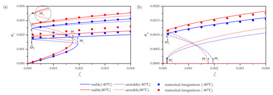
Figure 4.
Force-response amplitude curves with thermal effects when and : (a) in-plane; (b) out-of-plane.
For certain initial conditions, small excitation amplitudes can lead to extremely large vibration amplitudes due to internal resonances. These resonant responses are highly sensitive to temperature variations and resulting in energy transfer from in-plane to out-of-plane modes. Direct numerical simulations and perturbation methods demonstrate good agreement in this case, although some discrepancies are also observed.
Figure 5 presents typical frequency-response curves when and , exhibiting the temperature effects on the dynamic behaviors through bifurcation diagrams obtained using the external detuning parameter as a control factor. In the non-resonant region, numerical simulations yield a small steady-state solution, which is used as the starting point for a pseudo-arclength continuation to construct the rest curves. As the excitation detuning parameter decreases from , only in-plane motions are observed in the small response region, with out-of-plane motions remaining at zero. The frequency-response curves bend to the left side, indicating a softening-type response of the non-linear system. Notably, as the temperature drops from 40 C to −40 C, the curves show an even greater leftward bend.
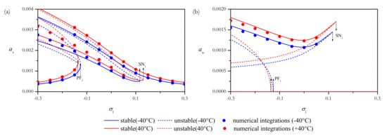
Figure 5.
Frequency-response amplitude curves with thermal effects when and : (a) in-plane; (b) out-of-plane.
Two types of bifurcations, saddle-node bifurcation SN and pitch-fork bifurcation PF, are observed in the force-response curves, with the pitch-fork bifurcation occurring at a smaller detuning parameter in the warming condition and the saddle-node bifurcation occurring at a larger detuning parameter in the same condition. As a result, the resonant region between the two bifurcations becomes larger at higher temperatures. These internal resonant phenomena can easily be excited under very small external excitation amplitudes and become more sensitive to temperature variations. From a non-linear dynamics perspective, these observations highlight the importance of considering internal resonances and their sensitivity to temperature in the study of vibrational behavior.
Exciting a non-linear system near Hopf bifurcations can cause the system’s natural frequencies to change due to thermal effects, resulting in sudden and significant changes in response amplitude. From a non-linear dynamics perspective, this phenomenon is due to the coupling between non-linear behavior and thermal effects, highlighting the importance of considering temperature effects in the study of non-linear vibrations. For this reason, to clarify the temperature effects further, the time histories, phase planes, Poincare sections, and power spectra are presented to exhibit the dynamic responses on the non-linear system in thermal environments for some selected parameters (, , and , , ), just as shown in Figure 6 and Figure 7.
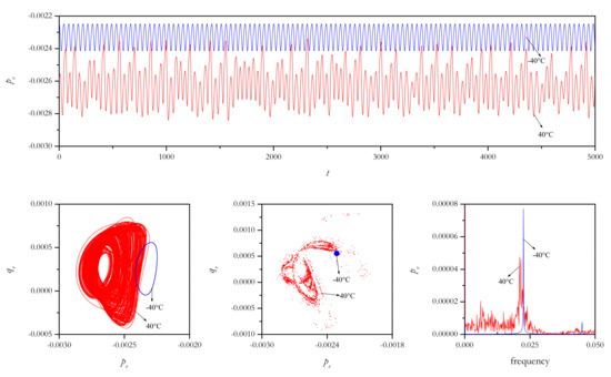
Figure 6.
Time history curves, phase plane portraits, Poincaré sections and FFTs with thermal effects when , , and .
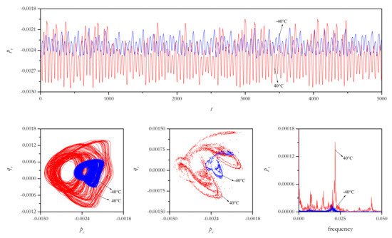
Figure 7.
Time history curves, phase plane portraits, Poincaré sections and FFTs with thermal effects when , , and .
Some essential differences induced by temperature changes are observed. As shown in Figure 6, the suspended cable exhibits periodic motion in the cooling condition. A single circle is observed in the phase plane portrait, a single dot is noted in the Poincaré section, and a main frequency could be observed in the frequency spectrum. In the warming condition, the previous periodic motion bifurcated into chaotic motions. The time history curves presented in Figure 6 indicate that the system’s response is chaotic, a conclusion supported by the corresponding phase plane, frequency spectra, and Poincar’e sections. From a non-linear dynamics perspective, it can be observed that periodic motions bifurcate into chaotic ones as the temperature increases from −40 C to 40 C, emphasizing the significant impact of temperature on the system’s non-linear behavior. Dynamic chaos and oscillations are an essential undesired non-linear phenomena in cable structures, and they may induce undesired destructions of the discomfort of the non-linear system. Here, the temperature changes become the key factor, and the chaos may be excited in different temperature conditions.
Figure 7 illustrates that the non-linear system exhibits chaotic motions in both warming and cooling conditions, with similarities observed in their phase plane diagrams and chaotic attractors. However, a significant difference is observed in the response amplitudes, which are reduced in the warming condition. These observations highlight the sensitivity of chaotic motions to temperature changes from a non-linear dynamics perspective.
4.2.2. Out-of-Plane Excitations
Provided that the external excitation is transferred from the in-plane to the out-of-plane, the relative dynamical behaviors are investigated. Figure 8 presents the force-response curves when and , and the out-of-plane excitation amplitude is selected as the control parameter. As shown in Figure 8, there is no stable equilibrium solution in the middle of the resonant region. In this region, the suspended cable’s responses are expected to be either periodic or chaotic modulation motions.
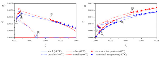
Figure 8.
Force-response amplitude curves with thermal effects when and : (a) in-plane; (b) out-of-plane.
If the out-of-plane excitation amplitude increases from zero, only the out-of-plane motions could be observed. The steady-state solutions are stable until reaching the pitch-fork bifurcation PF. If increases further, the branch gains stability again at the Hopf bifurcation HB, where the response branches as to the in-plane motion emerge. Along these branches, there is strong coupling between the in-plane and out-of-plane motions. As to some small excitation amplitudes, there are some large response amplitudes due to the one-to-one internal resonances. It is noticed that there are two saddle nodes, and the non-linear internal resonant responses are stable between these two bifurcations while it is unstable in other regions. Within the internal resonant region, the internal excited amplitudes appear to be more sensitive to temperature changes than the directly excited ones .
Otherwise, when sweeping the out-of-plane excitation amplitude backward from , the out-of-plane (in-plane) response amplitude () decreases (increases) and passes through a Hopf bifurcation in the internal resonant region. Then, a stable solution starts to fade away and passes through a pitch-fork bifurcation. As illustrated before, the response amplitude decreases (increases) in the cooling (warming) condition, regardless of the direct or the internal resonant case. Interestingly, in the large excitation amplitude region (e.g., ), the internal excitation amplitude decreases (increases) in the warming (cooling) condition on the contrary. Both the perturbations and numerical solutions have verified this phenomenon. Here, both the static and dynamic bifurcations could be observed. Due to the temperature effects, three bifurcations (PF, SN, and HB) are exhibited in a smaller excitation amplitude in the warming condition.
Finally, Figure 9 illustrates the representative frequency response curves when the external excitation is applied on the out-of-plane direction. The corresponding bifurcations are marked, and the stability of the steady-state solutions is described clearly. These curves show the response amplitudes and as a function of the external detuning parameter , for fixed values of the out-of-plane excitation amplitude and the internal detuning parameter .
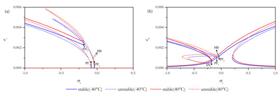
Figure 9.
Frequency-response amplitude curves with thermal effects when and : (a) in-plane; (b) out-of-plane.
Specifically, Figure 9 reveals that for , only the single-mode solution is observed, and the in-plane response amplitude remains at zero. However, for , a strong interaction between the in-plane and out-of-plane modes is expected, and an internal resonance may occur, leading to a sudden appearance in the response amplitude of the in-plane mode due to energy transfer from the out-of-plane mode. In the internal resonant region, further sweeping of the external detuning parameter causes a decrease in the in-plane and out-of-plane responses until they experience a saddle-node jump to the trivial solutions. It is observed that increasing temperature significantly reduces the response amplitudes. In this case, three bifurcations are observed to be excited at a smaller detuning parameter in the warming condition, emphasizing the importance of considering temperature effects on the system’s non-linear behavior from a non-linear dynamics perspective.
5. Conclusions
In thermal environments, suspended cables experience unexpected changes in their natural frequencies and mode shapes, resulting in shifted crossover points between in-plane and out-of-plane mode frequencies. Non-linear and effective interaction coefficients also increase or decrease with changes in temperature. When external excitation is applied in the in-plane direction, decreasing temperature leads to significant changes in resonant responses by reducing response amplitudes. However, when external force is applied in the out-of-plane direction, the out-of-plane response amplitude decreases with decreasing temperature, while the in-plane response amplitude increases with decreasing temperature at large excitation amplitudes. Additionally, smaller excitation amplitudes and frequencies can excite the saddle-node, pitch-fork, and Hopf bifurcations when the temperature increases, and periodic motions may transition to chaotic ones. Perturbation and numerical solutions agree well in the non-internal resonant region, but the perturbation solutions slightly overestimate or underestimate the response amplitude in direct or internal excited modes when the one-to-one internal resonance is excited.
Author Contributions
Conceptualization, W.N. and Y.Z.; methodology, Z.G.and H.L.; software, Z.G. and H.L.; validation, Z.G. and H.L.; formal analysis, Z.G. and H.L.; investigation, Z.G. and H.L.; writing—original draft preparation, Z.G., H.L. and Y.Z.; writing—review and editing, H.L., W.N. and Y.Z.; visualization, W.N. and Y.Z.; supervision, W.N. and Y.Z.; funding acquisition, W.N. and Y.Z. All authors have read and agreed to the published version of the manuscript.
Funding
The research described in this paper was financially supported by National Natural Science Foundation of China (No. 12272139), Natural Science Foundation of Fujian Province (No. 2022J01290) and Collaborative Innovation Platform Project of Fuzhou-Xiamen-Quanzhou National Self-Innovation Zone (3502ZCQXT2022002).
Institutional Review Board Statement
Not applicable.
Informed Consent Statement
Not applicable.
Data Availability Statement
The relevant data are all included in the paper.
Conflicts of Interest
The authors declare no conflict of interest in preparing this article.
Appendix A
By solving the transcendental equations, we obtain the in-plane symmetric mode frequencies
where
and the in-plane symmetric mode shapes are expressed as
where the coefficient is ascertained through .
As to in-plane anti-symmetric and out-of-plane mode shapes and frequencies are expressed as follows
where all these natural frequencies are dependent on the temperature changes and these mode shapes are independent of temperature conditions.
Appendix B
Appendix C
References
- Warminski, J.; Zulli, D. Revisited modelling and multimodal non-linear oscillations of a sagged cable under support motion. Meccanica 2016, 51, 2541–2575. [Google Scholar] [CrossRef]
- Yi, Z. Stanciulescu I. Non-linear normal modes of a shallow arch with elastic constraints for two-to-one internal resonances. Non-Linear Dyn. 2016, 83, 1577–1600. [Google Scholar] [CrossRef]
- Qiao, W.; Guo, T.; Kang, H.; Zhao, Y. An asymptotic study of non-linear coupled vibration of arch-foundation structural system. Eur. J. Mech. Solid. 2022, 96, 104711. [Google Scholar] [CrossRef]
- Peng, J.; Xiang, M.; Wang, L.; Xie, X.; Sun, H.; Yu, J. Non-linear primary resonance in vibration control of cable-stayed beam with time delay feedback. Mech. Sys. Sig. Proc. 2020, 137, 106488. [Google Scholar] [CrossRef]
- Cong, Y.; Kang, H.; Yan, G.; Guo, T. Modeling, dynamics, and parametric studies of a multi-cable-stayed beam model. Acta Mech. 2020, 231, 4947–4970. [Google Scholar] [CrossRef]
- Gattulli, V.; Lepidi, M.; Potenza, F.; Sabatino, U.D. Modal interactions in the non-linear dynamics of a beam-cable-beam. Non-Linear Dyn. 2019, 96, 2547–2566. [Google Scholar] [CrossRef]
- Sun, C.; Jiao, D.; Lin, J.; Li, C.; Tan, C. Modal characteristics of sagged-cable-crosstie systems. Part 1: Modeling and validation. Appl. Math. Model. 2023, 119, 698–716. [Google Scholar] [CrossRef]
- Sun, C.; Liu, W.; Jiao, D.; Li, C. Modal characteristics of sagged-cable-crosstie systems. Part 2: Parametric analysis. Appl. Math. Model. 2023, 119, 549–565. [Google Scholar] [CrossRef]
- Wang, Z.; Li, T.; Yao, S. Non-linear dynamic analysis of space cable net structures with one to one internal resonances. Non-Linear Dyn. 2014, 78, 1461–1475. [Google Scholar] [CrossRef]
- Rega, G. Non-linear vibrations of suspended cables Part I: Modeling and analysis. Appl. Mech. Rev. 2004, 57, 443–478. [Google Scholar] [CrossRef]
- Srinil, N.; Rega, G.; Chucheepsakul, S. Large amplitude three-dimensional free vibrations of inclined sagged elastic cables. Non-Linear Dyn. 2003, 33, 129–154. [Google Scholar] [CrossRef]
- Rega, G. Non-linear vibrations of suspended cables, Part II: Deterministic phenomena. Appl. Mech. Rev. 2004, 57, 479–514. [Google Scholar] [CrossRef]
- Perkins, N.C. Modal interactions in the non-linear response of elastic cables under parametric/external excitation. Int. J. Non-Linear Mech. 1992, 27, 233–250. [Google Scholar] [CrossRef]
- Benedettini, F.; Rega, G.; Alaggio, R. Non-linear oscillations of a four-degree-of-freedom model of a suspended cable under multiple internal resonance conditions. J. Sound Vib. 1995, 182, 775–798. [Google Scholar] [CrossRef]
- Pakdemirli, M.; Nayfeh, S.A.; Nayfeh, A.H. Analysis of one-to-one autoparametric resonances in cables—Discretization vs. direct treatment. Non-Linear Dyn. 1995, 8, 65–83. [Google Scholar] [CrossRef]
- Lee, C.; Perkins, N.C. Three-dimensional oscillations of suspended cables involving simultaneous internal resonances. Non-Linear Dyn. 1995, 8, 45–63. [Google Scholar] [CrossRef]
- Rega, G.; Lacarbonara, W.; Nayfeh, A.H.; Chin, C.M. Multiple resonances in suspended cables: Direct versus reduced-order models. Int. J. Non-Linear Mech. 1999, 34, 901–924. [Google Scholar] [CrossRef]
- Nayfeh, A.H.; Chin, C.M.; Lacarbonara, W. Multimode interactions in suspended cables. J. Vib. Control 2002, 8, 337–387. [Google Scholar] [CrossRef]
- Gattulli, V.; Martinelli, L.; Perotti, F.; Vestroni, F. Non-linear oscillations of cables under harmonic loading using analytical and finite element models. Comput. Methods Appl. Mech. Eng. 2004, 193, 69–85. [Google Scholar] [CrossRef]
- Berlioz, A.; Lamarque, C.-H. A non-linear model for the dynamics of an inclined cable. J. Sound Vib. 2005, 279, 619–639. [Google Scholar] [CrossRef]
- Srinil, N.; Rega, G. The effects of kinematic condensation on internally resonant forced vibrations of shallow horizontal cables. Int. J. Non-Linear Mech. 2007, 42, 180–195. [Google Scholar] [CrossRef]
- Gonzalez-Buelga, A.; Neild, S.A.; Wagg, D.J.; Macdonald, J.H.G. Modal stability of inclined cables subjected to vertical support excitation. J. Sound Vib. 2008, 318, 565–579. [Google Scholar] [CrossRef]
- Abe, A. Validity and accuracy of solutions for non-linear vibration analyses of suspended cables with one-to-one internal resonance. Non-Linear Anal. Real World Appl. 2010, 11, 2594–2602. [Google Scholar] [CrossRef]
- Luongo, A.; Zulli, D. Dynamic instability of inclined cables under combined wind flow and support motion. Non-Linear Dyn. 2012, 67, 71–87. [Google Scholar] [CrossRef]
- Guo, T.; Kang, H.; Wang, L.; Zhao, Y. Cable’s non-planar coupled vibrations under asynchronous out-of-plane support motions: Travelling wave effect. Arch. Appl. Mech. 2016, 86, 1647–1663. [Google Scholar] [CrossRef]
- Macdonald, J.H.G. Multi-modal vibration amplitudes of taut inclined cables due to direct and/or parametric excitation. J. Sound Vib. 2016, 363, 473–494. [Google Scholar] [CrossRef]
- Zulli, D.; Piccardo, G.; Luongo, A. On the non-linear effects of the mean wind force on the galloping onset in shallow cables. Non-Linear Dyn. 2021, 103, 3127–3148. [Google Scholar] [CrossRef]
- Nayfeh, A.H. Non-linear Interactions: Analytical, Computational, and Experimental Method; Wiley Series in Non-linear Science; Wiley: New York, NY, USA, 2000. [Google Scholar]
- Manevich, A.I.; Manevich, L.I. The Mechanics of Non-linear Systems with Internal Resonances; Imperial College Press: London, UK, 2005. [Google Scholar]
- Xia, Y.; Chen, B.; Weng, S.; Ni, Y.Q.; Xu, Y.L. Temperature effect on the vibration properties of civil structures: A literature review and case studies. J. Civ. Struct. Health Monit. 2012, 2, 29–46. [Google Scholar] [CrossRef]
- Treyssède, F. Finite element modeling of temperature load effects on the vibration of local modes in multi-cable structures. J. Sound Vib. 2018, 413, 191–204. [Google Scholar] [CrossRef]
- Zhou, H.; Ni, Y.Q.; Ko, J.M. Eliminating temperature effect in vibration-based structural damage detection. J. Eng. Mech. 2011, 137, 785–796. [Google Scholar] [CrossRef]
- Ma, L.; Xu, H.; Munkhbaatar, T.; Li, S. An accurate frequency-based method for identifying cable tension while considering environmental temperature variation. J. Sound Vib. 2021, 490, 115693. [Google Scholar] [CrossRef]
- Montassar, S.; Mekki, O.B.; Vairo, G. On the effects of uniform temperature variations on stay cables. J. Civ. Struct. Health Monit. 2015, 5, 735–742. [Google Scholar] [CrossRef]
- Lepidi, M.; Gattulli, V. Static and dynamic response of elastic suspended cables with thermal effects. Int. J. Solids Struct. 2012, 49, 1103–1116. [Google Scholar] [CrossRef]
- Bouaanani, N.; Marcuzzi, P. Finite difference thermoelastic analysis of suspended cables including extensibility and large sag effects. J. Therm. Stress. 2011, 34, 18–50. [Google Scholar] [CrossRef]
- Treyssède, F. Free linear vibrations of cables under thermal stress. J. Sound Vib. 2009, 327, 1–8. [Google Scholar] [CrossRef][Green Version]
- Zhao, Y.; Peng, J.; Zhao, Y.; Chen, L. Effects of temperature variations on non-linear planar free and forced oscillations at primary resonances of suspended cables. Non-Linear Dyn. 2017, 89, 2815–2827. [Google Scholar] [CrossRef]
- Zhao, Y.; Huang, C.; Chen, L.; Peng, J. Non-linear vibration behaviors of suspended cables under two-frequency excitation with temperature effects. J. Sound Vib. 2018, 416, 279–294. [Google Scholar] [CrossRef]
- Zhao, Y.; Huang, C.; Chen, L. Non-linear planar secondary resonance analyses of suspended cables with thermal effects. J. Therm. Stress. 2019, 42, 1515–1534. [Google Scholar] [CrossRef]
- Zhao, Y.; Zheng, P. Parameter analyses of suspended cables subjected to simultaneous combination, super and sub-harmonic excitations. Steel Compos. Struct. 2021, 40, 203–216. [Google Scholar]
- Zheng, P.; Zhao, Y.; Wu, X.; Chen, L. Revisited modeling and non-linear oscillation behaviors of multi-segment damaged suspended cables in thermal environments. Meccanica 2022, 57, 1831–1851. [Google Scholar] [CrossRef]
- Zhao, Y.; Zheng, P.; Lin, H.; Chen, L. Non-linear coupled dynamics of suspended cables due to crossover points shifting and symmetry breaking. Eur. J. Mech. A-Solid. 2023, 99, 104921. [Google Scholar] [CrossRef]
- Zhao, Y.; Lin, H. Non-linear dynamics of suspended cables in thermal environments under periodic excitation: Two-to-one internal resonance. Int. J. Bifurcat. Chaos. 2021, 31, 2150153. [Google Scholar] [CrossRef]
- Lacarbonara, W.; Rega, G.; Nayfeh, A.H. Resonant nonliear normal modes. Part I: Analytical treatment for structural one-dimensional systems. Int. J. Non-Linear Mech. 2003, 38, 851–872. [Google Scholar] [CrossRef]
- Lacarbonara, W.; Rega, G. Resonant nonliear normal modes. Part II: Activation/orthogonality conditions for shallow structural systems. Int. J. Non-Linear Mech. 2003, 38, 873–887. [Google Scholar] [CrossRef]
- Ermentrout, B. Simulating, Analyzing, and Animating Dynamical Systems: A Guide to XPPAUT fro Researchers and Students; SIAM: Philadelphia, PA, USA, 2002. [Google Scholar]


Disclaimer/Publisher’s Note: The statements, opinions and data contained in all publications are solely those of the individual author(s) and contributor(s) and not of MDPI and/or the editor(s). MDPI and/or the editor(s) disclaim responsibility for any injury to people or property resulting from any ideas, methods, instructions or products referred to in the content. |
© 2023 by the authors. Licensee MDPI, Basel, Switzerland. This article is an open access article distributed under the terms and conditions of the Creative Commons Attribution (CC BY) license (https://creativecommons.org/licenses/by/4.0/).