Arbitrary-Order Sensitivity Analysis of Eigenfrequency Problems with Hypercomplex Automatic Differentiation (HYPAD)

Featured Application

Sensitivity analysis of the modal response in structural systems.

Abstract

The calculation of accurate arbitrary-order sensitivities of eigenvalues and eigenvectors is crucial for structural analysis applications, including topology optimization, system identification, finite element model updating, damage detection, and fault diagnosis. Current approaches to obtaining sensitivities for eigenvalues and eigenvectors lack generality, are complicated to implement, prone to numerical errors, and are computationally expensive. In this work, a novel methodology is introduced that uses hypercomplex automatic differentiation (HYPAD) and semi-analytical expressions to obtain arbitrary-order sensitivities for eigenfrequency problems. The new methodology exhibits no sign of truncation nor subtractive cancellation errors regardless of the order of the sensitivity, it is general, and can obtain any high-order sensitivities with the simplicity of first-order computations. A numerical example is presented to verify the accuracy of the method, where the free vibration of a homogeneous cantilever beam is studied. For this problem, up to third-order sensitivities of the eigenvalues and eigenvectors with respect to the material and geometrical parameters were obtained, considering the cases of close and distinct eigenvalues. The results were verified using analytical equations, showing excellent agreement for the eigenvalues and the eigenvectors. The new method promises to facilitate the computation of sensitivities for eigenfrequency problems into routine practice and commercial software.

1. Introduction

In structural design and analysis, it is crucial to obtain the natural frequencies (eigenvalues) and mode shapes (eigenvectors) of structures because they provide insights into the systems’ dynamical characteristics. These characteristics are assessed by solving the eigenfrequency problem and are highly affected by changes in the mechanical properties of the materials forming the structure, the external loads, and the geometry of the models. Hence, calculating the sensitivities of the eigenvalues and eigenvectors with respect to the input parameters of the model has been considered an important research topic since the early 1960s [1]. In addition to understanding how the structures are affected by changes in the models’ input variables [2], the sensitivity analysis of eigenvalues and eigenvectors is used in optimization design [3], damage detection and fault diagnosis [4], finite element model updating [5], topology optimization [6], uncertainty quantification [7], and system identification [5]. For these applications, most of the current methods used to obtain sensitivities for the eigenvalues and eigenvectors are restricted to first-order approximations. Although first-order approximations are adequate for most cases, when dealing with complex systems the magnitude of the modelling errors becomes substantial, leading to numerical issues. These issues can produce slow convergence rates of optimization or updating algorithms [4], or even divergence (i.e., no optimal result is reached). Therefore, higher-order sensitivities are needed to further improve the numerical accuracy and performance.

The eigenvalues and eigenvectors of large complex structures are obtained by solving the generalized eigenvalue problem (GEP). In the GEP, the system’s equation of motion is solved in the frequency domain, assuming a time-harmonic solution and a zero-loading condition. For the GEP, the eigenvalues and eigenvectors are calculated in different steps. For most structures, closed form solutions of the eigenvalues do not exist; therefore, these are found by using numerical methods, such as the QR method [8,9], Implicit Lanczos iteration [10], and the Davidson Method [11], among others. The eigenvectors are obtained algebraically by replacing the eigenvalues’ numerical results into the equation of motion. As the GEP is solved numerically, this represents a major challenge when calculating higher-order sensitivities in eigenfrequency problems. Different methods have been proposed to calculate the sensitivities for the eigenvalues and eigenvectors. Because these two are calculated in different steps, the methodologies have been developed independently from each other.

For obtaining the sensitivities of the eigenvalues, most of the work available in the literature is focused on implementing iterative schemes and developing semi-analytical expressions derived from the governing equation of the GEP [12,13,14,15]. Iterative methods are only efficient for systems with limited design variables as iterations are required for each independent variable; thus, these methods become computationally expensive specially in systems with a large number of degrees of freedom (DOF). In the case of semi-analytical methods [16,17,18,19,20,21], the eigenvalues, eigenvectors, and the sensitivities of the stiffness $[K$] and mass $\left[M\right]$ matrices are plugged into the semi-analytical expressions to calculate the sensitivities of the eigenvalues. The work by Fox and Kapoor [17] is considered seminal in this area. Although the method proposed by these authors is limited to first-order sensitivities, the expression to obtain the eigenvalue sensitivities can be expanded to higher-order sensitivities with minimal additional effort; however, the equations become lengthy and complicated to implement.

Approximate numerical differentiation methods have also been used to calculate eigenvalue sensitivities, including finite differentiation methods (FD) and complex variable methods (CVM). The FD computes derivatives by adding a real-valued perturbation to the objective function, in this case, the GEP equation. Computing an FD approximation of a derivative is straightforward. However, the difficulties are given by the step size dependency, computational cost, and subtraction errors inherent to the method [22,23,24]. In contrast, CVM uses complex variables to compute the sensitivities of eigenvalues. Wang and Apte [25] presented an accurate, robust, and easy-to-implement CVM to differentiate eigenvalues. This method is only available for first-order sensitivities, and it requires numerical solvers for the GEP capable of handling complex algebra. Furthermore, Navarro et al. [26] presented a CVM to compute arbitrary-order eigenvalue sensitivities in Phononic Materials using the QR decomposition method; however, the method becomes impractical for a large number of sensitivities in systems with a high number of DOF because it requires several iterations over large matrices. In addition, it calculates the derivatives for all the eigenvalues corresponding to all the DOF in the system without distinction, increasing the computational complexity. Recently, Fujikawa et al. [27] introduced a CVM to differentiate eigenvalues and eigenvectors using hyperdual numbers. Although arbitrary-order sensitivities can be computed with such approach, the method involves the solution of multiple linear systems of equations for computing the sensitivities of both the eigenvalues and eigenvectors, which increases the computational cost. In addition, the method has problems when calculating the sensitivities of systems that exhibit repeated eigenvalues.

The calculation of the sensitivities of the eigenvectors for systems with repeated eigenvalues has been reported as a challenging and open area of research [6]. A model with distinct eigenvalues has one unique eigenvector for each eigenvalue. This implies that the eigenvectors are orthonormal and continuously differentiable with respect to any model input parameters. In contrast, a model with repeated or close eigenvalues has many orthonormal eigenvectors associated with multiple eigenvalues. This adversely affects the differentiability and continuity of the eigenvectors with respect to the model input parameters [6]. In the literature, there are two commonly used methods for calculating sensitivities of eigenvectors: model superposition methods [17,28] and Nelson-like methods [29]. These methods use semi-analytical expressions and work when repeated and distinct eigenvalues are available. The modal superposition methods calculate the sensitivities of the eigenvectors with a linear superposition of all the structure’s eigenvalues and eigenvectors. As obtaining all the modes in large systems is computationally expensive, these methods become impractical. Nonetheless, improvements have been proposed where the eigenvector sensitivities can be approximated using only a smaller set of modes [30,31,32]. As the superposition is truncated with these modifications the computations become prone to numerical errors.

In addition, the modal superposition methods are complicated to implement because of the complexity of the semi-analytical equations, especially for higher-order sensitivities [33]. Nelson-like methods were originally presented in [29], with the main advantage of requiring only the information from the modes of interest to compute the sensitivities of the eigenvectors in distinct eigenvalues problems. Several authors [34,35,36,37] made extensions to the initial approach, including the capabilities to deal with repeated eigenvalues [38,39], and to expand the method to obtain higher-order sensitivities [21,40]. Although these methods are efficient, the implementation of the algorithms tends to be cumbersome because the semi-analytical equations used to obtain the sensitivities change depending on the position of the largest magnitude component of each eigenvector being differentiated. In some cases, these changes result in the solution of ill-conditioned systems of equations [30]. Yang et al. [33] addressed these problems by introducing a general semi-analytical expression to obtain sensitivities that are independent of the characteristics of the eigenvectors. In this approach, only the eigenvalues and eigenvectors of the modes of interest, and the sensitivities for $[M$] and $\left[K\right]$ are needed to calculate the eigenvector sensitivities. This methodology is available for first and second-order derivatives and has been demonstrated in test cases that exhibit distinct and repeated eigenvalues. However, although the semi-analytical expression can be expanded to arbitrary-order, it becomes lengthy, making it difficult to implement within commercial software. In addition, obtaining the sensitivities for $\left[M\right]$ and $\left[K\right]$ is not trivial and it is prone to error, especially when estimating higher-order sensitivities [41].

The sensitivities for $\left[M\right]$ and $\left[K\right]$ are calculated either analytically [35,42], or by using first-order FD approximations [43]. The analytical approach is limited because $\left[K\right]$ and $\left[M\right]$ are typically estimated numerically. On the other hand, FD presents the same inaccuracy and step size dependency problems highlighted before [44]. Several attempts have been made to develop alternative methodologies to improve the accuracy of the numerical differentiation of the system matrices using FD. For instance, in the works by Olhoff et al. [45,46], a machine precision method for numerical differentiation of system matrices was presented. In this method, the first-order forward difference expression was corrected by using a set of scalar and matrix functions. In addition, in Bletzinger et al. [47], correction factors related to the rigid body rotations of the specific finite element formulations were introduced to the FD to calculate machine precision sensitivities. Despite these efforts, the methods are limited to finite element formulations based on Hermite Shape functions and only work for first-order approximations of the sensitivities.

As noted in our review, the calculation of higher-order sensitivities in eigenfrequency problems is limited by several technical issues. These include the unavailability of expressions to calculate higher-order sensitivities of the eigenvalues and eigenvectors that are general, computationally efficient, and easy-to-implement; and the absence of a general method to compute high-order derivatives for $[K$] and $\left[M\right]$. These facts have limited the widespread implementation of the current methods into computational practice and commercial software. In this work, these technical challenges are addressed by introducing a novel methodology to obtain arbitrary-order sensitivities for undamped eigenfrequency problems that takes advantage of the hypercomplex automatic differentiation (HYPAD) method. Recently, Lantoine et al. introduced HYPAD to obtain arbitrary-order sensitivities without truncation errors [48] using multicomplex algebra. HYPAD consists of multiple non-parallel independent imaginary axes used to perform function evaluations. The calculation of high-order and mixed partial sensitivities is obtained by perturbing the parameter of interest along the various imaginary axes, evaluating the function of interest, and extracting the imaginary components of the solution. Furthermore, when the subset of hypercomplex numbers, known as multidual as opposed to multicomplex, are used in HYPAD, no truncation and subtraction cancellation errors are produced in computing the derivatives [49]. Since its inception, HYPAD has been verified in several engineering applications, such as linear elastic analysis [50], fatigue [51,52], thermoelasticity [53,54], fracture mechanics [55,56,57], plasticity [58], viscoelasticity[59], residual stresses [60], creep [61], heat transfer [62], variance estimates [63], localization analysis [64] and system reliability analysis [65], among others.

In this work, we introduce a novel differentiation method for eigenvalues and eigenvectors that employs a single expression to accurately compute the machine precision sensitivities, regardless of the order of derivatives involved. This approach stands in contrast to existing methods, which often prove cumbersome to implement, particularly when dealing with higher-order sensitivities. By introducing this novel approach, we aim to simplify the implementation process and overcome the challenges associated with computing higher-order sensitivities in eigenvalue problems. Here, HYPAD is formulated within a discrete continuum approach based on the Finite Element Method (FEM) to obtain highly accurate arbitrary-order sensitivities of the mass and stiffness matrices with respect to any input parameter. Then, this sensitivity information is linked with the expressions to calculate the sensitivities of eigenvalues and eigenvectors presented by Fox and Kapoor [17] and Yang et al. [33], which are also numerically differentiated using HYPAD. It should be noted that although the method is presented using the FEM, it can be implemented using any discretization and spatial integration, such as the Boundary Element Method (BEM), isogeometric analysis (IGA) or the Spectral Finite Element Method (SFEM). The outline of the paper is as follows: Section 2 provides background information, including the expressions for the calculation of sensitivities in eigenfrequency problems derived by Fox and Kapoor [17] and Yang et al. [33], and a brief introduction to HYPAD. Section 3 introduces the new methodology to calculate arbitrary-order sensitivities of the eigenvalues and eigenvectors on eigenfrequency problems using HYPAD. Section 4 provides an analytical and numerical verification example of the new methodology used to compute eigenvalue and eigenvector sensitivities using HYPAD. The analytical example corresponds to a simple harmonic oscillator, and the numerical example corresponds to the free vibration of a rectangular cross-section cantilevered beam. Section 5 discusses the key issues of the methodology and expansions to other fields. Finally, in Section 6, conclusions and future work are presented.

2. Background

2.1. First Order Sensitivities of Eigenvalues and Eigenvectors

In this section, the methodologies derived by Fox and Kapoor [17] to calculate eigenvalues’ sensitivities, and from Yang and Peng [33] for eigenvectors’ sensitivities are reviewed. Consider the equation of motion in the frequency domain for a linear undamped discrete system subjected to harmonic loading:

$$\begin{array}{c}\left[F_i\right]{\varphi }_i=\left[K-{\lambda }_{i}M\right]{\varphi }_i=0\end{array}$$

(1)

Equation (1) corresponds to the Generalized Eigenvalue Problem (GEP), where $\left[F_i\right]=\left[K-{\lambda }_{i}M\right]$, ${\lambda }_i$ and ${\varphi }_i$ are the $i^{th}$ eigenvalue and right eigenvectors, respectively, $i=1,2,\dots ,n$ corresponds to the identifier of the $i^{th}$ mode of vibration, and $n$ identifies the number of DOF in the system. In structural problems, $\left[M\right]$ and $\left[K\right]$ correspond to $n\times n$ self-adjoint matrices representing the mass and stiffness, respectively. These matrices are symmetric, and their components are functions of the $j$ number of input parameters of the model, $\mathit{\alpha }=\{{\alpha }_1,\dots ,{\alpha }_j\}$, such as elastic modulus, geometry, and density. Depending on the geometrical characteristics of the system, Equation (1) can produce repeated or distinct eigenvalues. In the first case, there is a unique eigenvector ${\varphi }_i$ for each eigenvalue ${\lambda }_i$, and in the second case, each eigenvalue can have two or more eigenvectors associated (e.g., systems with geometrical symmetries) [35].

Equation (1) has a non-trivial solution for the orthogonal eigenvectors ${\varphi }_i$; therefore, these can be scaled by any magnitude and still be a basis of the system. For this reason, normalization is required to guarantee uniqueness in the solution [66]. In this work, mass normalization is used for all eigenvectors, satisfying ${\varphi }_i^T\left[M\right]{\varphi }_i=1$. This specific type of normalization is required to make the expressions presented below valid.

Taking the GEP defined in Equation (1), and premultiplying by ${\varphi }_i$, gives:

$$\begin{array}{c}{\varphi }_i^T\left[F_i\right]{\varphi }_i=0\end{array}$$

(2)

Equation (2) is differentiated to calculate the sensitivity of the eigenvalues with respect to any input parameter of the model ${\alpha }_j$. By making use of the conditions of the orthogonality of the eigenvectors and the mass normalization, the first-order derivative of the $i^{th}$ eigenvalue is calculated as:

$$\begin{array}{c}\frac{\partial {\lambda }_i}{\partial \alpha }={\varphi }_i^T\left[\frac{\partial K}{\partial \alpha }-{\lambda }_i\frac{\partial M}{\partial \alpha }\right]{\varphi }_i\end{array}$$

(3)

where Equation (3) corresponds to the exact solution for the first-order sensitivities of eigenvalues in structural systems as previously reported by Fox and Kapoor [17]. Note that this equation requires knowledge of the sensitivities of the stiffness and the mass matrices, $\left[\partial K/\partial \alpha \right]$ and $[\partial M/\partial \alpha ]$.

In the case of eigenvectors’ sensitivities, Yang and Peng derived exact expressions for the first- and second-order derivatives for distinct and repeated eigenvalues [33]. The first-order derivative of the $i^{th}$ eigenvector with respect to a design parameter ${\alpha }_j$ is:

$$\begin{array}{c}\frac{\partial {\varphi }_i}{\partial \alpha }=\left[{{\mathsf{\Theta }}_i]}^{-1}\right[{\mathsf{\Pi }}_i]{\varphi }_i\end{array}$$

(4)

where

$$\left[{\mathsf{\Theta }}_i\right]=\left[K\right]-{\lambda }_i\left[M\right]+{\lambda }_i{\varphi }_i{\varphi }_i^T\left[M\right]$$

$$\left[{\mathsf{\Pi }}_i\right]=\frac{\partial {\lambda }_i}{\partial \alpha }\left[M\right]+{\lambda }_i\left[\frac{\partial M}{\partial \alpha }\right]-\left[\frac{\partial K}{\partial \alpha }\right]-{\beta }_i{\lambda }_i$$

$${\beta }_i=\frac{1}{2}{\varphi }_i^T\left[\frac{\partial M}{\partial \alpha }\right]{\varphi }_i$$

Higher-order sensitivities are obtained by differentiating Equation (4) up to arbitrary-order; however, the expressions become lengthy and cumbersome to implement. In addition, it should be noted that Equation (4) requires the calculation of $\left[\partial K/\partial \alpha \right]$ and $\left[\partial M/\partial \alpha \right]$, and the inverse of the matrix $\left[\mathsf{\Theta }\right]$; therefore, the inverse of $\left[\mathsf{\Theta }\right]$ must exist.

The main advantage of the methodologies of Fox and Kapoor [17] and Yang and Peng [33], is that only the $i^{th}$ eigenvalue and its corresponding eigenvector are necessary to obtain their respective sensitivities. This eliminates the need to solve the whole spectrum of frequency response, which is known to be computationally expensive in large systems [4]. It is also worth noting that Equations (3)–(4) are simple and can be hard-coded; thus, the calculation is trivial once the sensitivities for $\left[K\right]$ and $\left[M\right]$ are known.

2.2. Arbitrary-Order Differentiation Using HYPAD

HYPAD arises from the Complex Taylor Series Expansion (CTSE), a first-order numerical differentiation technique similar in spirit and concept to finite differencing but with significant numerical advantages. CTSE uses the orthogonality of the real and imaginary axes of the complex plane to calculate derivatives. Unlike finite differencing, CTSE does not require the difference between two analyses; hence, the specification of step size is a non-issue. Instead, the derivatives are computed using a perturbation along the imaginary axis. Dual numbers that are a subset of the generalized complex numbers, also known as hypercomplex [67], can be used for the non-real perturbation in an equivalent fashion to complex [68]. With the use of dual numbers, both truncation and subtractive cancellation errors are eliminated in contrast to traditional complex where only the truncation error is eliminated [49]. An important feature of such is that any perturbation magnitude can be used without losing accuracy. For instance, to obtain the first-order derivatives for a function $f\left(\theta \right)$, the variable $\theta$ is perturbed to become ${\theta }^{*}=\theta +h_{}{ϵ}_1$, where ${ϵ}_1$ is the imaginary component of the dual number, $h_{}$ denotes the step size, and ${\theta }^{*}$ is the dual representation of order one of $\theta$. As $f$ becomes a dual function, it can be expanded using CTSE as follows:

$$\begin{array}{c}f\left(\theta +h{ϵ}_1\right)=f\left(\theta \right)+\frac{h{ϵ}_1}{1!}\frac{df\left(\theta \right)}{d\theta }+\frac{{\left(h{ϵ}_1\right)}^2}{2!}\frac{d^{2}f\left(\theta \right)}{d{\theta }^2}+\frac{{\left(h{ϵ}_1\right)}^3}{3!}\frac{d^{3}f\left(\theta \right)}{d{\theta }^3}+\dots \end{array}$$

(5)

Using the properties of dual numbers, i.e., ${ϵ}_1^q=0$ for $q\ge 2$, and $ϵ\ne 0$, the terms $\frac{{\left(h{ϵ}_1\right)}^2}{2!}\frac{d^{2}f\left(\theta \right)}{d{\theta }^2}$,$\frac{{\left(h{ϵ}_1\right)}^3}{3!}\frac{d^{3}f\left(\theta \right)}{d{\theta }^3}$ and the rest of the higher order terms are eliminated. Therefore, the first-order derivative can be exactly estimated by taking the dual imaginary part of both sides from Equation (5) as:

$$\begin{array}{c}\frac{df\left({\theta }_{}\right)}{d\theta }=\frac{I{m}_1\left[f\left(\theta +h{ϵ}_1\right)\right]}{h_{}}\end{array}$$

(6)

where ${Im}_1\left[\right]$ denotes the dual imaginary component of the dual number corresponding to the axis ${ϵ}_1$. Using this approach, the error in the derivative approximation can be reduced to machine precision because no subtraction cancellation error is present. In addition, the method has no truncation error; therefore, there is no dependence on the parameter $h$ [69]. In general, a step size of $h=1$ is used for simplicity. Therefore, $h$ is omitted in the expressions presented hereafter.

Extending CTSE to hypercomplex mathematics gives rise to the hypercomplex automatic differentiation (HYPAD), which mathematically allows for the computing of machine precision higher-order and mixed derivatives up to any order [48,49,70]. Conceptually the CTSE and HYPAD are based on the same mathematical fundamentals. The only difference resides in the use of multidual numbers in HYPAD to compute the hypercomplex Taylor series expansion of a function and obtain arbitrary-order sensitivities. In a nutshell, a multidual number consists of multiple independent dual imaginary axes, e.g., ${ϵ}_1,$ ${ϵ}_2,$ ${\dots ,ϵ}_m.$ These multiple imaginary axes are independent and orthogonal, and high-order and mixed partial derivatives are obtained by perturbing the parameters of interest along the different independent imaginary axes. As such, the order of the derivatives, $m$, defines the order of the multidual number required to evaluate the function. The total number of imaginary axes for a $m^{th}$ order multidual number is given by $p=2^m-1$. For instance, to obtain second-order derivatives, $m=2$ and $p=3$; as such, three imaginary axes (e.g., ${ϵ}_1$, ${ϵ}_2$, and ${ϵ}_{12}$) are needed, where two are independent and one is a mixed axis. The mathematics of multidual numbers dictate that at every operation on the real part of the number, the derivatives are formed and stored in the dual imaginary parts of the number. Therefore, after every operation, the dual imaginary parts of the number contain the derivatives with respect to the inputs [71], and the real part remains unaffected. The expression to calculate the $m^{th}$ order partial derivatives of a function of $j$ variables $f\left(\mathit{\theta }\right)$, with $\mathit{\theta }=\left\{{\theta }_1,\dots ,{\theta }_j\right\},$ using multidual numbers resultant from obtaining the hypercomplex Taylor series expansion of a function is given by [72]:

$$\begin{array}{c}\frac{{\partial }^{m}f\left({\theta }_1,\dots ,{\theta }_j\right)}{\partial {\theta }_1^{b_1}\dots \partial {\theta }_j^{b_j}}={Im}_{1\dots m}\left[f\left({\theta }_1+{\sum }_{g=1}^{b_1}{ϵ}_g,\dots ,{\theta }_j+{\sum }_{g=q}^{{q+b}_j}{ϵ}_g\right)\right]\end{array}$$

(7)

where $={\sum }_{g=1}^{j-1}{b}_g,$ ${\sum }_{g=1}^j{b}_g=m$, and $j$ is the number of input model parameters. A use aspect of the methodology is that for computing sensitivities of a specific order, lower-order sensitivities are obtained simultaneously because that information is always available by taking different dual imaginary axes. For instance, the third-order partial derivative, ${\partial }^{3}f({\theta }_1,{\theta }_2,{\theta }_3)/\partial {\theta }_1\partial {\theta }_2\partial {\theta }_3,$ can be obtained from Equation (7) using $m=3$, and $b_1=b_2=b_3=1,$ which gives

$$\begin{array}{c}\frac{{\partial }^{3}f\left({\theta }_1,{\theta }_2,{\theta }_3\right)}{\partial {\theta }_1\partial {\theta }_2\partial {\theta }_3}={Im}_{123}\left[f\left({\theta }_1+{ϵ}_1,{\theta }_2+{ϵ}_2,{\theta }_3+{ϵ}_3\right)\right]\end{array}$$

(8)

Similarly, first- and second-order partial derivatives can be found from the same function evaluation as:

$$\begin{array}{c}\frac{{\partial }^{2}f\left({\theta }_1,{\theta }_2,{\theta }_3\right)}{\partial {\theta }_1\partial {\theta }_2}={Im}_{12}\left[f\left({\theta }_1+{ϵ}_1,{\theta }_2+{ϵ}_2,{\theta }_3+{ϵ}_3\right)\right]\end{array}$$

(9a)

$$\begin{array}{c}\frac{{\partial }^{2}f\left({\theta }_1,{\theta }_2,{\theta }_3\right)}{\partial {\theta }_1\partial {\theta }_3}={Im}_{13}\left[f\left({\theta }_1+{ϵ}_1,{\theta }_2+{ϵ}_2,{\theta }_3+{ϵ}_3\right)\right]\end{array}$$

(9b)

$$\begin{array}{c}\frac{{\partial }^{2}f\left({\theta }_1,{\theta }_2,{\theta }_3\right)}{\partial {\theta }_2\partial {\theta }_3}={Im}_{23}\left[f\left({\theta }_1+{ϵ}_1,{\theta }_2+{ϵ}_2,{\theta }_3+{ϵ}_3\right)\right]\end{array}$$

(9c)

$$\begin{array}{c}\frac{\partial f\left({\theta }_1,{\theta }_2,{\theta }_3\right)}{\partial {\theta }_1}={Im}_1\left[f\left({\theta }_1+{ϵ}_1,{\theta }_2+{ϵ}_2,{\theta }_3+{ϵ}_3\right)\right]\end{array}$$

(9d)

$$\begin{array}{c}\frac{\partial f\left({\theta }_1,{\theta }_2,{\theta }_3\right)}{\partial {\theta }_2}={Im}_2\left[f\left({\theta }_1+{ϵ}_1,{\theta }_2+{ϵ}_2,{\theta }_3+{ϵ}_3\right)\right]\end{array}$$

(9e)

$$\begin{array}{c}\frac{\partial f\left({\theta }_1,{\theta }_2,{\theta }_3\right)}{\partial {\theta }_3}={Im}_3\left[f\left({\theta }_1+{ϵ}_1,{\theta }_2+{ϵ}_2,{\theta }_3+{ϵ}_3\right)\right]\end{array}$$

(9f)

For more background about HYPAD and multidual numbers, the interested reader is directed to [48,49,69].

The use of HYPAD to compute sensitivities requires the use of multidual numbers. However, most numerical packages do not have hypercomplex algebra capabilities and external libraries are required. As a result, a hypercomplex library MultiZ [73] was developed that defines hypercomplex variable types, functions, and operations using operator overloading for both the Fortran and Python languages. MultiZ can handle arbitrary-order multidual and multicomplex numbers. In this work, MultiZ was used as the main tool to carry out operations involving multidual mathematics. As an alternative, multidual numbers can be represented using real only matrices using a matrix notation called the Cauchy Riemann (CR) notation. In the CR notation, the multidual operations are replaced by matrix operations [26,73,74,75]; however, the computational cost is increased for every order of derivative and the programming effort is considerable higher compared to the operator overloading approach.

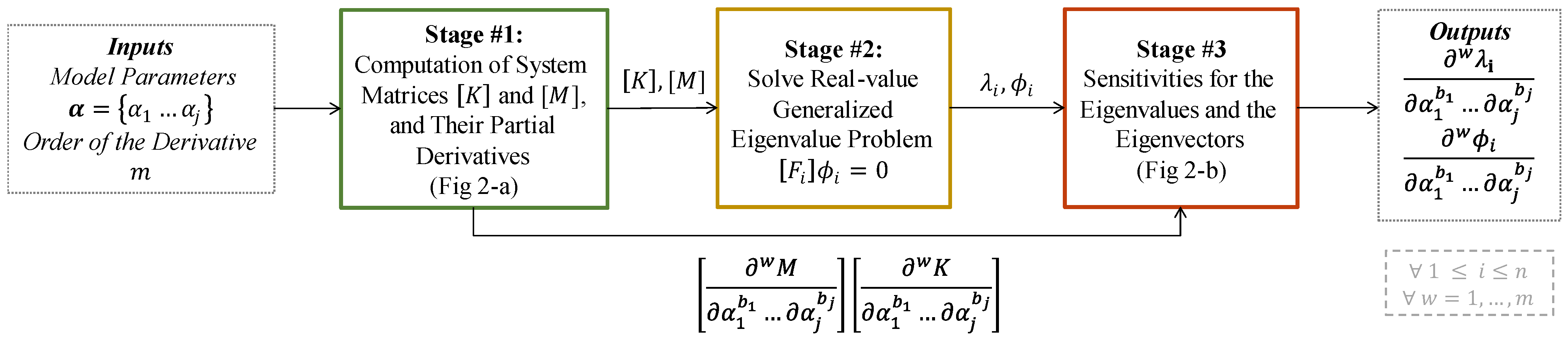
3. Sensitivity Analysis for Eigenfrequency Problems Using HYPAD

The methodology used to obtain arbitrary-order sensitivities of the eigenvalues and eigenvectors in eigenfrequency problems using HYPAD with multidual numbers is based on a process with three stages, as shown in the schematic in Figure 1. The main inputs required to perform the sensitivities calculation process are the maximum order of the derivative $m$ to be computed, and all the input parameters of the model ${=\{\alpha }_1$,$\dots ,{\alpha }_j\}$. In Stage 1, HYPAD is used to compute the system matrices $\left[K\right]$ and $\left[M\right]$, and their $m^{th}$ order sensitivities with respect to any input model parameter. In Stage 2, the matrices $\left[K\right]$ and $\left[M\right]$ are used to solve the traditional real-valued GEP for structural systems. Finally, in Stage 3, the sensitivities of $\left[K\right]$ and $\left[M\right]$ obtained from Stage 1 (e.g., $[{\partial }^{w}M/{(\partial {\alpha }_1^{b_1}\dots \partial {\alpha }_j^{b_j})]}^{}$ and $[{\partial }^{w}K/{(\partial {\alpha }_1^{b_1}\dots \partial {\alpha }_j^{b_j})]}^{}\forall w=1,\dots ,m$), and the eigenvalues and eigenvectors obtained from Stage 2 (e.g., ${\lambda }_i$ and ${\varphi }_i$,), are fed into a recursive subroutine that uses HYPAD to systematically expand Equations (3) and (4) to enable the computation of all the sensitivities of the eigenvalues and eigenvector up to order m. Below, a detailed description of each stage is presented:

Stage 1 is presented in Figure 2a and summarized as follows:

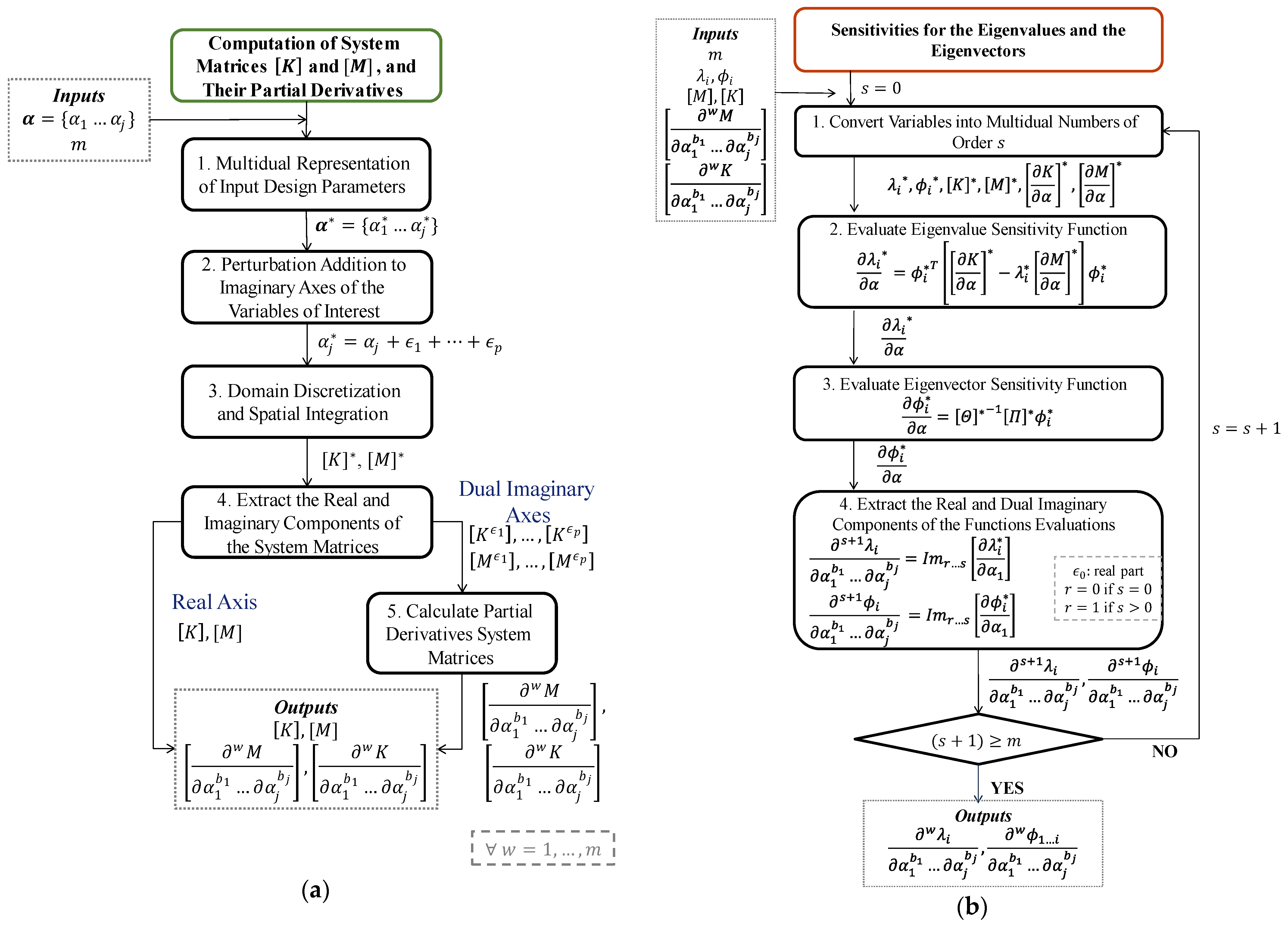
• The first step is to convert all the input parameters of the model into multidual variables of order m.
• Next, unitary perturbations, h, are added to the independent imaginary axes of the multidual axis of the specific variables for which the sensitivities want to be calculated. Here, adding perturbations to the same parameter in two different independent imaginary axes results in having second-order derivatives with respect to the perturbed parameter. Similarly, perturbing two different variables in two different independent imaginary axes results in crossed second-order derivatives. Following this logic, any combination of arbitrary-order sensitivities can be obtained.
• With the design parameters represented as multidual numbers and the appropriate perturbations applied, the structural system is discretized to obtain the global mass and stiffness matrices. Regardless of the discretization and spatial integration method used (e.g., FEM, BEM, SFEM, or others), when any input design parameter is represented as multidual and consequently perturbed, the mass and stiffness matrices will result in two $n x n$ multidual matrices ${\left[M\right]}^{*}$ and ${\left[K\right]}^{*}$. This approach is non-intrusive because the discretization and integration algorithms are unchanged; however, as the variables are multidual, algebraic operations are conducted using MultiZ.
• The next step in the methodology is to extract the real and imaginary information of ${\left[M\right]}^{*}$ and ${\left[K\right]}^{*}$ to form $p+1$ real matrices with dimensions $n\times n$, with $n$ being the number of DOF in the system, and $p$ is the number of dual imaginary axes. Each matrix corresponds to an axis on ${\left[M\right]}^{*}$ and ${\left[K\right]}^{*}$. The matrices obtained with the information from the real axes of ${\left[M\right]}^{*}$ and ${\left[K\right]}^{*},$ correspond to the global $[M$] and $[K$] matrices for the system and are identical to those obtained from a traditional real-variable analysis; while the matrices formed with the imaginary axes (e.g., $\left[K^{{ϵ}_1}\right]$,…, $\left[K^{{ϵ}_p}\right]$, and $\left[M^{{ϵ}_1}\right]$,…, $\left[M^{{ϵ}_p}\right]$) contain the information related to the partial derivatives of $\left[M\right]$ and $\left[K\right]$ with respect to the design input parameters that were perturbed.
• Finally, to complete the first stage, the derivatives of the system matrices are computed following Equation (7).

It must be highlighted that at the end of the first stage all the outputs are real variables. The dual variables are not passed to subsequent steps to simplify the algorithm.

Stage 2 consists of solving the real-value GEP described in Equation (1) to extract the system’s eigenvalues (${\lambda }_i$) and right eigenvectors with mass normalization (${\varphi }_i$). Here, any generalized eigensolver for self-adjoint problems can be applied. This constitutes a major advantage of the method since no hypercomplex-valued solvers are required. In addition, only the specific number of eigenvalues $i$, $\forall 1\le i\le n$ desired needs to be computed, avoiding the calculation of the whole basis of eigenvalues in the systems. Moreover, any eigenvalue and eigenvector derivative corresponding to any arbitrary mode can be calculated.

Stage 3 is presented in Figure 2b. This stage is based on a recursive algorithm controlled by the loop variable s that allows one to obtain the required sensitivities in ascending order up to the desired order $m$ using HYPAD. These recursive operations controlled by s are needed, because to obtain the sensitivities for order $s+1$ it is necessary to have solved the s-th order sensitivities for the eigenvalues and the eigenvectors. A description of the operations executed in Stage 3 is presented below, and an analytical demonstration of the use of HYPAD to obtain second-order sensitivities of eigenvalues and eigenvectors is presented in the Supplementary Material.

• The first step in Stage 3 is to convert ${\lambda }_i$, ${\varphi }_i$, $\left[M\right]$, [$K]$, [$\partial M/\partial \alpha ]$, and $[\partial K/\partial \alpha ]$ into multidual variables of order s. This procedure will allow the use of HYPAD to calculate the sensitivities. For instance, during the first iteration, when s = 0, the input parameters are converted into zero-order multidual numbers (i.e., multiduals of zero-order are real numbers). In subsequent iterations (e.g., s > 0), each imaginary axis of the multidual number contains the partial derivatives of the variables with respect to the input parameters of the model. In the case of the variables $[\partial K/\partial \alpha ]{}^{*}$ and [$\partial M/\partial \alpha ]{}^{*}$ that are already first-order sensitivities, the real part corresponds to the first-order sensitivities (e.g., [$\partial K/\partial \alpha ]$ and $[\partial M/\partial \alpha ]$), and the imaginary axes contain partial derivatives up to order $s+1$. In the case of ${\lambda }_i^{*}$ and ${\varphi }_i^{*}$, the real part corresponds to the eigenvalues and eigenvectors, and the imaginary axes are built from their derivatives with respect to the specific variables of interest. Note that the sensitivities for ${\lambda }_i$ and ${\varphi }_i$ up to order $s$ are always available because of the iterative nature of the procedure. Moreover, all combinations of partial derivatives of $\left[K\right]$ and $\left[M\right]$ are available from the first stage. More details on how to construct the multidual arrays are provided in the Supplementary Material, and the analytical demonstration in Section 4.
• With the multidual arrays, Equation (3) is evaluated, which results in a multidual variable ${\left(\partial {\lambda }_i/\partial \alpha \right)}^{*}$ that contains the first-order sensitivities in the real axis, and the $s+1$ order sensitivities in the dual imaginary axis. The expression evaluated at the multidual sampling points is:

  $$\begin{array}{c}{\frac{\partial {\lambda }_i}{\partial \alpha }}^{*}={{\varphi }_i^{*}}^T\left[{\left[\frac{\partial K}{\partial {\alpha }_{}^{}}\right]}^{*}-{\lambda }_i^{*}{\left[\frac{\partial M}{\partial {\alpha }_{}^{}}\right]}^{*}\right]{\varphi }_i^{*}\end{array}$$

  (10)
• Subsequently, using the same multidual arrays, Equation (4) is evaluated to calculate another multidual variable ${\left(\partial {\varphi }_i/\partial \alpha \right)}^{*}$. As for the eigenvalues, this variable contains in the real part, the first-order sensitivities of the eigenvectors, and in the dual imaginary axes, the $s+1$ sensitivities. The expression evaluated at the multidual sampling points is:

  $$\begin{array}{c}\frac{\partial {\varphi }_i^{\mathrm{*}}}{\partial \alpha }={{\left[\Theta \right]}^{\mathrm{*}}}^{-1}{\left[\Pi \right]}^{\mathrm{*}}{\varphi }_i^{\mathrm{*}}\end{array}$$

  (11)
• At this point, the $s+1$ order sensitivities of the eigenvalues and the eigenvectors lie in the imaginary axes of ${\left(\partial {\lambda }_i/\partial \alpha \right)}^{*}$ and ${\left(\partial {\varphi }_i/\partial \alpha \right)}^{*}$ found in step 2 and 3, respectively. Thus, to obtain the sensitivities, such coefficients are extracted by following the next rules. In the first iteration, when $s=0$, all the variables are multidual numbers of order zero (real numbers); therefore, this corresponds to a traditional first-order sensitivities calculation following the methodologies of Fox and Kapoor [17] and Yang and Peng [33]. In this case, the real part ($I{m}_0\left[\right]$) contains the sensitivity information. In subsequent iterations $(s>0)$, the $I{m}_{1\dots s}$[] is extracted, and the sensitivities are calculated by following Equation (7). To exemplify the specific axes that must be extracted on each pass through the loop, consider for instance the case of fourth-order sensitivities, the last iteration corresponds to $s=3$; therefore, the $I{m}_{1\dots 3}\left[\right]$ should be extracted, which corresponds to the ${Im}_{123}\left[\right]$ axis of the multidual number.

After completing the passes through the loop ($s+1\ge m$), all the sensitivities up to the desired order $m$ for any specific number of modes are available. In addition, all the lower-order mixed partial derivatives’ combinations are computed in the same process.

4. Sensitivity Analysis for Eigenfrequency Problems Using HYPAD

To illustrate the new methodology for obtaining arbitrary-order sensitivities in eigenfrequency problems using HYPAD, two simple application examples are presented: one is entirely analytical and corresponds to calculating the sensitivities for a simple mass and spring system. The other application example is numerical and corresponds to obtaining the sensitivities for the case of a free vibrating cantilever beam.

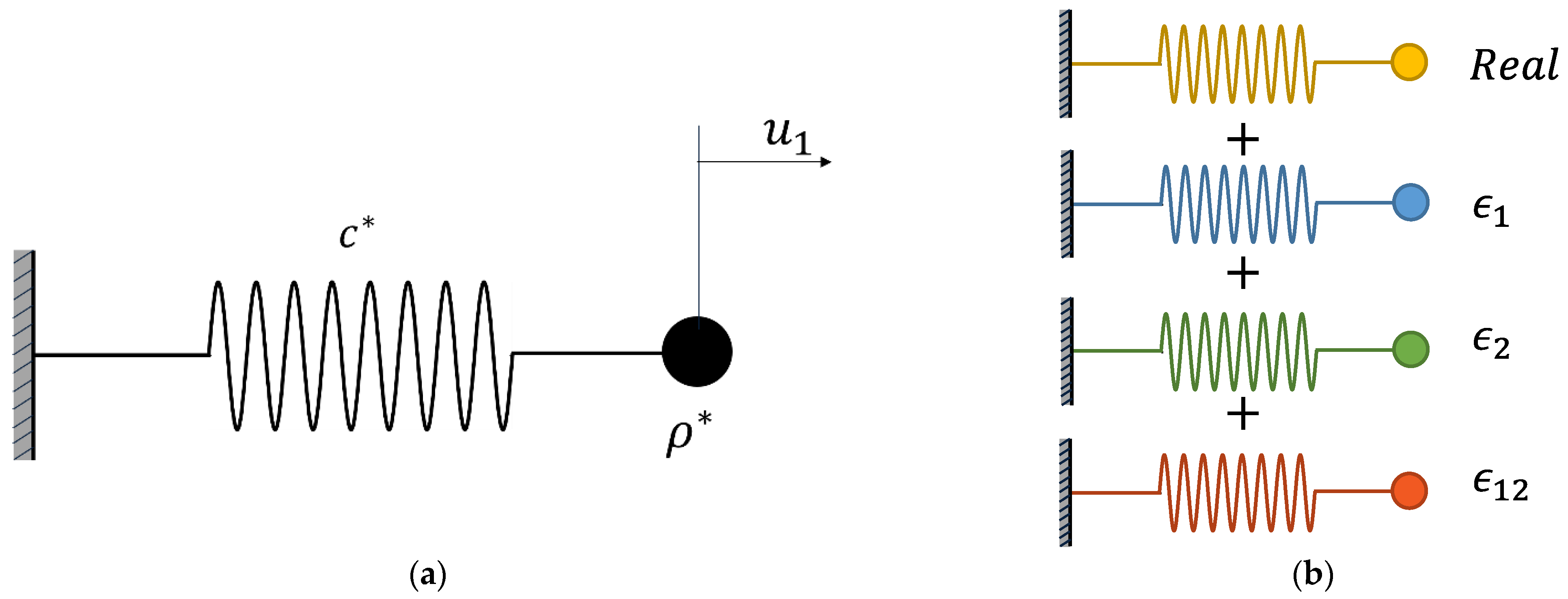
4.1. Simple Harmonic Oscillator

This example presents a step-by-step demonstration of the procedure introduced in Section 3 to obtain the mixed second-order partial derivatives for the simple harmonic oscillator shown in Figure 3a. The sensitivities were calculated with respect to the mass, $\rho$, and the spring stiffness, $c$. Due to the simplicity of the problem, all the steps can be calculated analytically.

The inputs for the algorithm presented in Figure 1 were the model parameters $\mathit{\alpha }=\{\rho ,c\}$, and the order of the derivative, in this case second-order $m=2$.

Stage 1

• For the case of mixed second-order sensitivities, both variables $\rho$ and $c$ must be converted into multidual arrays. In this case, bi-dual numbers are used with $p=3$. Therefore, three imaginary axes (e.g., ${ϵ}_1$, ${ϵ}_2$, and ${ϵ}_{12}$) are required. A graphical representation of this procedure is shown in Figure 3b.
• Next, to calculate mixed second-order partial derivatives with respect to $\rho$ and $c$, both variables are perturbed by applying a unitary step to the imaginary axes ${ϵ}_1$ and ${ϵ}_2$, respectively:

  $$\begin{array}{c}{\rho }^{*}={\rho }^{Re}+1{ϵ}_1+0{ϵ}_2+0{ϵ}_{12}\end{array}$$

  (12)

  $$\begin{array}{c}{c}^{*}=c^{Re}+0{ϵ}_1+1{ϵ}_2+0{ϵ}_{12}\end{array}$$

  (13)
• As this system corresponds to a one degree of freedom problem, no domain discretization and spatial integrations are necessary. Following the conventions from Figure 2, we have ${\left[M\right]}^{*}={\rho }^{*}$ and ${\left[K\right]}^{*}=c^{*}$.
• Consequently, the real components of the multidual variables ${\left[M\right]}^{*}$ and ${\left[K\right]}^{*}$ are extracted to form the following arrays:

  $$\begin{array}{c}\left[M\right]={Im}_0\left[{\left[M\right]}^{*}\right]=Real\left[{\left[M\right]}^{*}\right]{=\rho }^{Re}\end{array}$$

  (14)

  $$\begin{array}{c}\left[K\right]={Im}_0\left[{\left[K\right]}^{*}\right]=Real\left[{\left[K\right]}^{*}\right]=c^{Re}\end{array}$$

  (15)
• Similarly, the partial derivatives of $M$ and $K$ are obtained by evaluating Equation (7) using the information from the $p$ dual imaginary components of the multidual variables ${\left[M\right]}^{*}$ and ${\left[K\right]}^{*}$ as follows:

  $$\begin{array}{c}\frac{\partial M}{\partial {\rho }_{}}={Im}_1\left[{\left[M\right]}^{*}\right]={Im}_1\left[{\rho }^{Re}+1{ϵ}_1+0{ϵ}_2+0{ϵ}_{12}\right]=1\end{array}$$

  (16a)

  $$\begin{array}{c}\frac{\partial M}{\partial c}={Im}_2\left[{\left[M\right]}^{*}\right]={Im}_2\left[{\rho }^{Re}+1{ϵ}_1+0{ϵ}_2+0{ϵ}_{12}\right]=0\end{array}$$

  (16b)

  $$\begin{array}{c}\frac{{\partial }^{2}M}{\partial \rho \partial c}={Im}_{12}\left[{\left[M\right]}^{*}\right]={Im}_{12}\left[{\rho }^{Re}+1{ϵ}_1+0{ϵ}_2+0{ϵ}_{12}\right]=0\end{array}$$

  (16c)

  $$\begin{array}{c}\frac{\partial K}{\partial \rho }={Im}_1\left[{\left[K\right]}^{*}\right]={Im}_1\left[c^{Re}+0{ϵ}_1+1{ϵ}_2+0{ϵ}_{12}\right]=0\end{array}$$

  (17a)

  $$\begin{array}{c}\frac{\partial K}{\partial c}={Im}_2\left[{\left[K\right]}^{*}\right]={Im}_2\left[c^{Re}+0{ϵ}_1+1{ϵ}_2+0{ϵ}_{12}\right]=1\end{array}$$

  (17b)

  $$\begin{array}{c}\frac{{\partial }^{2}K}{\partial \rho \partial c}={Im}_{12}\left[{\left[K\right]}^{*}\right]={Im}_{12}\left[c^{Re}+0{ϵ}_1+1{ϵ}_2+0{ϵ}_{12}\right]=0\end{array}$$

  (17c)

Equations (14)–(17) constitute the output of Stage 1, which must be passed to the subsequent stages to calculate the eigenvalues’ and eigenvectors’ sensitivities.

Stage 2

Using the variables from Equations (14)–(15), the following generalized eigenvalue problem was solved:

$$\begin{array}{c}{\lambda }_1\left[{\rho }_{}^{Re}\right]{\left[{\varphi }_1^{Re}\right]}_{}=\left[c_{}^{RE}\right]\left[{\varphi }_1^{Re}\right]\end{array}$$

(18)

where the eigenvalue and mass normalized eigenvector correspond to:

$${\lambda }_1=c_{}^{Re}/{\rho }_{}^{Re}$$

(19a)

$${\varphi }_1={\left({\rho }_{}^{Re}\right)}^{-1/2}$$

(19b)

Stage 3

Iteration 1 ($s=0$): Following the procedure from Figure 2b, the loop variable is initialized from $s=0$.

• In this pass, multidual numbers of order zero (real numbers) were employed; therefore, the input variables $m=2,{\lambda }_1,{\varphi }_1,\left[M\right],\left[K\right],$ and the partial derivatives obtained in Stage 1 were kept as real numbers.
• The first-order sensitivities of the eigenvalues were obtained by evaluating Equation (3):

  $$\begin{array}{c}\frac{\partial {\lambda }_1}{\partial \rho }={\varphi }_1^T\left[\frac{\partial K}{\partial \rho }-{\lambda }_1\frac{\partial M}{\partial \rho }\right]{\varphi }_1=-\frac{c^{Re}}{{\left({\rho }_{}^{Re}\right)}^2}\end{array}$$

  (20)

  $$\begin{array}{c}\frac{\partial {\lambda }_1}{\partial c}={\varphi }_1^T\left[\frac{\partial K}{\partial c}-{\lambda }_1\frac{\partial M}{\partial c}\right]{\varphi }_1=\frac{1}{{\left({\rho }_{}^{Re}\right)}^{}}\end{array}$$

  (21)
• Similarly, the first-order sensitivities for the eigenvectors are obtained by evaluating Equation (4):

  $$\begin{array}{c}\frac{\partial {\varphi }_1}{\partial \rho }={\left[\left[K\right]-{\lambda }_1\left[M\right]+{\lambda }_1{\varphi }_1{\varphi }_1^T\left[M\right]\right]}^{-1}\left[\frac{\partial {\lambda }_1}{\partial \rho }\left[M\right]+{\lambda }_1\left[\frac{\partial M}{\partial \rho }\right]-\left[\frac{\partial K}{\partial \rho }\right]-\frac{1}{2}{{\varphi }_1^{}}^T\left[\frac{\partial M}{\partial \rho }\right]{\varphi }_1{\lambda }_1\right]=-\frac{1}{2\left({\left({\rho }_{}^{Re}\right)}^{3/2}\right)}\end{array}$$

  (22)

  $$\begin{array}{c}\frac{\partial {\varphi }_1}{\partial c}={\left[\left[K\right]-{\lambda }_1\left[M\right]+{\lambda }_1{\varphi }_1{{\varphi }_1^{}}^T\left[M\right]\right]}^{-1}\left[\frac{\partial {\lambda }_1}{\partial c}\left[M\right]+{\lambda }_1\left[\frac{\partial M}{\partial c}\right]-\left[\frac{\partial K}{\partial c}\right]-\frac{1}{2}{{\varphi }_1^{}}^T\left[\frac{\partial M}{\partial c}\right]{\varphi }_1{\lambda }_1\right]=0\end{array}$$

  (23)
• This case, which constitutes the first pass through the loop, does not require explicitly extracting the real parts from Equations (20)–(23); this is because, after the evaluation, the multidual number constitutes the first-order sensitivity per se.

Iteration 2 ($s=1$) The next iteration in the procedure (i.e., $s=1$) allows one to obtain the second-order sensitivities with respect to $\rho$ and $k$.

• All variables are first converted into multidual numbers of order one:

  $$\begin{array}{c}{\lambda }_1^{*}={\lambda }_1^{Re}+\frac{\partial {\lambda }_i}{\partial c}{ϵ}_1\end{array}$$

  (24a)

  $$\begin{array}{c}{\varphi }_1^{*}={\varphi }_1^{Re}+\frac{\partial {\varphi }_1}{\partial c}{ϵ}_1\end{array}$$

  (24b)

  $$\begin{array}{c}{\left[M\right]}^{*}={\rho }^{Re}+\frac{\partial M}{\partial c}{ϵ}_1\end{array}$$

  (24c)

  $$\begin{array}{c}{\left[K\right]}^{*}=c^{Re}+\frac{\partial K}{\partial c}{ϵ}_1\end{array}$$

  (24d)

  $$\begin{array}{c}\left[{\frac{\partial K}{\partial \rho }}^{*}\right]=\frac{\partial K}{\partial \rho }+\frac{\partial K}{\partial \rho \partial c}{ϵ}_1\end{array}$$

  (24e)

  $$\begin{array}{c}\left[{\frac{\partial M}{\partial \rho }}^{*}\right]=\frac{\partial M}{\partial \rho }+\frac{\partial M}{\partial \rho \partial c}{ϵ}_1\end{array}$$

  (24f)
• Then, the expression in Equation (3) is evaluated with the multidual arrays from Equation (24) as follows:

  $$\begin{array}{c}{\frac{\partial {\lambda }_1}{\partial \rho }}^{\mathrm{*}}={\left({\varphi }_1^{Re}+\frac{\partial {\varphi }_1}{\partial c}{ϵ}_1\right)}^T\left[\left[\frac{\partial K}{\partial \rho }+\frac{\partial K}{\partial \rho \partial c}{ϵ}_1\right]-\left({\lambda }_1^{Re}+\frac{\partial {\lambda }_i}{\partial c}{ϵ}_1\right)\left[\frac{\partial M}{\partial \rho }+\frac{\partial M}{\partial \rho \partial c}{ϵ}_1\right]\right]\left({\varphi }_1^{Re}+\frac{\partial {\varphi }_1}{\partial c}{ϵ}_1\right)\end{array}$$

  (25a)

  $$\begin{array}{c}{\frac{\partial {\lambda }_1}{\partial \rho }}^{\mathrm{*}}=-\frac{k}{{\left({\rho }^{Re}\right)}^2}-\frac{1}{{\left({\rho }^{Re}\right)}^2}{ϵ}_1\end{array}$$

  (25b)

Similarly, to calculate the second-order sensitivities of the eigenvectors, Equation (4) is evaluated (details of each term are provided in Appendix A) as:

$$\begin{array}{c}{\frac{\partial {\varphi }_1}{\partial \rho }}^{*}={{\left[\mathsf{\Theta }\right]}^{*}}^{-1}{\left[\mathsf{\Pi }\right]}^{*}{\varphi }_1^{*}\end{array}$$

(26a)

$$\begin{array}{c}{\frac{\partial {\varphi }_1}{\partial \rho }}^{*}=-\frac{1}{2\left({\left({\rho }_{}^{Re}\right)}^{3/2}\right)}+0{ϵ}_1\end{array}$$

(26b)

Then, the second-order sensitivity of the eigenvalue and the eigenvector is calculated by extracting the information from axis ${ϵ}_1$ in Equations (25b)–(26b) as:

$$\begin{array}{c}\frac{{\partial }^2{\lambda }_1}{\partial \rho \partial c}=-\frac{1}{{\left({\rho }_{}^{Re}\right)}^2}\end{array}$$

(27)

$$\begin{array}{c}\frac{{\partial }^2{\varphi }_1}{\partial \rho \partial c}=0\end{array}$$

(28)

Since the variable $s$ is exhausted, the stopping criteria is met, and the end of the algorithm is reached. Note that the expressions in Equations (25b)–(26b) contain, in the real axis, the information from the first-order sensitivity, which means that the arrays obtained at the end of the procedure in Figure 2b contain the arbitrary-order sensitivities and all the lower-order sensitivities. These results agree with the analytical equations presented in Appendix B.

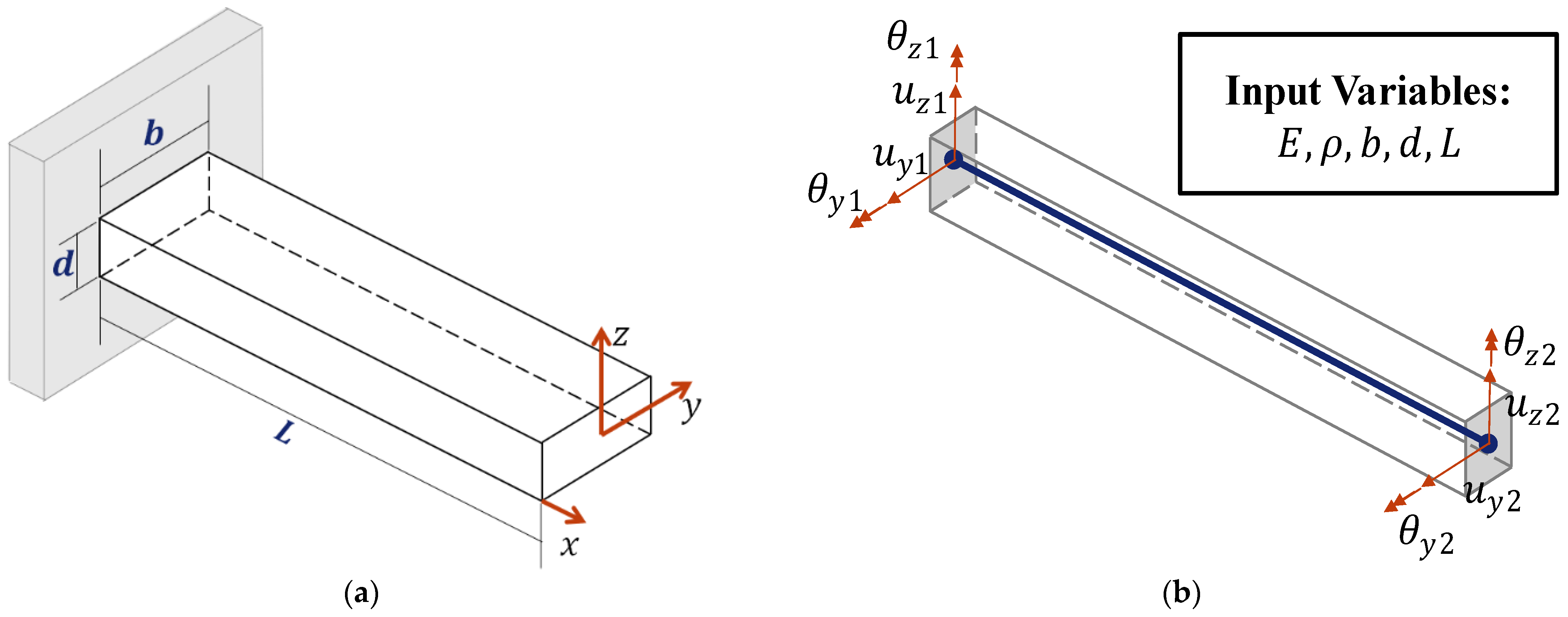
4.2. Free Vibration of a Cantilever Beam

The second example corresponds to a numerical implementation of the methodology for obtaining sensitivities in eigenfrequency problems using HYPAD. In this section, the methodology is applied to the analysis of the free vibration of a uniform elastic cantilever beam, illustrated in Figure 4a. The beam has a length $L$, stiffness $E$, mass density $\rho$, and a constant rectangular cross-sectional area $A$ with width $b$, and height $d$. The analytical expressions for the natural frequencies and shapes of the free vibration modes correspond to [76]:

$$\begin{array}{c}{\lambda }_i=\left\{\begin{array}{c}{{\lambda }_{iy}=\gamma }_i^4\frac{E{I}_y}{\rho A{L}^4}\\ {{\lambda }_{iz}=\gamma }_i^4\frac{E{I}_z}{\rho A{L}^4}\end{array}\right.where I_y=\frac{b{d}^3}{12},I_z=\frac{d{b}^3}{12},A=bd\end{array}$$

(29)

$$\begin{array}{c}{\varphi }_i\left(x\right)=\frac{1}{\sqrt{\rho AL}}\left[\frac{\left(\sinh \left({\gamma }_i\right)+\sin \left({\gamma }_i\right)\right)\left\{\cosh \left(\frac{{\gamma }_{i}x}{L}\right)-\cos \left(\frac{{\gamma }_{i}x}{L}\right)\right\}}{\sinh \left({\gamma }_i\right)+\sin \left({\gamma }_i\right)}-\frac{\left(\cosh \left({\gamma }_i\right)+\cos \left({\gamma }_i\right)\right)\left\{\sinh \left(\frac{{\gamma }_{i}x}{L}\right)-\sin \left(\frac{{\gamma }_{i}x}{L}\right)\right\}}{\sinh \left({\gamma }_i\right)+\sin \left({\gamma }_i\right)}\right]\end{array}$$

(30)

where ${\gamma }_i$ are given by:

$$\begin{array}{c}\cosh \left({\gamma }_i\right)\cos \left({\gamma }_i\right)+1=0\hspace{1em}\hspace{1em}\hspace{1em}\forall \left(i=\mathrm{1,2},\dots \right)\end{array}$$

(31)

The three first roots of Equation (31) are:

$${\gamma }_1=1.8751\hspace{1em}{\gamma }_2=4.6941\hspace{1em}{\gamma }_3=7.8547$$

Since the beam has two axes of symmetry (i.e., y and z), the eigenvalues will appear alternated in the analytical solution. Therefore, the modes will be classified between those in the y-direction as ${\lambda }_{iy}$, and those in the z-direction as ${\lambda }_{iz}$. The system can have repeated or distinct eigenvalues depending on the characteristics of the cross-sectional area. The first case of repeated eigenvalues is evident in symmetric cross-sections when the cross-section has the same first moment of area with respect to two or more axes. For instance, for a square cross-section, the inertia in directions y and z are the same; therefore, ${\lambda }_{iy}={\lambda }_{iz}$. On the contrary, if a non-symmetric cross-section is used, as in the case of a rectangle cross-section, the inertia in y and z are different; therefore, ${\lambda }_{iy}\ne {\lambda }_{iz}$. Here, both situations are considered.

The methodology was implemented in FORTRAN using the LAPACK [77] library to solve the GEP and to obtain the eigenvectors with mass normalization using the procedure described in Figure 1a. The code is made available to the reader as Supplementary Material to the article. Up to third-order sensitivities ($m=3$) were computed with respect to the material and geometrical parameters for the first six natural modes of the cantilevered beam. As an initial step, the parameters of the model ($E,\rho ,L,b$ and $d$) were transformed into their corresponding multidual representation to become $E^{*},{\rho }^{*},L^{*},b^{*}$ and $d^{*}$, depending on the derivatives calculated in each case. Subsequently, unit perturbations were added along the different multidual imaginary axes of the variables depending on the specific sensitivities that were to be calculated. The beam was discretized using standard Euler–Bernoulli elements, with each node containing four DOF, two translational and two rotational, as shown in Figure 4b. A total of one hundred equal-length Euler–Bernoulli elements were used. The element stiffness ${\left[K^e\right]}^{*}$ and mass ${\left[M^e\right]}^{*}$ matrices were calculated by using the multidual variables and the formulation in Equations (32)–(33), respectively. In addition, the global mass and stiffness matrices were assembled following a traditional finite element method scheme.

$$\begin{array}{c}{\left[K^e\right]}^{*}=\frac{E^{*}}{L^{*}}\left[\begin{array}{cccccccc}\frac{12I_z^{*}}{{L^{*}}^2}& 0& 0& \frac{6I_z^{*}}{L^{*}}& -\frac{12I_z^{*}}{{L^{*}}^2}& 0& 0& \frac{6I_z^{*}}{L^{*}}\\ 0& \frac{12I_y^{*}}{{L^{*}}^2}& -\frac{6I_y^{*}}{L^{*}}& 0& 0& -\frac{12I_y^{*}}{{L^{*}}^2}& -\frac{6I_y^{*}}{L^{*}}& 0\\ 0& -\frac{6I_y^{*}}{L^{*}}& 4I_y^{*}& 0& 0& \frac{6I_y^{*}}{L^{*}}& 2I_y^{*}& 0\\ \frac{6I_z^{*}}{L^{*}}& 0& 0& 4I_z^{*}& -\frac{6I_z^{*}}{L^{*}}& 0& 0& 2I_z^{*}\\ -\frac{12I_z^{*}}{{L^{*}}^2}& 0& 0& -\frac{6I_z^{*}}{L^{*}}& \frac{12I_z^{*}}{{L^{*}}^2}& 0& 0& -\frac{6I_z^{*}}{L^{*}}\\ 0& -\frac{12I_y^{*}}{{L^{*}}^2}& \frac{6I_y^{*}}{L^{*}}& 0& 0& \frac{12I_y^{*}}{{L^{*}}^2}& \frac{6I_y^{*}}{L^{*}}& 0\\ 0& -\frac{6I_y^{*}}{L^{*}}& 2I_y^{*}& 0& 0& \frac{6I_y^{*}}{L^{*}}& 4I_y^{*}& 0\\ \frac{6I_z^{*}}{L^{*}}& 0& 0& 2I_z^{*}& -\frac{6I_z^{*}}{L^{*}}& 0& 0& 4I_z^{*}\end{array}\right]\end{array}$$

(32)

where $I_z^{\mathrm{*}}=d^{\mathrm{*}}{b^{\mathrm{*}}}^3$/12, and $I_y^{\mathrm{*}}={d^{\mathrm{*}}}^3{b}^{\mathrm{*}}/12$.

$$\begin{array}{c}{\left[M^e\right]}^{*}=\frac{{\rho }^{*}{A}^{*}{L}^{*}}{420}\left[\begin{array}{cccccccc}156& 0& 0& 22L^{*}& 54& 0& 0& -13L^{*}\\ 0& 156& -22L^{*}& 0& 0& 54& 13L^{*}& 0\\ 0& -22L^{*}& 4{L^{*}}^2& 0& 0& -13L^{*}& -3{L^{*}}^2& 0\\ 22L^{*}& 0& 0& 4{L^{*}}^2& 13L^{*}& 0& 0& -3{L^{*}}^2\\ 54& 0& 0& 13L^{*}& 156& 0& 0& -22L^{*}\\ 0& 54& -13L^{*}& 0& 0& 156& 22L^{*}& 0\\ 0& 13L^{*}& -3{L^{*}}^2& 0& 0& 22L^{*}& 4{L^{*}}^2& 0\\ -13L^{*}& 0& 0& -3{L^{*}}^2& -22L^{*}& 0& 0& 4{L^{*}}^2\end{array}\right]\end{array}$$

(33)

where $A^{\mathrm{*}}=d^{\mathrm{*}}{b}^{\mathrm{*}}$.

Subsequently, the boundary conditions were defined for the multidual matrices ${\left[K\right]}^{*}$ and ${\left[M\right]}^{*}$, eliminating the real and dual imaginary DOF under homogeneous Dirichlet boundary conditions. Then, the information from each imaginary axis of the multidual arrays was extracted to form $p=7$ matrices corresponding to each of the dual imaginary axes of the tridual number. The matrices $\left[K\right]$ and $\left[M\right]$ constructed from the information of the real axis were used to solve the GEP and obtain the eigenvalues and eigenvectors. In addition, the information from the dual imaginary axes was used to calculate the partial derivatives of the system matrices by following Equation (7). Then, as described in Figure 2b, the eigenvalues ${\lambda }_i$, the eigenvectors ${\varphi }_i$ for $i=1,\dots ,6$, $m=3,$ the system matrices $\left[K\right]$ and $\left[M\right]$, and their partial derivatives, were used to calculate the sensitivities of the eigenvalues and eigenvectors. Three iterations were processed through the algorithm in Stage 3.

The relative percentage error (RE) described in Equation (34) was used to measure the error for each of the eigenvalues and their sensitivities. For the eigenvectors, an average of the RE was used as an error measurement. For both measures of error, the analytical solutions in Equations (29)–(30) were used as a reference.

$$\begin{array}{c}RE=\frac{\left|y_j^{Analytical}-y_j^{ZTSE}\right|}{\left|y_j^{Analytical}\right|}\end{array}$$

(34)

A semi-analytical demonstration was conducted to illustrate the present verification problem for the reader. In this case, the cantilever beam was discretized using a single Euler–Bernoulli element. Although such a small number of elements does not achieve convergence and the stability of the results, it shows a step-by-step demonstration of the methodology. An example can be found in the Supplementary Material.

4.2.1. Sensitivity Analysis of a Cantilever Beam with Distinct Eigenvalues

A cantilever beam was analyzed with properties $L=5 \mathrm{m}, E=68.9 \mathrm{G}\mathrm{P}\mathrm{a}, \rho =2770 \mathrm{k}\mathrm{g}{\mathrm{m}}^{-3}, b=0.01 \mathrm{m}$ and $d=0.015 \mathrm{m}$. The characteristics of the cross-section area yielded distinct eigenvalues. Higher-order sensitivities with respect to the material ($E$, $\rho$) and geometrical ($L$) input design parameters were calculated. Three specific cases are presented, each representing an independent pass throughout the whole methodology. Third-order sensitivities with respect to the density $\rho$, third-order sensitivities with respect to the length of the beam $L$, and mixed third-order sensitivities with respect to the three parameters. This requires using tri-dual numbers with $p=7$ imaginary axes. In the first case, perturbations were added only to $\rho$ on its three independent dual imaginary axes, becoming ${\rho }^{*}=2770+{ϵ}_1+{ϵ}_2+{ϵ}_3$. In the second case, perturbations were added only to $L$ on its three independent dual imaginary axes, becoming $L^{*}=5+{ϵ}_1+{ϵ}_2+{ϵ}_3.$ In the third case, the perturbations were added to the three variables, these becoming ${\rho }^{*}=2770+{ϵ}_1$, $E^{*}=68\times {10}^9+{ϵ}_2$ and $L^{*}=5+{ϵ}_3$. The axes not displayed here contain a value of zero for all cases.

Table 1. Natural Frequencies of the first six modes for a Cantilever Beam with a Rectangular Cross-Sectional Area (Distinct Eigenvalues).

Mode i	${\mathit{\lambda }}_{\mathit{i}}$ (%Error $\times {10}^{-8}$)
1	4.100 (92.390)
2	9.225 (2.775)
3	$161.022$ (1.616)
4	362.299 (0.842)
5	1262.435 (5.348)
6	2840.480 (5.243)

shows the results corresponding to the eigenvalues and Figure 5 the results for the eigenvectors. Excellent agreement is found between the analytical solution and the numerical estimates, resulting in a maximum RE of $9.239\times {10}^{-7}\%$ in the eigenvalues, and an average RE of $2.750\times {10}^{-6}\%$ for the eigenvectors.

Table 2. Eigenvalue sensitivity with respect to the density for a system with distinct eigenvalues. The subscripts imply derivation.

Mode i	${\mathit{\lambda }}_{\mathit{i},\mathit{\rho }}\times {10}^{-2}$ $(\mathbf{\%}\mathbf{E}\mathbf{r}\mathbf{r}\mathbf{o}\mathbf{r}\times 10^{-8})$	${\mathit{\lambda }}_{\mathit{i},\mathit{\rho }\mathit{\rho }}\times {10}^{-5}$ ($\mathbf{\%}\mathbf{E}\mathbf{r}\mathbf{r}\mathbf{o}\mathbf{r}\times 10^{-8}$)	${\mathit{\lambda }}_{\mathit{i},\mathit{\rho }\mathit{\rho }\mathit{\rho }}\times {10}^{-8}$ ($\mathbf{\%}\mathbf{E}\mathbf{r}\mathbf{r}\mathbf{o}\mathbf{r}\times 10^{-8}$)
1	$-0.1480$ (92.390)	$0.107$ (93.180)	$-0.116$ (93.716)
2	$-0.333$ (2.775)	$0.240$ (2.806)	$-0.260$(2.826)
3	$-5.813$ (1.616)	$4.197$ (1.620)	$-4.545$ (1.623)
4	$-13.079$ (0.842)	$9.444$ (0.842)	$-10.228$ (0.843)
5	$-45.575$ (5.348)	$32.906$ (5.348)	$-35.639$ (5.348)
6	$-102.540$ (5.243)	$74.039$ (5.243)	$-80.187$ (5.243)

,

Table 3. Eigenvalue sensitivity to the beam length for a system with distinct eigenvalues. The subscripts imply derivation.

Mode i	${\mathit{\lambda }}_{\mathit{i},\mathit{L}}\times {10}^2$ $(\mathbf{\%}\mathbf{E}\mathbf{r}\mathbf{r}\mathbf{o}\mathbf{r}\times 10^{-8})$	${\mathit{\lambda }}_{\mathit{i},\mathit{L}\mathit{L}}\times {10}^2$ $(\mathbf{\%}\mathbf{E}\mathbf{r}\mathbf{r}\mathbf{o}\mathbf{r}\times 10^{-8})$	${\mathit{\lambda }}_{\mathit{i},\mathit{L}\mathit{L}\mathit{L}}\times {10}^2$ $(\mathbf{\%}\mathbf{E}\mathbf{r}\mathbf{r}\mathbf{o}\mathbf{r}\times 10^{-8})$
1	$-0.0328$ (23.643)	$0.0328$ (11.605)	$-0.0394$ (6.725)
2	$-0.0738$ (2.916)	$0.0738$ (0.827)	$-0.0885$ (0.216)
3	$-1.288$ (0.883)	$1.288$ (0.791)	$-1.5458$ (0.739)
4	$-2.898$ (0.683)	$2.898$ (0.691)	$-3.478$ (0.696)
5	$-10.099$ (5.308)	$10.099$ (5.295)	$-12.119$ (5.290)
6	$-22.724$ (5.276)	$22.724$ (5.282)	$-27.269$ (5.284)

and

Table 4. Eigenvalue sensitivity with respect to Young’s Modulus and mixed partial derivatives for a system with distinct eigenvalues. The subscripts imply derivation.

Mode i	${\mathit{\lambda }}_{\mathit{i},\mathit{E}}\times {10}^{-9}$ $(\mathbf{\%}\mathbf{E}\mathbf{r}\mathbf{r}\mathbf{o}\mathbf{r}\times 10^{-8})$	${\mathit{\lambda }}_{\mathit{i},\mathit{E}\mathit{\rho }}\times {10}^{-13}$ $(\mathbf{\%}\mathbf{E}\mathbf{r}\mathbf{r}\mathbf{o}\mathbf{r}\times 10^{-8})$	${\mathit{\lambda }}_{\mathit{i},\mathit{E}\mathit{\rho }\mathit{L}}\times {10}^{-13}$ $(\mathbf{\%}\mathbf{E}\mathbf{r}\mathbf{r}\mathbf{o}\mathbf{r}\times 10^{-8})$
1	0.0595 (0.0911)	−0.215 (0.107)	0.172 (0.831)
2	0.134 (0.137)	−0.483 (0.178)	0.3866 (0.585)
3	2.337 (0.679)	−8.436 (0.679)	6.750 (0.689)
4	5.258 (0.672)	−18.983 (0.671)	15.187 (0.675)
5	18.323 (5.286)	−66.147 (5.286)	52.918 (5.286)
6	2578 (5.285)	−148.830 (5.285)	119.060 (5.285)

and Figure 6 show the results of the sensitivity analysis of the structure. A good agreement is found with a maximum percentual error of $9.371\times {10}^{-7}$% in the sensitivities of the eigenvalues and an average RE of $7.066\times {10}^{-6}$% for the eigenvectors. These results preserve the same error magnitudes as the real solution, reflecting that HYPAD does not induce truncation nor subtraction cancellation errors. In addition, the same behavior is found for all the sensitivities regardless of the parameter of interest. Other combinations of sensitivities are presented in the Supplementary Material.

4.2.2. Cantilever Beam with Repeated Eigenvalues

A model with symmetries about two rotational axes was studied to demonstrate our methodology when the system exhibits repeated eigenvalues. Here, a square cross-sectional area cantilever beam with $L=5 \mathrm{m},E=68.9 \mathrm{G}\mathrm{P}\mathrm{a},\rho =2770 \mathrm{k}\mathrm{g}{\mathrm{m}}^{-3},b=0.01 \mathrm{m},$ and $b=d=0.01 \mathrm{m}$ was considered. High-order sensitivities with respect to geometrical global and directional design variables were calculated. The first case corresponded to variables whose derivatives are also repeated because the symmetry of the system was not altered. On the other hand, directional design variables correspond to variables that affect the symmetry of the system; therefore, regardless of having repeated eigenvalues, their sensitivities are not repeated.

Table 5. Natural Frequencies of the first six modes for a Cantilever Beam with a Rectangular Cross-Sectional Area (Distinct Eigenvalues).

Mode i	${\mathit{\lambda }}_{\mathit{i}}$ (%Error $\times 10^{-8})$
1, 2	4.100 (75.618)
3, 4	161.020 (1.152)
5, 6	1262.400 (5.330)

shows the results for the eigenvalues of the system. The eigenvectors are shown in Figure 7. As in the previous example, good agreement is found between the analytical solution and the numerical estimates, resulting in a maximum RE of $7.562\times {10}^{-7}$% for the eigenvalues and an average of 0.0499% for the eigenvectors.

5. Global Design Variable

Sensitivities with respect to the global input design parameters were calculated. The material parameters, such as $E$ and $\rho$, and the geometry parameters $L$ and $b$ were considered global design variables. Third-order sensitivities were calculated with respect to $b$. In this case, the variable $b$ is perturbed the same amount in both directions ($y$ and $z$) to achieve a global sensitivity (no breakage of symmetry). Thereby, $b$ is perturbed to become $b^{*}=0.01+{ϵ}_1+{ϵ}_2+{ϵ}_3.$ In addition, third-order mixed partial derivatives were calculated with respect to $\rho$, $L$ and $b$. In this case, perturbations must be added to the three variables, these becoming ${\rho }^{*}=2770+{ϵ}_1$, $L^{*}=5+{ϵ}_2$, and $b^{*}=0.01+{ϵ}_3$.

Table 6. Sensitivities for a system with repeated eigenvalues. The subscripts imply derivation.

Mode i.	${\mathit{\lambda }}_{\mathit{i},\mathit{b}}\times {10}^4$ (%Error $\times 10^{-8})$	${\mathit{\lambda }}_{\mathit{i},\mathit{b}\mathit{b}}\times {10}^6$ (%Error $\times 10^{-8})$	${\mathit{\lambda }}_{\mathit{i},\mathit{b}\mathit{b}\mathit{b}}$ (%Error $\times 10^{-8})$
1, 2	0.0819 (67.996)	0.0819 (213.889)	0.00
3, 4	3.220 (0.250)	3.220 (0.207)	0.00
5, 6	25.249 (5.231)	25.249 (5.502)	0.00

and

Table 7. Mixed higher-order sensitivities for a system with repeated eigenvalues. The subscripts imply derivation.

Mode i	${\mathit{\lambda }}_{\mathit{i},\mathit{\rho }\mathit{b}}$ (%Error $\times 10^{-8})$	${\mathit{\lambda }}_{\mathit{i},\mathit{b}\mathit{L}}\times {10}^4$ (%Error $\times 10^{-8})$	${\mathit{\lambda }}_{\mathit{i},\mathit{\rho }\mathit{L}\mathit{b}}$ (%Error $\times 10^{-8})$
1, 2	−0.296 (68.632)	−0.0655 (19.942)	0.236 (19.657)
3, 4	−11.626 (0.247)	−2.576 (0.619)	9.301 (0.621)
5, 6	−91.150 (5.231)	−20.189 (5.280)	72.920 (5.280)

show the results for the sensitivity analysis. Good agreement was found between the numerical results and the analytical solution, with a maximum RE of $2.139\times {10}^{-6}$% for the eigenvalues. In this case, the same behavior of the error observed for the distinct eigenvalues case is present. These results validate, again, the inexistence of truncation and subtractive cancellation errors when differentiating using HYPAD with multidual numbers because the order of magnitude of the errors is preserved.

Figure 8 shows the results for the eigenvector sensitivities; a good agreement was found between the numerical results and the analytical solutions. The maximum average RE was found to be equal to 0.199%.

6. Directional Design Variables (Geometrical)

Sensitivities were calculated for the case of directional variables. In the present problem, the only directional input design variables are the cross-section parameter $d$ and $b,$ which are analogous. In this case, sensitivities were calculated with respect to $d$. This variable only affects the eigenvalues associated with $I_y$; thus, the sensitivities of some modes are zero, as seen in

Table 8. Eigenvalue sensitivity to the width of the cross-sectional area for a system with repeated eigenvalues. The subscripts imply derivation.

Mode i	${\mathit{\lambda }}_{\mathit{i},\mathit{d}}\times {10}^4$ (%Error $\times 10^{-8})$	${\mathit{\lambda }}_{\mathit{i},\mathit{d}\mathit{d}}\times {10}^6$ (%Error $\times 10^{-8})$
1	0.0819 (11.746)	0.0819 (23.098)
2	0.000	0.000
3	3.220 (0.856)	3.220 (0.383)
4	0.000	0.000
5	25.249 (5.260)	25.249 (5.334)
6	0.000	0.000

. Here, the variable $d$ is perturbed to become $d^{*}=0.01+{ϵ}_1+{ϵ}_2$. Table 8 shows the results for the sensitivity analysis. Good agreement was found between the numerical results and the analytical solution with a maximum relative error of $2.310\times {10}^{-7}$% for the eigenvalues.

Figure 9 shows the results of the first- and second-order sensitivities of the eigenvectors reflecting good agreement when compared against the analytical solutions. The average RE of $0.496\%$ was equal for both sensitivities. Although the sensitivities of the eigenvalues are distinct for each of the modes the sensitivities of the eigenvectors are equal for each pair of modes, and the methodology can recover this behavior.

7. Perturbation Step Size Converge Analysis

To demonstrate the capacity of our proposed method to obtain highly accurate sensitivities, we performed a convergence study of the perturbation step size for the case of distinct eigenvalues and compared it with FD. Figure 10a–c shows the variability in the relative error measurement for the derivatives of the eigenvalues corresponding to the first mode of vibration. Notably, the error for HYPAD remains constant regardless of the chosen step size for analysis. In contrast, the FD results exhibit high variability concerning the step size. Initially, the error decreases with the value of the step size up to an optimal point; then, as the step size keeps decreasing, the error starts to become dominated by the subtractive cancellation error, increasing its nominal value. Furthermore, the error with FD amplifies with the order of the derivative, resulting in errors with magnitudes of ${10}^{10}$. In the method proposed here, the error in any arbitrary-order sensitivity is in the same order as that of the real solution. The Supplementary Material presents the same analysis for the higher vibration modes.

8. Discussion

The methodology presented in this paper enables the calculation of arbitrary-order sensitivities of eigenvalues and eigenvectors using HYPAD. In this case, multidual numbers were used to compute the sensitivities with high accuracy. The methodology is grounded on the works presented by Fox and Kapoor [17] and Yang and Peng [33] and formulated for self-adjoint systems. Although the focus of this work was on the analysis of structural dynamical systems, without loss of generality, the same methodology could be applied to other types of physics described by the GEP (e.g., Buckling analysis, principal component analysis (PCA), etc.).

The method was developed for the case of distinct and repeated eigenvalues and showed high accuracy for both types of problems when compared to repeated form analytical solutions in free vibration analysis of a cantilever beam. In the mathematical development of the equation to compute eigenvectors’ sensitivities [33], it is stated that the matrix $\left[\mathsf{\Theta }\right]$ can become singular in some cases when eigenvalues of high multiplicity (repeated, with several similar eigenvalues) are obtained. Despite this, no sign of singularity has been observed in the verification analysis performed in this work. However, a more in-depth analysis is needed in future to present a more in-depth conclusion.

The implementation of the current approach into commercial structural analysis software (i.e., Abaqus, Ansys, etc.) is left as future work. This could allow an increase in computational efficiency and enable the widespread use of the method for general structural systems regardless of the number of degrees of freedom. Although multidual numbers were used in this research to eliminate both truncation and subtractive cancellation errors, traditional complex numbers can be used if the user requires only the computation of first-order sensitivities, which are available in most of the commercial programming platforms. The only consideration needed is that the perturbation step size $h$ should be small, say $\approx {10}^{-10}$ times the variable of interest.

The proposed methodology is limited to analyzing the linear dynamics response of structural systems and does not consider the effect of material non-linearities, damping, loading or geometrical non-linearities. In addition, the computational cost, in terms of time and memory consumption, is acknowledged as a limitation of the proposed methodology. This limitation arises from the loss of sparsity and memory when evaluating the matrix of the coefficients in Equation (4). The issue becomes particularly challenging in systems with a large number of input design parameters, as it requires solving numerous systems of equations to assess all combinations of higher-order derivatives. To address this limitation, we are actively developing a solution that involves implementing a local residual formulation capable of computing sensitivities from expressions derived at the elemental level. This new formulation aims to preserve the sparsity of the matrix of coefficients. By adopting this strategy, we anticipate significant improvements in the efficiency and scalability of our methodology.

9. Conclusions

A novel methodology was developed and demonstrated to accurately calculate higher-order sensitivities of the eigenvalues and eigenvectors for eigenfrequency problems using the hypercomplex automatic differentiation (HYPAD) method. The method integrates HYPAD with exact semi-analytical expressions developed from differentiating the equations of the generalized eigenvalue problem, and to compute arbitrary-order sensitivities of the structural matrices. Sensitivities with respect to the material and geometrical parameters were obtained and verified for the analysis of the free vibration of a discrete cantilever beam with a known analytical solution. Two types of problems were analyzed: (i) a model with distinct eigenvalues, and (ii) a model with repeated eigenvalues, with high accuracy in both cases. The advantages of this approach are that both truncation and subtractive errors are eliminated from the sensitivity analysis, and a single general expression is used for the computation of the sensitivities of both eigenvalues and eigenvectors up to arbitrary-order. This results in accurate and efficient sensitivity results. In this case, the error of the sensitivities is dependent upon the error of the numerical method used to solve the generalized eigenvalue problem, which can be further reduced with mesh refinements.

An additional advantage of the presented methodology is given by the possibility of evaluating higher-order sensitivities for only a specific number of modes, not altogether as happens with other approaches. This is beneficial; since, in large systems, finding the spectrum of eigenvalues and eigenvectors is known to be expensive. In addition, the HYPAD method can calculate all higher-order sensitivities with respect to all the input model parameters using only one function evaluation, which makes it easy to implement in commercial practice. Finally, regardless of the hypercomplex nature of the operations used to calculate the sensitivities, the method presented here uses real only numbers when solving the generalized eigenvalue problem. This is crucial since no commercial hypercomplex eigensolver is currently available. In the future, if hypercomplex solvers become available, that could impose the need to reformulate the methodology.

Multiple applications of the higher-order sensitivities are envisioned to perform a sensitivity analysis in structural systems. As examples, the sensitivities can be used to improve the performance of topology optimization models, finite element updating algorithms, and other algorithms where accurate derivatives are crucial to correctly guide the processes. Further research efforts will be focused on implementing the present methodology within commercial structural analysis software to include the calculation of sensitivities in damped systems.

References

1. Ruiz, D.; Bellido, J.C.; Donoso, A. Eigenvector sensitivity when tracking modes with repeated eigenvalues. Comput. Methods Appl. Mech. Eng. 2017, 326, 338–357. [Google Scholar] [CrossRef]
2. Lin, R.M.; Ng, T.Y. New theoretical developments on eigenvector derivatives with repeated eigenvalues. Mech. Syst. Signal Process. 2019, 129, 677–693. [Google Scholar] [CrossRef]
3. Zhong, W.; Cheng, G. Second-Order Sensitivity Analysis of Multimodal Eigenvalues and Related Optimization Techniques. J. Struct. Mech. 1986, 14, 421–436. [Google Scholar] [CrossRef]
4. Lin, R.M.; Mottershead, J.E.; Ng, T.Y. A state-of-the-art review on theory and engineering applications of eigenvalue and eigenvector derivatives. Mech. Syst. Signal Process. 2020, 138, 106536. [Google Scholar] [CrossRef]
5. Mottershead, J.E.; Link, M.; Friswell, M.I. The sensitivity method in finite element model updating: A tutorial. Mech. Syst. Signal Process. 2011, 25, 2275–2296. [Google Scholar] [CrossRef]
6. Yoon, G.H.; Donoso, A.; Carlos Bellido, J.; Ruiz, D. Highly efficient general method for sensitivity analysis of eigenvectors with repeated eigenvalues without passing through adjacent eigenvectors. Int. J. Numer. Methods Eng. 2020, 121, 4473–4492. [Google Scholar] [CrossRef]
7. Pryse, S.E.; Kundu, A.; Adhikari, S. Projection methods for stochastic dynamic systems: A frequency domain approach. Comput. Methods Appl. Mech. Eng. 2018, 338, 412–439. [Google Scholar] [CrossRef] [Green Version]
8. Francis, J.G.F. The QR Transformation A Unitary Analogue to the LR Transformation—Part 1. Comput. J. 1961, 4, 265–271. [Google Scholar] [CrossRef] [Green Version]
9. Francis, J.G.F. The QR Transformation—Part 2. Comput. J. 1962, 4, 332–345. [Google Scholar] [CrossRef] [Green Version]
10. Sorensen, D.C. Implicit Application of Polynomial Filters in a k-Step Arnoldi Method. SIAM J. Matrix Anal. Appl. 1992, 13, 357–385. [Google Scholar] [CrossRef] [Green Version]
11. Davidson, E.R. The iterative calculation of a few of the lowest eigenvalues and corresponding eigenvectors of large real-symmetric matrices. J. Comput. Phys. 1975, 17, 87–94. [Google Scholar] [CrossRef]
12. Andrew, A.L. Iterative Computation of Derivatives of Eigenvalues and Eigenvectors. IMA J. Appl. Math. 1979, 24, 209–218. [Google Scholar] [CrossRef]
13. Tan, R.C.E.; Andrew, A.L. Computing Derivatives of Eigenvalues and Elgenvectors by Simultaneous Iteration. IMA J. Numer. Anal. 1989, 9, 111–122. [Google Scholar] [CrossRef]
14. Tan, R.C.E. Some acceleration methods for iterative computer of derivatives of eigenvalues and eigenvectors. Int. J. Numer. Methods Eng. 1989, 28, 1505–1519. [Google Scholar] [CrossRef]
15. Burchett, B.T.; Costello, M. QR-based algorithm for eigenvalue derivatives. AIAA J. 2002, 40, 2319–2322. [Google Scholar] [CrossRef]
16. Wittrick, W.H. Rates of Change of Eigenvalues, With Reference to Buckling and Vibration Problems. J. R. Aeronaut. Soc. 1962, 66, 590–591. [Google Scholar] [CrossRef]
17. Fox, R.L.; Kapoor, M.P. Rates of change of eigenvalues and eigenvectors. AIAA J. 1968, 6, 2426–2429. [Google Scholar] [CrossRef]
18. Rogers, L.C. Derivatives of eigenvalues and eigenvectors. AIAA J. 1970, 8, 943–944. [Google Scholar] [CrossRef]
19. Plaut, R.H.; Huseyin, K. Derivatives of eigenvalues and eigenvectors in non-self-adjoint systems. AIAA J. 1973, 11, 250–251. [Google Scholar] [CrossRef]
20. Rudisill, C.S. Derivatives of eigenvalues and eigenvectors for a general matrix. AIAA J. 1974, 12, 721–722. [Google Scholar] [CrossRef]
21. Jankovic, M.S. Exact nth derivatives of eigenvalues and eigenvectors. J. Guid. Control. Dyn. 1994, 17, 136–144. [Google Scholar] [CrossRef]
22. Garza, J.; Millwater, H.R. Multicomplex Newmark-Beta Time Integration Method for Sensitivity Analysis in Structural Dynamics. AIAA J. 2015, 53, 1188–1198. [Google Scholar] [CrossRef]
23. Lim, K.B.; Junkins, J.L.; Wang, B.P. Re-examination of eigenvector derivatives. J. Guid. Control. Dyn. 1987, 10, 581–587. [Google Scholar] [CrossRef]
24. Iott, J.; Haftka, R.; Adelman, H.M. Selecting Step Sizes in Sensitivity Analysis by Finite Differences. No. NASA-TM-86382. 1985. Available online: https://ntrs.nasa.gov/citations/19850025225 (accessed on 24 May 2023).
25. Wang, B.P.; Apte, A.P. Complex variable method for eigensolution sensitivity analysis. AIAA J. 2006, 44, 2958–2961. [Google Scholar] [CrossRef]
26. Navarro, J.D.; Millwater, H.R.; Montoya, A.H.; Restrepo, D. Arbitrary-Order Sensitivity Analysis in Phononic Metamaterials Using the Multicomplex Taylor Series Expansion Method Coupled with Bloch’s Theorem. J. Appl. Mech. 2021, 89, 021007. [Google Scholar] [CrossRef]
27. Fujikawa, M.; Tanaka, M.; Mitsume, N.; Imoto, Y. Hyper-dual number-based numerical differentiation of eigensystems. Comput. Methods Appl. Mech. Eng. 2022, 390, 114452. [Google Scholar] [CrossRef]
28. Zhang, D.; Wei, F.-S. Computation of eigenvector derivatives with repeated eigenvalues using a complete modal space. AIAA J. 1995, 33, 1749–1753. [Google Scholar] [CrossRef]
29. Nelson, R.B. Simplified calculation of eigenvector derivatives. AIAA J. 1976, 14, 1201–1205. [Google Scholar] [CrossRef]
30. Zhao, Y.; Liu, Z.; Chen, S.; Zhang, G. An accurate modal truncation method for eigenvector derivatives. Comput. Struct. 1999, 73, 609–614. [Google Scholar] [CrossRef]
31. Balmes, E. Efficient sensitivity analysis based on finite element model reduction. In Proceedings of the International Modal Analysis Conference—IMAC, Santa Barbara, CA, USA, 2–5 February 1998; Volume 2, pp. 1118–1124. [Google Scholar]
32. Bernard, M.L.; Bronowicki, A.J. Modal expansion method for eigensensitivity with repeated roots. AIAA J. 1994, 32, 1500–1506. [Google Scholar] [CrossRef]
33. Yang, Q.; Peng, X. An exact method for calculating the eigenvector sensitivities. Appl. Sci. 2020, 10, 2577. [Google Scholar] [CrossRef] [Green Version]
34. Ojalvo, I.U. Efficient computation of modal sensitivities for systems with repeated frequencies. AIAA J. 1988, 26, 361–366. [Google Scholar] [CrossRef]
35. Dailey, R.L. Eigenvector derivatives with repeated eigenvalues. AIAA J. 1989, 27, 486–491. [Google Scholar] [CrossRef]
36. Li, Z.; Lai, S.K.; Wu, B. A new method for computation of eigenvector derivatives with distinct and repeated eigenvalues in structural dynamic analysis. Mech. Syst. Signal Process. 2018, 107, 78–92. [Google Scholar] [CrossRef]
37. Wu, B.S.; Xu, Z.H.; Li, Z.G. Improved nelson’s method for computing eigenvector derivatives with distinct and repeated eigenvalues. AIAA J. 2007, 45, 950–952. [Google Scholar] [CrossRef]
38. Friswell, M.I. The Derivatives of Repeated Eigenvalues and Their Associated Eigenvectors. J. Vib. Acoust. 1996, 118, 390–397. [Google Scholar] [CrossRef]
39. Song, D.; Han, W.; Chen, S.; Qiu, Z. Simplified calculation of eigenvector derivatives with repeated eigenvalues. AIAA J. 1996, 34, 859–862. [Google Scholar] [CrossRef]
40. Friswell, M.I. Calculation of second and higher order eigenvector derivatives. J. Guid. Control. Dyn. 1995, 18, 919–921. [Google Scholar] [CrossRef]
41. Bernard, J.E.; Kwon, S.K.; Wilson, J.A. Differentiation of mass and stiffness matrices for high order sensitivity calculations in finite element-based equilibrium problems. ASME. J. Mech. Des. 1993, 115, 829–832. [Google Scholar] [CrossRef]
42. Long, X.Y.; Jiang, C.; Han, X. New method for eigenvector-sensitivity analysis with repeated eigenvalues and eigenvalue derivatives. AIAA J. 2015, 53, 1226–1235. [Google Scholar] [CrossRef]
43. Seyranian, A.P.; Lund, E.; Olhoff, N. Multiple eigenvalues in structural optimization problems. Struct. Optim. 1994, 8, 207–227. [Google Scholar] [CrossRef]
44. Cheng, G.; Olhoff, N. Rigid body motion test against error in semi-analytical sensitivity analysis. Comput. Struct. 1993, 46, 515–527. [Google Scholar] [CrossRef]
45. Olhoff, N.; Rasmussen, J.; Lund, E. A Method of “Exact” Numerical Differentiation for Error Elimination in Finite-Element-Based Semi-Analytical Shape Sensitivity Analyses. Mech. Struct. Mach. 1993, 21, 1–66. [Google Scholar] [CrossRef]
46. Olhoff, N.; Lund, E. Finite Element Based Engineering Design Sensitivity Analysis and Optimization. In Advances in Structural Optimization: Solid Mechanics and Its Applications; Herskovits, J., Ed.; Springer: Dordrecht, The Netherlands, 1995; Volume 25. [Google Scholar] [CrossRef]
47. Bletzinger, K.U.; Firl, M.; Daoud, F. Approximation of derivatives in semi-analytical structural optimization. Comput. Struct. 2008, 86, 1404–1416. [Google Scholar] [CrossRef]
48. Lantoine, G.; Russell, R.P.; Dargent, T. Using Multicomplex Variables for Automatic Computation of High-Order Derivatives. ACM Trans. Math. Softw. 2012, 38, 1–21. [Google Scholar] [CrossRef]
49. Fike, J.; Alonso, J. The Development of Hyper-Dual Numbers for Exact Second-Derivative Calculations. In Proceedings of the 49th AIAA Aerospace Sciences Meeting including the New Horizons Forum and Aerospace Exposition, Orlando, FL, USA, 4–7 January 2011; American Institute of Aeronautics and Astronautics: Reston, VA, USA, 2011. [Google Scholar]
50. Voorhees, A.; Millwater, H.; Bagley, R. Complex variable methods for shape sensitivity of finite element models. Finite Elem. Anal. Des. 2011, 47, 1146–1156. [Google Scholar] [CrossRef]
51. Voorhees, A.; Millwater, H.; Bagley, R.; Golden, P. Fatigue sensitivity analysis using complex variable methods. Int. J. Fatigue 2012, 40, 61–73. [Google Scholar] [CrossRef]
52. Voorhees, A.; Bagley, R.; Millwater, H.; Golden, P. Application of Complex Variable Methods for Fatigue Sensitivity Analysis. In Proceedings of the 50th AIAA/ASME/ASCE/AHS/ASC Structures, Structural Dynamics, and Materials Conference, Palm Springs, CA, USA, 4–7 May 2009; American Institute of Aeronautics and Astronautics: Reston, VA, USA, 2009. [Google Scholar]
53. Montoya, A.; Millwater, H. Sensitivity analysis in thermoelastic problems using the complex finite element method. J. Therm. Stress. 2017, 40, 302–321. [Google Scholar] [CrossRef]
54. Balzani, D.; Gandhi, A.; Tanaka, M.; Schröder, J. Numerical calculation of thermo-mechanical problems at large strains based on complex step derivative approximation of tangent stiffness matrices. Comput. Mech. 2015, 55, 861–871. [Google Scholar] [CrossRef]
55. Ramirez Tamayo, D.; Montoya, A.; Millwater, H. A virtual crack extension method for thermoelastic fracture using a complex-variable finite element method. Eng. Fract. Mech. 2018, 192, 328–342. [Google Scholar] [CrossRef]
56. Wagner, D.; Garcia, M.J.; Montoya, A.; Millwater, H. A finite element-based adaptive energy response function method for 2D curvilinear progressive fracture. Int. J. Fatigue 2019, 127, 229–245. [Google Scholar] [CrossRef]
57. Ramirez-Tamayo, D.; Soulami, A.; Gupta, V.; Restrepo, D.; Montoya, A.; Millwater, H. A complex-variable cohesive finite element subroutine to enable efficient determination of interfacial cohesive material parameters. Eng. Fract. Mech. 2021, 247, 107638. [Google Scholar] [CrossRef]
58. Montoya, A.; Fielder, R.; Gomez-Farias, A.; Millwater, H. Finite-Element Sensitivity for Plasticity Using Complex Variable Methods. J. Eng. Mech. 2015, 141, 04014118. [Google Scholar] [CrossRef]
59. Hürkamp, A.; Tanaka, M.; Kaliske, M. Complex step derivative approximation of consistent tangent operators for viscoelasticity based on fractional calculus. Comput. Mech. 2015, 56, 1055–1071. [Google Scholar] [CrossRef]
60. Fielder, R.; Montoya, A.; Millwater, H.; Golden, P. Residual stress sensitivity analysis using a complex variable finite element method. Int. J. Mech. Sci. 2017, 133, 112–120. [Google Scholar] [CrossRef]
61. Gomez-Farias, A.; Montoya, A.; Millwater, H. Complex finite element sensitivity method for creep analysis. Int. J. Press. Vessel. Pip. 2015, 132–133, 27–42. [Google Scholar] [CrossRef]
62. Monsalvo, J.F.; García, M.J.; Millwater, H.; Feng, Y. Sensitivity analysis for radiofrequency induced thermal therapies using the complex finite element method. Finite Elem. Anal. Des. 2017, 135, 11–21. [Google Scholar] [CrossRef]
63. Fielder, R.; Millwater, H.; Montoya, A.; Golden, P. Efficient estimate of residual stress variance using complex variable finite element methods. Int. J. Press. Vessel. Pip. 2019, 173, 101–113. [Google Scholar] [CrossRef]
64. Tanaka, M.; Fujikawa, M.; Balzani, D.; Schröder, J. Robust numerical calculation of tangent moduli at finite strains based on complex-step derivative approximation and its application to localization analysis. Comput. Methods Appl. Mech. Eng. 2014, 269, 454–470. [Google Scholar] [CrossRef]
65. Chun, J. Sensitivity analysis of system reliability using the complex-step derivative approximation. Reliab. Eng. Syst. Saf. 2021, 215, 107814. [Google Scholar] [CrossRef]
66. Smith, D.E.; Siddhi, V. Generalized Approach for Incorporating Normalization Conditions in Design Sensitivity Analysis of Eigenvectors. AIAA J. 2006, 44, 2552–2561. [Google Scholar] [CrossRef]
67. Wedderburn, J.H.M. On Hypercomplex Numbers. Proc. Lond. Math. Soc. 1908, s2-6, 77–118. [Google Scholar] [CrossRef]
68. Eastham, M.S.P. 2968. On the definition of dual numbers. Math. Gaz. 1961, 45, 232–233. [Google Scholar] [CrossRef]
69. Balcer, M.R.; Millwater, H.; Favorite, J.A. Multidual Sensitivity Method in Ray-Tracing Transport Simulations. Nucl. Sci. Eng. 2021, 195, 907–936. [Google Scholar] [CrossRef]
70. Kantor, I.L.; Kantor, I.L.; Solodovnikov, A.S. Hypercomplex Numbers: An Elementary Introduction to Algebras; Springer: New York, NY, USA, 1989. [Google Scholar]
71. Martins, J.R.R.A.; Sturdza, P.; Alonso, J.J. The connection between the complex-step derivative approximation and algorithmic differentiation. ACM Trans. Math. Softw. 2001, 46, 23. [Google Scholar] [CrossRef] [Green Version]
72. Millwater, H.R.; Shirinkam, S. Multicomplex Taylor Series Expansion For Computing High-Order Derivatives. Int. J. Apllied Math. 2014, 27, 311–334. [Google Scholar] [CrossRef] [Green Version]
73. Aguirre-Mesa, A.M.; Garcia, M.J.; Millwater, H. MultiZ: A library for computation of high order derivatives using multicomplex or multidual numbers. ACM Trans. Math. Softw. 2020, 46, 1–30. [Google Scholar] [CrossRef]
74. Price, G.B. An Introduction to Multicomplex Spaces and Functions; Dekker: New York, NY, USA, 1991. [Google Scholar]
75. Aguirre-Mesa, A.M.; Garcia, M.J.; Aristizabal, M.; Wagner, D.; Ramirez-Tamayo, D.; Montoya, A.; Millwater, H. A block forward substitution method for solving the hypercomplex finite element system of equations. Comput. Methods Appl. Mech. Eng. 2021, 387, 114195. [Google Scholar] [CrossRef]
76. Bottega, W.J. Engineering Vibrations; Taylor & Francis: Abingdon, UK, 2006. [Google Scholar]
77. Anderson, E.; Bai, Z.; Bischof, C.; Blackford, S.; Demmel, J.; Dongarra, J.; Du Croz, J.; Greenbaum, A.; Hammarling, S.; McKenney, A.; et al. {LAPACK} Users’ Guide; Society for Industrial and Applied Mathematics: Philadelphia, PA, USA, 1999. [Google Scholar]
Figure 1. General methodology used to compute arbitrary-order sensitivities of the eigenvalues and eigenvectors using HYPAD.
Applsci 13 07125 g001
Figure 2. Flowchart for the sensitivity analysis of eigenfrequency problems using HYPAD. (a) Stage 1: General procedure used to compute the sensitivities of eigenvalues and eigenvectors. (b) Stage 3: Details on the process used to calculate the sensitivities of the eigenvalues and eigenvectors using HYPAD and semi-analytical expressions.
Applsci 13 07125 g002
Figure 3. (a) Schematic representation of the hypercomplex masses and spring system. (b) Schematic representation of the different axes of the multidual representation of the mass-spring discrete model.
Applsci 13 07125 g003
Figure 4. (a) Schematic of the cantilever beam for the free vibration system; (b) Finite element formulation for standard Euler–Bernoulli elements.
Applsci 13 07125 g004
Figure 5. Natural shape modes for a Cantilever Beam with a Rectangular Cross-Sectional Area (Distinct Eigenvalues). Solid Black lines represent the analytical solution, red represents the first and second mode, magenta the third and fourth mode, and green the fifth and sixth mode.
Applsci 13 07125 g005
Figure 6. Eigenvector sensitivities with respect to material properties and geometry parameters. Solid black lines represent the analytical solution, red represents the first and second mode, magenta the third and fourth mode, and green the fifth and sixth mode.
Applsci 13 07125 g006aApplsci 13 07125 g006b
Figure 7. Natural Modes for a Cantilever Beam with a Squared Cross-Sectional Area (Repeated Eigenvalues). Solid black lines represent the analytical solution, red represents the first and second mode, magenta the third and fourth mode, and green the fifth and sixth mode.
Applsci 13 07125 g007
Figure 8. Eigenvector sensitivities with respect to the global geometric parameters. Solid black lines represent the analytical solution, red represents the first and second mode, magenta the third and fourth mode, and green the fifth and sixth mode.
Applsci 13 07125 g008aApplsci 13 07125 g008b
Figure 9. Eigenvector sensitivities with respect to directional geometric parameters. Solid black lines represent the analytical solution, red represents the first and second mode, magenta the third and fourth mode, and green the fifth and sixth mode.
Applsci 13 07125 g009
Figure 10. Step size refinement for the first mode of vibration. The dashed line represents the results from HYPAD and the solid line the results from FD. (a) First-order derivatives. (b) Second-order derivatives. (c) Third-order derivatives.
Applsci 13 07125 g010