Application of Feedforward Cascade Compound Control Based on Improved Predictive Functional Control in Heat Exchanger Outlet Temperature System

Abstract

Aiming at the problems of large delay and poor anti-disturbance ability in the outlet temperature control system of the heat exchanger to optimize the control accuracy of the system and improve the control performance, this paper proposes a control scheme combining predictive functional control with proportional-integral-derivative control. Using the incremental proportional-integral-derivative control algorithm to improve the optimization objective function of the predictive functional control algorithm, a predictive functional control optimization model with a proportional-integral-derivative structure is established. The feedforward compensation control is adopted to eliminate the influence of external disturbances on the heat exchanger temperature control system. Through simulation, the proposed control scheme is compared with the feedforward cascade compound control scheme based on a proportional-integral-derivative main controller. The results show that the scheme has a small over harmonic and strong anti-interference ability. The adaptability and stability of the system are significantly improved, and the exit temperature of the heat exchanger can be effectively controlled.

1. Introduction

At present, one of the main purposes of designing control strategies in the field of industrial processes is to improve energy efficiency. More than 80% of the world’s energy use today involves heat transfer processes [1]. The heat exchanger is a common piece of heat transfer equipment in the chemical production process. It is also called a heat exchanger, which uses the heat exchange between cold and hot fluids to ensure that the temperature of the liquid after heating meets the needs of the process so that production can be carried out smoothly [2]. Choosing a reasonable control scheme can not only control the outlet temperature of the heat exchanger but also improve heat transfer efficiency and provide economic benefits [3,4,5,6,7]. The performance of the control system has a great influence on the economic efficiency of the process, and the control performance can usually be improved by applying advanced control algorithms [8,9,10].

The most commonly used control strategy in the field of industrial process control is proportional-integral-derivative (PID) control. Since 1936, experts and scholars have proposed many PID tuning methods [11]. But how to determine the appropriate PID parameters is still a question worthy of discussion [12]. In industrial control, the appropriate PID adjustment method is generally selected according to the model type, such as the first-order plus dead time (FOPDT) model [13,14], integrator plus dead time (IPDT) model [15,16], etc. In industrial production, the PID control scheme is generally used to control the system. However, for the process dynamic model with a time-varying and large lag, the traditional PID control can’t eliminate the obvious overshoot in the control, has a long adjustment time, and can’t solve the problem of time-varying control model parameters.

Since 1970, model predictive control (MPC) has been proposed and developed, and it has a good control effect on complex optimization problems [17]. However, when dealing with nonlinear, uncertain, and time-varying control systems, MPC control alone is still relatively laborious. Furthermore, MPC is not as easy to implement as PID control. Therefore, it is very necessary to find a way to effectively combine MPC and PID control. Vasičkaninová et al. combined neural network predictive control (NNPC) and fuzzy control in the outlet temperature control of heat exchangers. The simulation results demonstrate the effectiveness and superiority of the complex control structure, which combines NNPC and an auxiliary fuzzy controller [18]. Czeczot et al. applied balancing-based adaptive control (BBAC) to a simple heat distribution system and showed that the method ensured better anti-jamming capability compared with the traditional PI controller [19]. Bakošová et al. proposed a predictive control strategy based on a simplified model-based heat exchange network approach [20]. Carvalho et al. proposed an advanced technique based on artificial neural network model predictive control (NNMPC) and compared it with two PIDs and a linear MPC controller in simulation [21]. Oravec et al. took the time-varying parameters of the heat exchanger as parameter uncertainty and adopted robust MPC to deal with the process with uncertainty [22]. In

Table 1. The main content of the study.

References	Type of Heat Exchanger	Control Scheme	Result
Vasičkaninová et al. [18]	Tubular	The NN predictive control combined with the auxiliary fuzzy P controller	The advantage of this approach is that it is not a linear-model-based strategy and the control input constraints are directly included in the controller synthesis. And the scheme provides satisfactory control responses for the set-point tracking as well as for the disturbance rejection.
Czeczot et al. [19]	Plate	The balance-based adaptive control methodology	The simulation results of the control scheme show that even in the case when there is no feedforward action in the final form of the control law, the B-BAC methodology ensures good control properties, without any steady state bias of the regulation error.
Bakošová et al. [20]	Shell-and-tube	Robust model predictive control	In the presence of uncertainty and boundaries on control inputs and controlled outputs, the robust feedback control approach reduced the steady-state offsets of the petroleum temperature in the outlet streams from the HEs by approximately 40–50% compared with the LQ optimal control.
Carvalho et al. [21]	Shell-and-tube	neural network MPC	Simulation experiments in servo and regulatory tests showed that the NNMPC assured a smooth control response in set-point tracking. Moreover, the controller presented the smallest overshoots in the disturbance rejection experiment.
Oravec et al. [22]	shell-and-tube	Robust model predictive control with integral action	This controller was used for control of the shell-and-tube heat exchangers and the simulation results confirmed that robust MPC with integral actions ensured offset-free control performance.

, the main findings of the studies are provided.

The predictive functional control (PFC) algorithm, as the third generation of the MPC control algorithm, differs from the traditional MPC algorithm in that it is a structured control input [23]. It introduces the concept of basis function, and its output response can be obtained through offline calculation in advance, thereby reducing the workload of the computer that needs to be solved online and improving work efficiency.

In this paper, the PFC algorithm is combined with the PID control algorithm, and the incremental PID control algorithm is used to improve the optimization objective function of the PFC algorithm so that the controller has the structural characteristics of proportional, integral, and derivative. Compared with the single algorithm, the improved PFC (IPFC) control algorithm has the advantages of fast response and high control precision. At the same time, a feedforward cascade compound control scheme based on IPFC is proposed for the three measurable but uncontrollable disturbance quantities, namely, the flow rate of hot fluid, the inlet temperature of hot fluid, and the inlet temperature of the refrigerant. The feedforward control is used to eliminate the influence of the main interference on the outlet temperature, and the other interference is controlled by feedback. The simulation results show that the method can effectively reduce the overshoot of the system, has good anti-interference, and greatly improves the control performance of the heat exchanger temperature control system.

The main contribution of this paper is to propose a cascaded forward control scheme based on IPFC. Firstly, an improved predictive functional control algorithm is proposed. Secondly, according to the other three controllable input variables of the heat exchanger: refrigerant inlet temperature, hot fluid flow, and hot fluid inlet temperature, the disturbance compensation of these three main interference variables is carried out by the feedforward control method to eliminate the influence of the main external interference on the heat exchanger outlet temperature. In the current research on heat exchanger outlet temperature control, the common feedforward control scheme only selects one main interference variable to compensate, but in this paper, we will consider the three main interference variables. Finally, the simulation shows the suppression effect of the control system on the three disturbance variables under model matching. The suppression effect of the control system on interference when the interference channel model is mismatched and the suppression effect of the control system on interference when the main controlled object model is mismatched. The control scheme proposed in this paper will provide a reference for the research of the heat exchanger outlet temperature control system to suppress interference.

The organizational structure of this article is as follows. In Section 1, the research status of the heat exchanger outlet temperature control system is introduced. In Section 2, the mathematical model of the heat exchanger is established using mechanism modeling. In Section 3, an improved predictive functional control algorithm is introduced. In Section 4, a feedforward cascade compound control scheme based on an improved predictive functional control algorithm is proposed. In Section 5, simulation and experimental analysis are presented. In Section 6, there is a discussion of future work. Section 7, is the conclusion of this paper.

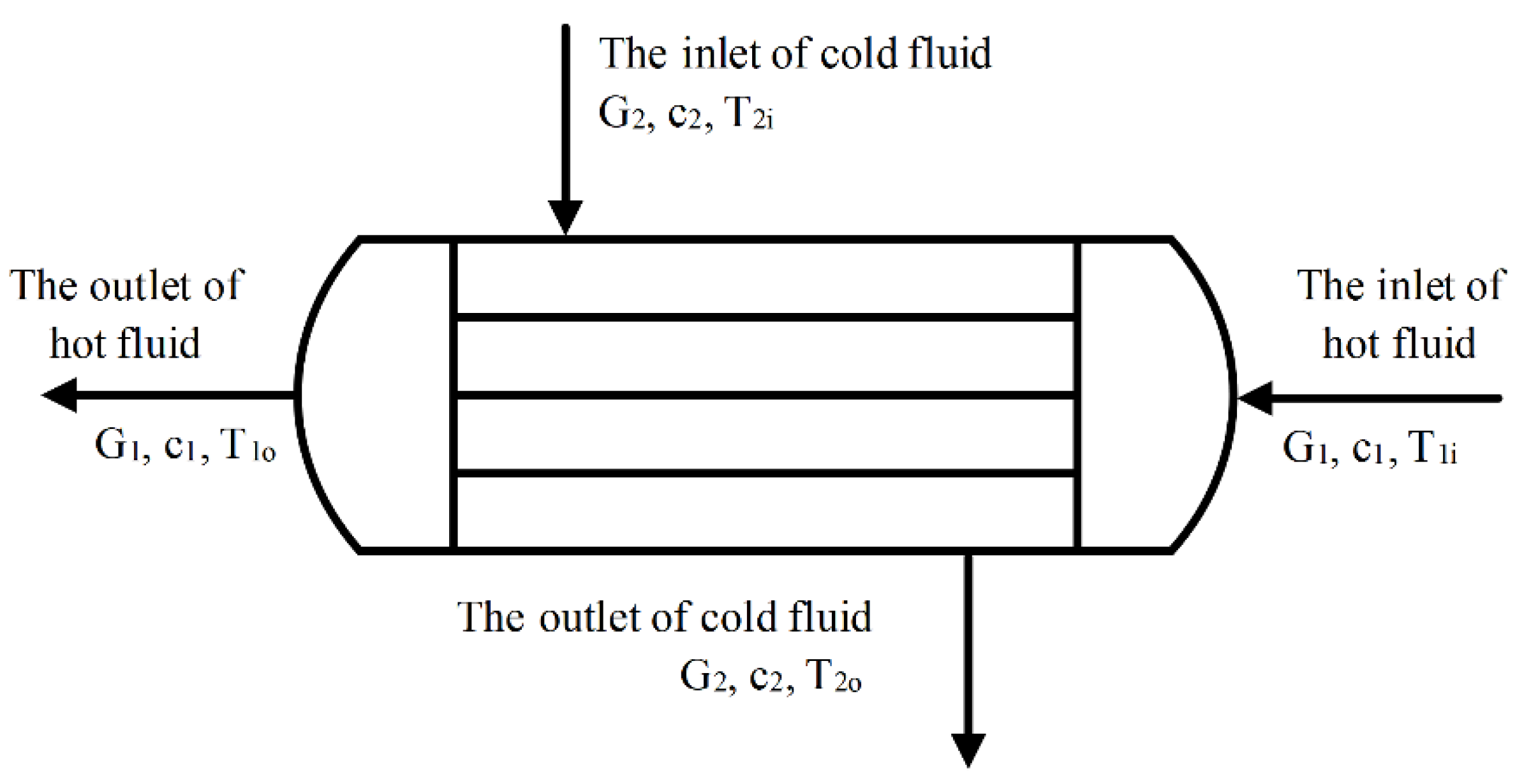
2. Heat Exchanger Model

In this paper, the heat exchanger model is established in the form of a countercurrent single-pass tube, and its mathematical model is established through the analysis of static and dynamic characteristics [24]. The structure diagram of the heat exchanger is shown in Figure 1. In this case, the product is hot water, and the heat-transfer fluid is cold water. The product enters the exchanger at a flow rate G₁ and temperature $T_{1i}$ and leaves at a temperature $T_{1o}$. At the opposite end of the device, the heat-transfer fluid enters with a flow rate G₂ and temperature $T_{2i}$ and exits with a temperature $T_{2o}$. The objective is to regulate the temperature of the output fluid, the product, by acting on the counter-current flow rate of the “heat-transfer fluid”.

2.1. Static Characteristic Analysis

Static characteristics in a process control system are defined as the relationship between controlled parameters and control variables in a steady state, which can be described by the corresponding algebraic equations. The static characteristic equation of the heat exchanger temperature control system can be derived from the two basic equations of the heat transfer process, namely, Equations (1) and (2).

$$q=G_2{c}_2\left(T_{2i}-T_{2o}\right)=G_1{c}_1\left(T_{1o}-T_{1i}\right)$$

(1)

where, $q$ refers to the heat transfer rate, the unit is $\mathrm{w}$; G₁ and G₂ refer to the mass flow of hot and cold liquids, kg/s; c₁ and c₂ are the average specific heat capacities of hot and cold liquids, the unit is $\mathrm{J}/\left(\mathrm{kg}·°\mathrm{C}\right)$; $T_{1i}$ and $T_{1o}$ are the hot liquid inlet and outlet temperatures, $T_{2i}$ and $T_{2o}$ are the cold liquid inlet and outlet temperatures, the unit is °C.

The heat transfer rate $q$ from a hot liquid to a cold liquid is given by the heat transfer theorem:

$$q=KF\Delta T$$

(2)

where, K refers to the heat transfer coefficient, $\mathrm{w}/\left({\mathrm{m}}^2·°\mathrm{C}\right)$; F refers to the heat transfer area, ${\mathrm{m}}^2$; $\Delta T$ means average temperature difference, °C.

The average temperature difference $\Delta T$ is represented by the logarithmic average:

$$\Delta T=\frac{\left(T_{2i}-T_{1o}\right)-\left(T_{2o}-T_{1i}\right)}{\ln \frac{T_{2i}-T_{1o}}{T_{2o}-T_{1i}}}=\frac{\Delta t_1-\Delta t_2}{\ln \frac{\Delta t_1}{\Delta t_2}}$$

(3)

where,

$$\left\{\begin{array}{c}\Delta t_1=T_{2i}-T_{1o}\\ \Delta t_2=T_{2o}-T_{1i}\end{array}\right.$$

(4)

when $\Delta t_1/\Delta t_2\le 2$, or between 0.33 and 3, the logarithmic mean can be replaced by the arithmetic mean, and the deviation between the two is within 5%.

The arithmetic mean is:

$$\Delta T=\frac{\Delta t_1+\Delta t_2}{2}=\frac{\left(T_{2i}-T_{1o}\right)+\left(T_{2o}-T_{1i}\right)}{2}$$

(5)

After finishing Equations (1), (2) and (5), the static characteristics of the heat exchanger can be expressed as:

$$\frac{T_{1o}-T_{1i}}{T_{2i}-T_{1i}}=\frac{1}{\frac{G_1{c}_1}{KF}+\frac{1}{2}\left(1+\frac{G_1{c}_1}{G_2{c}_2}\right)}$$

(6)

The output flow of the heat exchanger is the heat flow outlet temperature $T_{1o}$, and the input variables have four groups, respectively, refrigerant flow rate G₂, hot fluid inlet temperature $T_{1i}$, refrigerant inlet temperature $T_{2i}$, and hot fluid flow rate G₁. The effect of these four groups of input variables on the thermal fluid outlet temperature can be expressed as four control channels. Since the above equation is not linearized, choosing to linearize it will result in the static magnification of the four channels.

By taking the derivative of Equation (6), the influence of the refrigerant flow rate $G_2$ on the outlet temperature of the thermal fluid can be obtained. The static amplification factor of control channel 1, namely channel $\Delta G_2\to \Delta T_{1o}$, is:

$$K_1=\frac{d{T}_{1o}}{d{G}_2}=\frac{G_1{c}_1\left(T_{2i}-T_{1i}\right)}{2G_2^2{c}_2{\left[\frac{G_1{c}_1}{KF}+\frac{1}{2}\left(1+\frac{G_1{c}_1}{G_2{c}_2}\right)\right]}^2}$$

(7)

By taking the derivative of Equation (6), the influence of the hot fluid’s inlet temperature $T_{1i}$ on the outlet temperature of the thermal fluid can be obtained. The static amplification factor of control channel 2, namely channel $\Delta T_{1i}\to \Delta T_{1o}$ is:

$$K_2=\frac{d{T}_{1o}}{d{T}_{1i}}=1-\frac{1}{\frac{G_1{c}_1}{KF}+\frac{1}{2}\left(1+\frac{G_1{c}_1}{G_2{c}_2}\right)}$$

(8)

By taking the derivative of Equation (6), the influence of the cold fluid inlet temperature $T_{2i}$ on the outlet temperature of the thermal fluid can be obtained. The static amplification factor of control channel 3, namely channel $\Delta T_{2i}\to \Delta T_{1o}$ is:

$$K_3=\frac{d{T}_{1o}}{d{T}_{2\mathrm{i}}}=\frac{1}{\frac{G_1{c}_1}{KF}+\frac{1}{2}\left(1+\frac{G_1{c}_1}{G_2{c}_2}\right)}$$

(9)

By taking the derivative of Equation (6), the influence of the hot fluid flow rate $G_1$ on the outlet temperature of the thermal fluid can be obtained. The static amplification factor of control channel 4, namely channel $\Delta G_1\to \Delta T_{1o}$, is:

$$K_4=\frac{d{T}_{1o}}{d{G}_1}=\frac{\left(T_{2i}-T_{1i}\right)}{{\left[\frac{G_1{c}_1}{KF}+\frac{1}{2}\left(1+\frac{G_1{c}_1}{G_2{c}_2}\right)\right]}^2}\times \left(\frac{c_1}{KF}+\frac{c_1}{2G_2{c}_2}\right)$$

(10)

2.2. Dynamic Characteristic Analysis

The purpose of studying the dynamic characteristics of heat exchangers is to understand the change of the operating parameters at some key positions in the system, the response characteristics of the physical parameters at a section through which the fluid flows to the control variables of the system, and the impact of the operating parameters and structural parameters of the system on the response characteristics.

The dynamic equation of a heat exchanger is a partial differential equation, which usually requires a variety of assumptions before column writing. For complex heat transfer equipment, the writing of dynamic equations is much more complicated, and it will be more difficult to solve the dynamic equation. Therefore, to explain the basic laws of the dynamic characteristics of heat transfer objects, some empirical formulas can be used to describe them. For example, the dynamic characteristics of heat exchangers can be expressed by the following approximate relation [7,25,26].

(1). The influence of inlet temperature on the outlet temperature of the thermal fluid, that is, the channel characteristics of $\Delta T_{1i}\to \Delta T_{1o}$. If described by a transfer function, it can be expressed as:

$$G\left(s\right)=\frac{K_2}{\frac{W_1}{G_1}+1}=\frac{K_2}{Ts+1}$$

(11)

where, $K_{21}$ is the magnification of the channel, $W_1$ refers to the amount of hot fluid stored in the heat exchanger, G₁ refers to the flow rate of thermal fluid.

(2). The influence of inlet temperature $T_{2i}$ and flow rate G₂ of refrigerant and flow rate G₁ of hot fluid on outlet temperature $T_{1o}$ of hot fluid, namely the characteristics of $T_{2i}\to T_{1o}$, $G_1\to T_{1o}$ and $G_2\to T_{1o}$ channels. If expressed in terms of the transfer function, can be approximated as:

$$G\left(s\right)=\frac{K}{\left(T_{1}s+1\right)\left(T_{2}s+1\right)}{e}^{-T_{2}s}$$

(12)

where:

$$\left\{\begin{array}{c}{T}_1=\frac{W_1/G_1+W_2/G_2}{2}\\ T_2=\frac{W_1/G_1+W_2/G_2}{8}\end{array}\right.$$

(13)

where, K refers to the static magnification of each channel, W₁ is the storage volume of the hot fluid, W₂ is the storage volume of the cold fluid.

As can be seen from Equation (12), the dynamic characteristics of these three channels can be approximated as second-order inertia links with pure hysteresis. This is because when the refrigerant and the hot fluid exchange heat, the heat needs to be transferred first to the intermediate wall, and then to the hot fluid from the intermediate wall to form a second-order inertia link. In addition, the pure lag due to residence time is considered.

In this paper, the outlet temperature of the tube heat exchanger in a pharmaceutical factory was studied. The refrigerant is ethylene glycol, and the hydrothermal fluid is toluene. By controlling the flow of refrigerant to stabilize the outlet temperature of the hydrothermal solution. The actual data from the production process is shown in

Table 2. Operating conditions of the heat exchanger.

Parameter	50%Ethylene Glycol (CH2OH)2	Toluene (C7H8)
Input temperature	−15 °C	60 °C
Output temperature	−10 °C	20 °C
Density	$1085.61 \mathrm{kg}/{\mathrm{m}}^3 \left(-15 °\mathrm{C}\right)$	$829.1482 \mathrm{kg}/{\mathrm{m}}^3\left(60 °\mathrm{C}\right)$
	$1084.62 \mathrm{kg}/{\mathrm{m}}^3\left(-10 °\mathrm{C}\right)$	$866.8158 \mathrm{kg}/{\mathrm{m}}^3\left(20 °\mathrm{C}\right)$
Specific heat capacity	$3145 \mathrm{J}/\left(\mathrm{kg}·°\mathrm{C}\right)\left(-15 °\mathrm{C}\right)$	$1818.4 \mathrm{J}/\left(\mathrm{kg}·°\mathrm{C}\right)\left(60 °\mathrm{C}\right)$
	$3165 \mathrm{J}/\left(\mathrm{kg}·°\mathrm{C}\right)\left(-10 °\mathrm{C}\right)$	$1685.5 \mathrm{J}/\left(\mathrm{kg}·°\mathrm{C}\right)\left(20 °\mathrm{C}\right)$
Working pressure	0.3 Mpa	0.09 Mpa
Volume flow	$3.61\times {10}^{-3}{ \mathrm{m}}^3/\mathrm{s}$	$7.5\times {10}^{-4}{ \mathrm{m}}^3/\mathrm{s}$
Heat transfer area	$20 {\mathrm{m}}^2$

. By plugging the data into Equations (7) and (12), the transfer function controlling channel 1 is obtained, as shown in Equation (14). The transfer function represents the control effect of refrigerant flow rate on thermal fluid outlet temperature.

$$G_1\left(s\right)=\frac{K_1}{(T_{1}s+1)(T_{2}s+1)}{e}^{-T_{2}s}=\frac{1.9}{105.7s^2+25.7s+1}{e}^{-5.14s}$$

(14)

It can be seen from Equation (14) that the heat exchanger outlet temperature control system is a system with a large inertia and a large lag.

At the same time, the transfer function of the input temperature of hot fluid, the inlet temperature of refrigerant, and the flow rate of hot fluid acting on the exit temperature is given. By substituting the data into Equations (8) and (11), the transfer function controlling channel 2 is obtained, as shown in Equation (15). The transfer function represents the control effect of the inlet temperature of the hot fluid on the outlet temperature of the hot fluid.

$$G_2\left(s\right)=\frac{K_2}{Ts+1}=\frac{0.464}{37.66s+1}$$

(15)

By substituting the data into Equations (9) and (12), the transfer function controlling channel 3 is obtained, as shown in Equation (16). The transfer function represents the control effect of the refrigerant inlet temperature on the thermal fluid outlet temperature.

$$G_3\left(s\right)=\frac{K_3}{(T_{1}s+1)(T_{2}s+1)}{e}^{-T_{2}s}=\frac{0.536}{105.7s^2+25.7s+1}{e}^{-5.14s}$$

(16)

By substituting the data into Equations (10) and (12), the transfer function controlling channel 4 is obtained, as shown in Equation (17). The transfer function represents the control effect of the flow rate of hot fluid on the exit temperature of hot fluid.

$$G_4\left(s\right)=\frac{K_4}{(T_{1}s+1)(T_{2}s+1)}{e}^{-T_{2}s}=\frac{-1.35}{105.7s^2+25.7s+1}{e}^{-5.14s}$$

(17)

3. Design of IPFC Controller

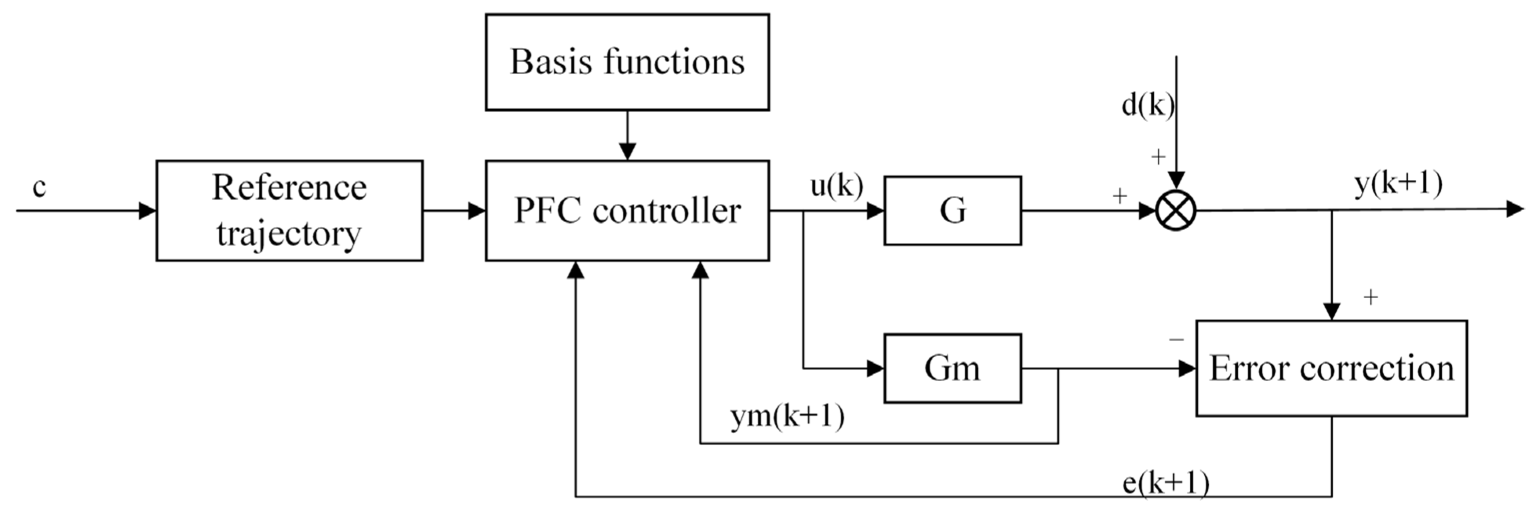
3.1. Predictive Functional Control (PFC) Algorithm

The predictive functional control algorithm belongs to the third generation of predictive control, which has three basic characteristics of general predictive control: predictive model, rolling optimization, and feedback correction [27]. The biggest feature of PFC is the structured control input; the control input at each moment is represented by the linear combination of the pre-selected basis function family, and then the linear weighting coefficient is calculated through online optimization, and then the current control input is calculated [28]. The structure diagram of the predictive functional controller is shown in Figure 2.

In Figure 2, $G$ is the controlled object, $G_m$ is the prediction model, $c$ is the set output value, $u\left(k\right)$ is the amount of control, $d\left(k\right)$ is the interference, $y\left(k+1\right)$ is the output of the actual system, $y_m\left(k+1\right)$ is the output of the prediction model, and $e\left(k+1\right)$ is the prediction error.

In predictive functional control, the control input is a linear combination of a set of basis functions $f_j\left(j=1,2,\cdots ,N\right)$ related to processing characteristics and tracking setpoints, namely:

$$u\left(k+i\right)={\displaystyle \sum _{j=1}^N{\mu }_j{f}_j\left(i\right)}\begin{array}{cc}& i=0,1,\cdots ,H-1\end{array}$$

(18)

where, N is the number of basis functions; ${\mu }_j$ is the linear combination coefficient; $H$ is the prediction optimization time-domain length.

Generally, the choice of basis function mainly depends on the set value and the nature of the controlled object, such as the step function, slope function, or parabola function. If the set value is constant or has a small change rate between controlled regions, select a basis function, that is, the step function. When the change rate of the set value is greater than a certain value in the controlled area, two basic functions, namely, the step function and the slope function, are selected.

The output $y_m\left(k\right)$ of the prediction model is composed of the model-free response $y_l\left(k\right)$ and the forced response $y_f\left(k\right)$, then the model forced response at the time $\left(k+i\right)$ is:

$$y_f\left(k+i\right)={\displaystyle \sum _{j=1}^N{\mu }_j}{g}_j\left(i\right)$$

(19)

where, $g_j\left(i\right)$ is the model output under the action of the basis function $f_j\left(i\right)$.

The model output at the time $\left(k+i\right)$ is:

$$y_m\left(k+i\right)=y_l\left(k+i\right)+y_f\left(k+i\right)$$

(20)

The model of the prediction functional takes the state space equation, and its discrete state space expression is:

$$\left\{\begin{array}{l}{X}_m\left(k\right)=A_m{X}_m\left(k\right)+B_{m}u\left(k\right)\hfill \\ y_m\left(k\right)=C_m{X}_m\left(k\right)\hfill \end{array}\right.$$

(21)

where, $X_m\in R^{n\times 1}$ is the state vector of the prediction model, $y_m\in R^{1\times 1}$ is the prediction output of the prediction model, $u\in R^{1\times 1}$ is the control input of the prediction model, $A_m\in R^{n\times n},B_m\in R^{n\times 1},C_m\in R^{1\times n}$ are the system matrices of the prediction model.

According to Equation (21), the expression of the model state at the time $\left(k+i\right)$ can be derived as:

$$\begin{array}{l}{X}_m\left(k+i\right)=A_m^i{X}_m\left(k\right)+A_m^{i-1}{B}_{m}u\left(k\right)+A_m^{i-2}{B}_{m}u\left(k-1\right)+\cdots \\ +A_m{B}_{m}u\left(k+i-2\right)+B_{m}u\left(k+i-1\right)\end{array}$$

(22)

According to Equations (18), (19), and (22), the output of the model at the time $\left(k+i\right)$ can be obtained by recursion as follows:

$$y_m\left(k+i\right)=C_m{A}_m^i{X}_m\left(k\right)+{\mu }^T\left(k\right)g_k\left(i\right)$$

(23)

where,

$$\left\{\begin{array}{l}\mu \left(k\right)={\left[{\mu }_1\left(k\right){\mu }_2\left(k\right)\cdots {\mu }_N\left(k\right)\right]}^T\hfill \\ g_k\left(i\right)=\left[g_{k1}\left(i\right)g_{k2}\left(i\right)\cdots g_{kN}\left(i\right)\right]\hfill \\ g_{kj}\left(i\right)=C_m{A}_m^{i-1}{B}_m{f}_j\left(0\right)+C_m{A}_m^{i-2}{B}_m{f}_j\left(1\right)+\cdots +C_m{B}_m{f}_j\left(i-1\right)\hfill \end{array}\right.$$

(24)

For a stable system, the first-order exponential form is generally chosen to describe the reference trajectory, namely:

$$y_r\left(k+i\right)=y_c\left(k+i\right)-{\beta }^i\left(y_c\left(k\right)-y\left(k\right)\right)\begin{array}{c}\hspace{1em}\hspace{1em}\hspace{1em}i=1,2,\cdots ,h-1\end{array}$$

(25)

where, $y_r\left(k+i\right)$ is the reference trajectory value at the sampling time of $\left(k+i\right)$, $y_c\left(k+i\right)$ is the quasi-tracking set value of the system at the sampling time of $\left(k+i\right)$, $y\left(k\right)$ is the actual output response value of the system at the sampling time of $k$. $\beta$ is the softening coefficient of the reference trajectory and satisfies $\beta =e^{-3T_s/T_r}$, $\beta \in \left(0,1\right)$. Where, $T_s$ is the sampling period and $T_r$ is the desired system closed-loop response time. $\beta$ is the rate at which the predicted output of the regulation system tracks the setpoint approach.

The optimized performance index of predictive functional control involves the future behavior of the system. The performance index can be used to obtain the control input. Generally, the size of the current and future control inputs of the controlled object can be determined based on the performance index. These control inputs will make the predictive model output of the controlled object follow the reference trajectory to achieve the ultimate goal of making the actual output of the system track the set value. The usual optimization criterion is to minimize the sum of squares of the reference trajectory at the optimization point and the prediction error output of the prediction process. The expression of the optimization objective function in this paper is shown in Equation (26).

$$J\left(k\right)=\min {\displaystyle \sum _{i=1}^H{\left[y\left(k+i\right)-y_r\left(k+i\right)\right]}^2}$$

(26)

where: $H$ refers to the predictive time-domain length, which mainly affects the stability and robustness of the control.

$$y\left(k+i\right)=y_m\left(k+i\right)+e\left(k+i\right)$$

(27)

where, $y\left(k+i\right)$ is the system output; $y_m\left(k+i\right)$ is the output of the generalized predictive model; $e\left(k+i\right)$ is a systematic error.

3.2. PID Control Algorithm

The controller with proportional, integral, and differential links is called the PID controller, which is the most widely used control law in the field of industrial process control. The continuous PID control equation is shown in Equation (28) [29].

$$u\left(t\right)=k_p\left[e\left(t\right)+\frac{1}{T_I}{\displaystyle \int e\left(t\right)dt+T_D\frac{de\left(t\right)}{dt}}\right]$$

(28)

where, $e\left(t\right)$ is the temperature deviation, $k_p$ is the scale factor, $T_I$ is the integration time, $T_D$ is the differential time.

Since the computer deals with digital quantities, Equation (28) is discretized, and the control law expression of digital PID is obtained as shown in Equation (29).

$$u\left(k\right)=k_{p}e\left(k\right)+k_i{\displaystyle \sum _{j=0}^{k}e\left(j\right)}+k_d\left[e\left(k\right)-e\left(k-1\right)\right]$$

(29)

where, $e\left(k\right)$ is the input temperature deviation value when the sampling time is $k$; $k_p$ is the scale factor; $k_i=k_p\frac{T}{T_I}$, $k_d=k_p\frac{T_D}{T}$, $T$ is the sampling period.

The incremental PID control algorithm is:

$$\Delta u(k)=k_p\Delta e\left(k\right)+k_{i}e\left(k\right)+k_d\left[\Delta e\left(k\right)-\Delta e\left(k-1\right)\right]$$

(30)

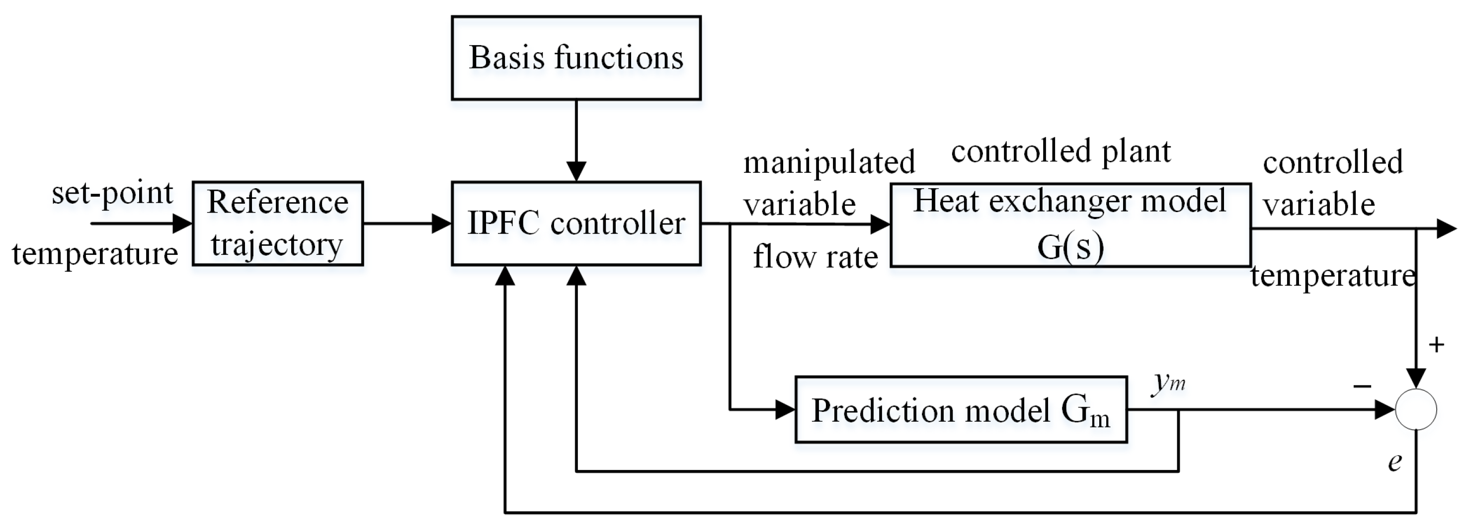
3.3. Improved PFC (IPFC) Control Algorithm

The predictive functional control algorithm has good tracking ability and strong robustness for time-delay system control. PID control has a strong anti-interference ability. To control the system better, the structural features of proportional, integral, and differential in the PID control algorithm are added to the optimal objective function of the PFC, so that the improved controller has the advantages of both predictive functional control and PID control.

From Equations (26) and (30), the PID-based PFC optimization function can be expressed as:

$$\begin{array}{l}J={\displaystyle \sum _{i=1}^H\left\{k_p\times {\left[\Delta e\left(k+i\right)\right]}^2+k_i\times {\left[e(k+i)\right]}^2+k_d\times {\left[{\Delta }^{2}e\left(k+i\right)\right]}^2\right\}}\\ +\beta {{\displaystyle \sum _{i=1}^{H-1}\left[\Delta u\left(k+i\right)\right]}}^2\end{array}$$

(31)

Make:

$$\left\{\begin{array}{l}e={\left[e\left(k+1\right)e\left(k+2\right)\cdots e\left(k+H\right)\right]}^T\hfill \\ \Delta e={\left[\Delta e\left(k+1\right)\Delta e\left(k+2\right)\cdots \Delta e\left(k+H\right)\right]}^T\hfill \\ {\Delta }^{2}e={\left[{\Delta }^{2}e\left(k+1\right){\Delta }^{2}e\left(k+2\right)\cdots {\Delta }^{2}e\left(k+H\right)\right]}^T\hfill \\ \Delta u={\left[\Delta u\left(k\right)\Delta u\left(k+1\right)\cdots \Delta u\left(k+H-1\right)\right]}^T\hfill \end{array}\right.$$

(32)

From Equation (27) to Equation (30), we can get:

$$\begin{array}{l}y\left(k+i\right)-y_r(k+i)={\mu }^T\left(k\right)g_k\left(i\right)+\\ \left\{\left(1-{\beta }^i\right)y\left(k\right)-y_c\left(k+i\right)+{\beta }^i{y}_c\left(k\right)+C_m\left(A_m^i-I\right)X_m\left(k\right)\right\}\end{array}$$

(33)

Make:

$$d\left(k+i\right)=\left\{\left(1-{\beta }^i\right)y\left(k\right)-y_c\left(k+i\right)+{\beta }^i{y}_c\left(k\right)+C_m\left(A_m^i-I\right)X_m\left(k\right)\right\}$$

(34)

So:

$$e\left(k+i\right)=y\left(k+i\right)-y_r\left(k+i\right)={\mu }^T\left(k\right)g_k\left(i\right)+d\left(k+i\right)$$

(35)

Make:

$$\left\{\begin{array}{c}{g}_k={\left[g_k\left(1\right)g_k\left(2\right)\cdots g_k\left(H\right)\right]}^T=\left[\begin{array}{cccc}{g}_{k1}\left(1\right)& g_{k1}\left(2\right)& \cdots & g_{k1}\left(H\right)\\ g_{k2}\left(1\right)& g_{k2}\left(2\right)& \cdots & g_{k2}\left(H\right)\\ ⋮& ⋮& ⋮& ⋮\\ g_{kN}\left(1\right)& g_{kN}\left(2\right)& \cdots & g_{kN}\left(H\right)\end{array}\right]\hfill \\ d=\left[\begin{array}{c}d\left(k+1\right)\\ d\left(k+2\right)\\ ⋮\\ d\left(k+H\right)\end{array}\right]\hfill \\ \Delta d=\left[\begin{array}{c}\Delta d\left(k+1\right)\\ \Delta d\left(k+2\right)\\ ⋮\\ \Delta d\left(k+H\right)\end{array}\right]=\left[\begin{array}{c}d\left(k+1\right)-d\left(k\right)\\ d\left(k+2\right)-d\left(k+1\right)\\ ⋮\\ d\left(k+H\right)-d\left(k+H-1\right)\end{array}\right]\hfill \\ {\Delta }^{\text{2}}d=\left[\begin{array}{c}{\Delta }^{2}d\left(k+1\right)\\ {\Delta }^{2}d\left(k+2\right)\\ ⋮\\ {\Delta }^{2}d\left(k+H\right)\end{array}\right]=\left[\begin{array}{c}\Delta d\left(k+1\right)-\Delta d\left(k\right)\\ \Delta d\left(k+2\right)-\Delta d\left(k+1\right)\\ ⋮\\ \Delta d\left(k+H\right)-\Delta d\left(k+H-1\right)\end{array}\right]\hfill \end{array}\right.$$

(36)

So there are:

$$\left\{\begin{array}{c}\begin{array}{l}e=\left[\begin{array}{c}e\left(k+1\right)\\ e\left(k+2\right)\\ ⋮\\ e\left(k+H\right)\end{array}\right]=\left[\begin{array}{cccc}{g}_{k1}\left(1\right)& g_{k2}\left(1\right)& \cdots & g_{kN}\left(1\right)\\ g_{k1}\left(2\right)& g_{k2}\left(2\right)& \cdots & g_{kN}\left(2\right)\\ ⋮& ⋮& ⋮& ⋮\\ g_{k1}\left(H\right)& g_{k2}\left(H\right)& \cdots & g_{kN}\left(H\right)\end{array}\right]\left[\begin{array}{c}{\mu }_1\left(k\right)\\ {\mu }_2\left(k\right)\\ ⋮\\ {\mu }_N\left(k\right)\end{array}\right]-\left[\begin{array}{c}d\left(k+1\right)\\ d\left(k+2\right)\\ ⋮\\ d\left(k+H\right)\end{array}\right]\\ \text{=}{g}_k^T\mu \left(k\right)-d\end{array}\hfill \\ \begin{array}{l}\Delta e=\left[\begin{array}{c}\Delta e\left(k+1\right)\\ \Delta e\left(k+2\right)\\ ⋮\\ \Delta e\left(k+H\right)\end{array}\right]=\left[\begin{array}{c}e\left(k+1\right)-e\left(k\right)\\ e\left(k+2\right)-e\left(k+1\right)\\ ⋮\\ e\left(k+H\right)-e\left(k+H-1\right)\end{array}\right]\\ =\Delta g_k^T\mu \left(k\right)-\Delta d\end{array}\hfill \\ \begin{array}{l}{\Delta }^{2}e=\left[\begin{array}{c}\Delta e^{\text{2}}\left(k+1\right)\\ \Delta e^{\text{2}}\left(k+2\right)\\ ⋮\\ \Delta e^{\text{2}}\left(k+H\right)\end{array}\right]\\ \text{=}{\Delta }^2{g}_K^T\mu \left(k\right)-{\Delta }^{2}de\end{array}\hfill \end{array}\right.$$

(37)

Vectors and matrices are introduced here for easy derivation:

$$\mu ={\mu }^T\left(k\right)$$

(38)

Introduce the shift operator, then:

$$\Delta \mu =\mu \left(k\right)-\mu \left(k-1\right)=\mu \left(k\right)-q^{-1}\mu \left(k\right)=\left(1-q^{-1}\right)\mu$$

(39)

The same can be said for:

$$\begin{array}{l}{\Delta }^2\mu =\Delta \mu \left(k\right)-\Delta \mu \left(k-1\right)\\ =\left[\mu \left(k\right)-\mu \left(k-1\right)\right]-\left[\mu \left(k-1\right)-\mu \left(k-2\right)\right]\\ =\mu \left(k\right)-\mu \left(k-1\right)-\mu \left(k-1\right)+\mu \left(k-2\right)\\ =\mu \left(k\right)-2q^{-1}\mu \left(k\right)+q^{-2}\mu \left(k\right)\\ =\left(1-2q^{-1}+q^{-2}\right)\mu \end{array}$$

(40)

$$\left\{\begin{array}{l}g=g_k\left(i\right)\hfill \\ \Delta g=\left(1-q^{-1}\right)g\hfill \\ {\Delta }^{2}g=\left(1-2q^{-1}+q^{-2}\right)g\hfill \end{array}\right.$$

(41)

$$\left\{\begin{array}{l}d=d\left(k+i\right)\hfill \\ \Delta d=\left(1-q^{-1}\right)d\hfill \\ {\Delta }^{2}d=\left(1-2q^{-1}+q^{-2}\right)d\hfill \end{array}\right.$$

(42)

$$\left\{\begin{array}{l}e=\mu g-d\hfill \\ \Delta e=\Delta \mu \Delta g-\Delta d\hfill \\ {\Delta }^{2}e={\Delta }^2\mu {\Delta }^{2}g-{\Delta }^{2}d\hfill \end{array}\right.$$

(43)

Converting Equation (31) into vector form, we can get:

$$J=k_i{e}^{T}e+k_p{\left(\Delta e\right)}^T\Delta e+k_d{\left({\Delta }^{2}e\right)}^T{\Delta }^{2}e+\beta {\left(\Delta u\right)}^T\Delta u$$

(44)

Because the value of $\beta {\left(\Delta u\right)}^T\Delta u$ is relatively small, and its existence is to make the input $u$ more accurate, and the main research in this paper is on the control effect, so the influence of this is not considered. To simplify the calculation, the objective function formula can be omitted as follows:

$$J=k_i{e}^{T}e+k_p{\left(\Delta e\right)}^T\Delta e+k_d{\left({\Delta }^{2}e\right)}^T{\Delta }^{2}e$$

(45)

By substituting Equation (43) into the above equation, we get:

$$\begin{array}{l}J=k_i{\left(\mu g-d\right)}^T\left(\mu g-d\right)+k_p{\left(\Delta \mu \Delta g-\Delta d\right)}^T\left(\Delta \mu \Delta g-\Delta d\right)\\ +k_d{\left({\Delta }^2\mu {\Delta }^{2}g-{\Delta }^{2}d\right)}^T\left({\Delta }^2\mu {\Delta }^{2}g-{\Delta }^{2}d\right)\\ =k_i\left(g^T{\mu }^T-d^T\right)\left(g\mu -d\right)+k_p\left(\Delta g^T\Delta {\mu }^T-\Delta d^T\right)\left(\Delta \mu \Delta g-\Delta d\right)\\ +k_d\left({\Delta }^2{g}^T{\Delta }^2{\mu }^T-{\Delta }^2{d}^T\right)\left({\Delta }^2\mu {\Delta }^{2}g-{\Delta }^{2}d\right)\\ \text{=}{k}_i\left(g^T{\mu }^T\mu g-g^T{\mu }^{T}d-d^T\mu g+d^{T}d\right)\\ +k_p\left(\Delta g^T\Delta {\mu }^T\Delta \mu \Delta g-\Delta g^T\Delta {\mu }^T\Delta d-\Delta d^T\Delta \mu \Delta g+\Delta d^T\Delta d\right)\\ +k_d\left({\Delta }^2{g}^T{\Delta }^2{\mu }^T{\Delta }^2\mu {\Delta }^{2}g-{\Delta }^2{g}^T{\Delta }^2{\mu }^T{\Delta }^{2}g-{\Delta }^2{d}^T{\Delta }^2\mu {\Delta }^{2}g+{\Delta }^2{d}^T{\Delta }^{2}d\right)\\ =k_i\left(g^T{\mu }^T\mu g-g^T{\mu }^{T}d-d^T\mu g+d^{T}d\right)\\ +k_p\left[\Delta g^T\left(1-q^{-1}\right){\mu }^T\left(1-q^{-1}\right)\mu \Delta g-\Delta g^T\left(1-q^{-1}\right){\mu }^T\Delta d-\Delta d^T\left(1-q^{-1}\right)\mu \Delta g+\Delta d^T\Delta d\right]\\ +k_d\left[\begin{array}{l}{\Delta }^2{g}^T\left(1-2q^{-1}+q^{-2}\right){\mu }^T\left(1-2q^{-1}+q^{-2}\right)\mu {\Delta }^{2}g-{\Delta }^2{g}^T\left(1-2q^{-1}+q^{-2}\right){\mu }^T{\Delta }^{2}d\\ -{\Delta }^2{d}^T\left(1-2q^{-1}+q^{-2}\right)\mu {\Delta }^{2}g+{\Delta }^2{d}^T{\Delta }^{2}d\end{array}\right]\end{array}$$

(46)

The purpose of objective function optimization is to obtain a set of optimal coefficients and then calculate the optimal control input so that $J$ obtains a minimum value. When $\mathit{\partial }J/\mathit{\partial }\mu =0$, the control input can be:

$$\begin{array}{l}{k}_i\left(g^{T}2\mu g-g^{T}d-d^{T}g\right)\\ +k_p\left[\Delta g^T\left(1-q^{-1}\right)\left(1-q^{-1}\right)2\mu \Delta g-\Delta g^T\left(1-q^{-1}\right)\Delta d-\Delta d^T\left(1-q^{-1}\right)\Delta g\right]\\ +k_d\left[\begin{array}{l}{\Delta }^2{g}^T\left(1-2q^{-1}+q^{-2}\right)\left(1-2q^{-1}+q^{-2}\right)2\mu {\Delta }^{2}g\\ -{\Delta }^2{g}^T\left(1-2q^{-1}+q^{-2}\right){\Delta }^{2}d-{\Delta }^2{d}^T\left(1-2q^{-1}+q^{-2}\right){\Delta }^{2}g\end{array}\right]=0\end{array}$$

(47)

The formula can be simplified as follows:

$$\begin{array}{l}2k_i{g}^T\mu g+2{\left(1-q^{-1}\right)}^4{k}_p{g}^T\mu g+2{\left(1-2q^{-1}+q^{-2}\right)}^4{k}_d{g}^T\mu g\\ =k_i\left(g^{T}d+d^{T}g\right)+k_p{\left(1-q^{-1}\right)}^3\left(g^{T}d+d^{T}g\right)+k_d{\left(1-2q^{-1}+q^{-2}\right)}^3\left(g^{T}d+d^{T}g\right)\end{array}$$

(48)

In this case, the linear weighting coefficient $\mu$ is:

$$\begin{array}{l}\mu =\frac{k_i\left(g^{T}d+d^{T}g\right)+k_p{\left(1-q^{-1}\right)}^3\left(g^{T}d+d^{T}g\right)+k_d{\left(1-2q^{-1}+q^{-2}\right)}^3\left(g^{T}d+d^{T}g\right)}{2k_i{g}^T\mathrm{g}+2{\left(1-q^{-1}\right)}^4{k}_p{g}^T\mathrm{g}+2{\left(1-2q^{-1}+q^{-2}\right)}^4{k}_d{g}^{T}g}\\ =\frac{\left[k_i+k_p{\left(1-q^{-1}\right)}^3+k_d{\left(1-2q^{-1}+q^{-2}\right)}^3\right]\left(g^{T}d+d^{T}g\right)}{2g^{T}g\left[k_i+{\left(1-q^{-1}\right)}^4{k}_p+{\left(1-2q^{-1}+q^{-2}\right)}^4{k}_d\right]}\end{array}$$

(49)

For the convenience of calculation, let:

$$k=\frac{\left[k_i+k_p{\left(1-q^{-1}\right)}^3+k_d{\left(1-2q^{-1}+q^{-2}\right)}^3\right]}{2\left[k_i+{\left(1-q^{-1}\right)}^4{k}_p+{\left(1-2q^{-1}+q^{-2}\right)}^4{k}_d\right]}$$

(50)

Then the linear weighting coefficient $\mu$ can be expressed as:

$$\mu =k\frac{\left(g^{T}d+d^{T}g\right)}{g^{T}g}$$

(51)

By substituting the linear weighting coefficient formula into the control equation, the control equation that will eventually act on the controlled object can be written as follows:

$$u\left(k+i\right)=f_k{}^T\left(0\right)\mu =f_k{}^T\left(0\right)k\frac{\left(g^{T}d+d^{T}g\right)}{g^{T}g}$$

(52)

where:

$$f_k^T\left(0\right)={\left[f_{k1}\left(0\right)f_{k2}\left(0\right)\cdots f_{kj}\left(0\right)\right]}^T$$

(53)

3.4. Control System Structure

The improved PFC controller proposed in this paper is applied to the outlet temperature control system of the heat exchanger, and its structure is shown in Figure 3.

The manipulated variable is the fluid flow rate $MV=G_2$, the controlled variable is the exchanger output temperature $CV=T_{1o}$. The heat exchanger model $G\left(s\right)$ in the figure is shown in Equation (14). The prediction model $G_m$ is chosen as $G_m\left(s\right)=\frac{1.9}{106s^2+26s+1}{e}^{-5.2s}$.

The set value is the step signal, and the unit step function is selected as the basis function. The control quantity of the IPFC controller at any given time $k$ can be obtained as:

$$\begin{array}{l}u\left(k+i\right)=f_k{}^T\left(0\right)\mu =1\times k\frac{\left(g^{T}d+d^{T}g\right)}{g^{T}g}\\ =\frac{\left[k_i+k_p{\left(1-q^{-1}\right)}^3+k_d{\left(1-2q^{-1}+q^{-2}\right)}^3\right]}{2\left[k_i+{\left(1-q^{-1}\right)}^4{k}_p+{\left(1-2q^{-1}+q^{-2}\right)}^4{k}_d\right]}\frac{\left(g^{T}d+d^{T}g\right)}{g^{T}g}\end{array}$$

(54)

At this time, we can control the output of the IPFC controller by adjusting the three parameters $k_p$, $k_i$, and $k_d$.

Meanwhile, in the IPFC control in this paper, to adjust signals more conveniently, constraint conditions are considered for IPFC, and the upper limit $u_{up}$ and lower limit $u_{low}$ are added to the calculated control variables [30]:

$$u_{low}\le u\left(k\right)\le u_{up}$$

(55)

Then, the restricted manipulation variable $u_{lim}\left(k\right)$is:

$$u_{\lim }\left(k\right)=\left\{\begin{array}{c}{u}_{up}\begin{array}{c}\hspace{1em}\hspace{1em}u\left(k\right)>u_{up}\end{array}\hfill \\ u\left(k\right)\begin{array}{c}\hspace{1em}\hspace{1em}\hspace{1em}{u}_{low}\le u\left(k\right)\le u_{up}\end{array}\hfill \\ u_{low}\begin{array}{c}\hspace{1em}\hspace{1em}u\left(k\right)<u_{low}\end{array}\hfill \end{array}\right.$$

(56)

At this point, the finite control variables will act as input signals to the model in the controller, as shown in Figure 4. The IPFC module and the limiting module constitute the IPFC controller, and the processing module refers to the heat exchanger system model. In the subsequent simulation in this paper, the limit of $u_{lim}\left(k\right)$ was between ±3.

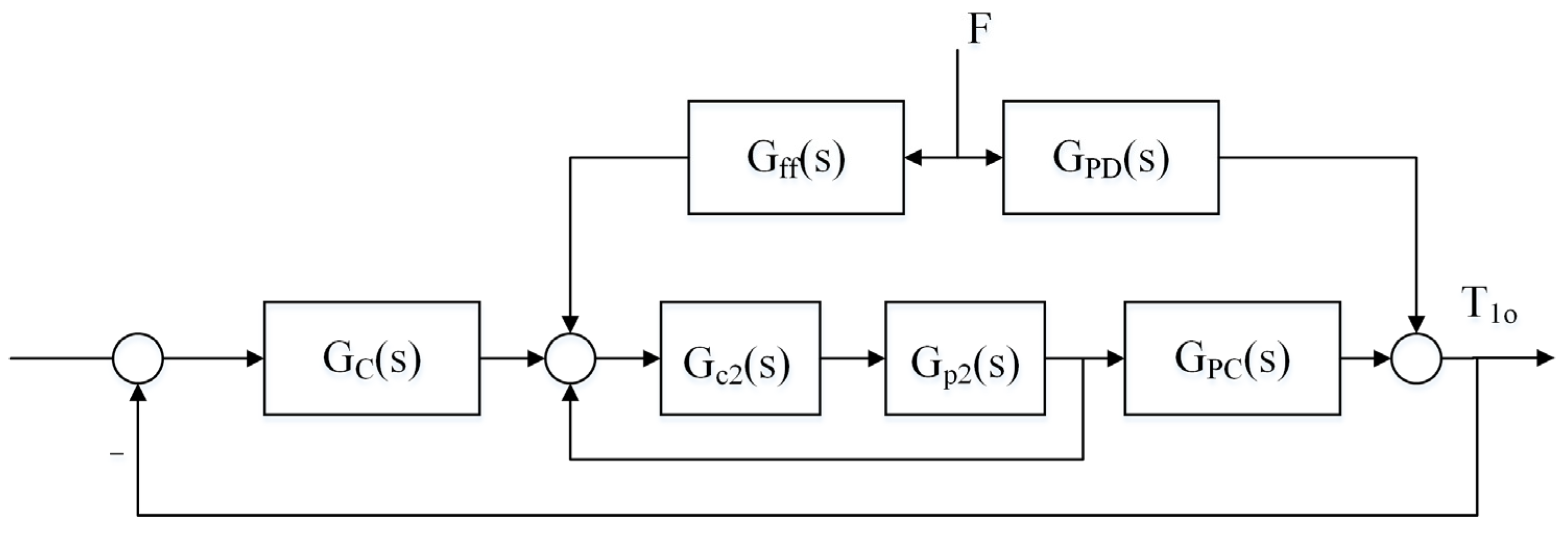
4. A Feedforward-Cascade Compound Control Scheme Based on IPFC

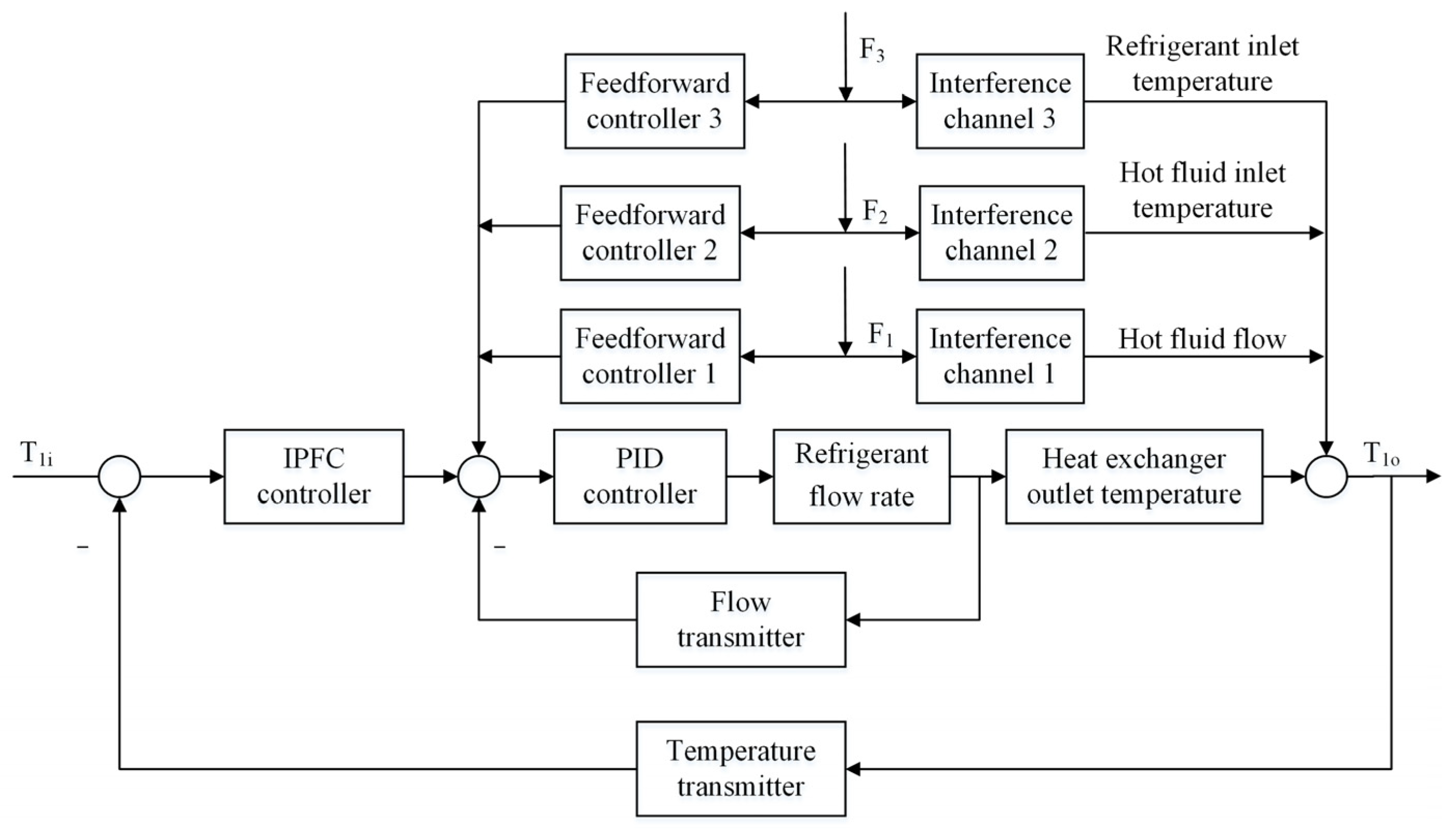
4.1. Feedforward-Cascade Compound Control System

Feedforward control, as an open-loop control system, is based on the measurable disturbance as the input of the controller, which then compensates for the deviation between the controlled variable and the set value and restores the controlled variable to a stable state according to the change in the disturbance quantity. A single feedforward is not very good at compensating interference, and there are many limitations. For example, a single feedforward control has no feedback link, and the compensation effect cannot be tested. As a result, when the feedforward fails to eliminate the deviation, the system cannot get the message for verification. In the actual industrial site, there are often many interference factors. If feedforward is used to compensate one by one, it is necessary to design multiple feedforward channels, which consumes money and power. Therefore, to solve these limitations, feedforward control and feedback control are generally combined [31].

For the heat exchanger outlet temperature control system, the common control scheme takes the refrigerant flow as the control variable to control the thermal fluid outlet temperature stability. Aiming at the typical feedforward feedback control system of the heat exchanger, its working principle is to superimpose the output value of the feedforward controller on the output value of the feedback controller and send it to the control valve together. This replaces the desired relationship between hot fluid flow and refrigerant flow with that between hot fluid flow and valve head pressure. To make the accuracy of feedforward compensation finer, a control valve with higher control quality is needed to meet the requirements of sensitivity, linearity, and minimal hysteresis, and the pressure difference before and after the control valve is required to remain unchanged. To solve the problem just mentioned, cascade control is adopted in the feedback loop, and refrigerant flow regulation is added in the secondary loop. The output effect of the feedforward controller is superimposed on that of the main loop controller as the given value of refrigerant flow regulation, which forms the feedforward-cascade compound control scheme.

The feedforward-cascade compound control system of the heat exchanger is shown in Figure 5 [32]. The simplified corresponding block diagram is shown in Figure 6 [33].

According to Figure 6, the transfer function of the system is listed as follows:

$$\frac{T_{1o}\left(s\right)}{F\left(s\right)}=\frac{G_{PD}\left(s\right)+G_{ff}\left(s\right)G_{\mathrm{p}2}^{\prime }\left(s\right)G_{PC}\left(s\right)}{1+G_c\left(s\right)G_{\mathrm{p}2}^{\prime }\left(s\right)G_{PC}\left(s\right)}$$

(57)

where, $G_{p2}^{\prime }\left(s\right)$ is the transfer function of the equivalent object of the secondary loop:

$$G_{\mathrm{p}2}^{\prime }\left(s\right)=\frac{G_{c2}\left(s\right)G_{p2}\left(s\right)}{1+G_{c2}\left(s\right)G_{p2}\left(s\right)}$$

(58)

According to the invariance condition:

$$F\left(s\right)\ne 0 \mathrm{and} T_{1o}\left(s\right)\equiv 0$$

(59)

The transfer function of $G_{ff}$ can be obtained by substituting it into Formula (57):

$$G_{ff}\left(s\right)=-\frac{G_{PD}\left(s\right)}{G_{\mathrm{p}2}^{\prime }\left(s\right)G_{PC}\left(s\right)}$$

(60)

4.2. Control Scheme

The heat exchanger studied in this paper has four input variables: refrigerant flow, refrigerant inlet temperature, hot fluid flow, and hot fluid inlet temperature; the refrigerant flow is a control variable, and the thermal fluid outlet temperature is a controlled variable; the other three variables are not controllable and can only exist as a disturbance. According to the characteristics of feedforward control, feedforward control is the preferred control scheme when there are large-scale and high-frequency disturbances in the system that can be measured but cannot be used as control variables. Therefore, this paper proposes a feedforward cascade compound control scheme based on IPFC. The feedforward control is used to compensate the three interference channels of hot fluid flow, hot fluid inlet temperature, and refrigerant inlet temperature, and the other small disturbances, such as pressure fluctuations, are corrected by feedback control.

In this paper, three feedforward channels are designed to compensate for and control the three disturbances, respectively. The thermal fluid flow is in interference channel 1, and the corresponding feedforward compensation is feedforward controller 1. The inlet temperature of hot fluid is interference channel 2, and the corresponding feedforward compensation is feedforward controller 2. The refrigerant inlet temperature is interference channel 3, and the corresponding feedforward compensation is feedforward controller 3. Meanwhile, the characteristics of feedback and cascade control systems are used to control other small disturbances.

The schematic diagram of the control scheme is shown in Figure 7.

5. Simulation Experiment and Result Analysis

5.1. Transfer Function of Feedforward Controller

According to the dynamic and static characteristics analysis and modeling of each channel of the heat exchanger in Section 2, the transfer function of the controlled object can be obtained as follows: $G_{PC}\left(s\right)=\frac{1.9}{105.7s^2+25.7s+1}{e}^{-5.14s}$; The transfer function of the main disturbance, namely the hot fluid flow to the outlet temperature channel, is: $G_{PD1}\left(s\right)=\frac{-1.35}{105.7s^2+25.7s+1}{e}^{-5.14s}$; The transfer function of the temperature channel at the inlet of the hot fluid is: $G_{PD2}\left(s\right)=\frac{0.464}{37.66s+1}$; The transfer function of the temperature channel at the refrigerant inlet is: $G_{PD3}\left(s\right)=\frac{0.536}{105.7s^2+25.7s+1}{e}^{-5.14s}$. In this paper, the transfer function of the secondary loop flow regulating valve is: $G_{p2}\left(s\right)=\frac{1}{s+1}$, PID controller parameter: $k_p=0.3, k_i=0.00001, k_d=0.1$, so: $G_{c2}\left(s\right)=\left(0.3+\frac{0.00001}{s}+0.1s\right)$.

Then, according to Equation (58), it can be obtained:

$$G_{\mathrm{p}2}^{\prime }\left(s\right)=\frac{G_{c2}\left(s\right)G_{p2}\left(s\right)}{1+G_{c2}\left(s\right)G_{p2}\left(s\right)}=\frac{0.1s^2+0.3s+0.00001}{1.1s^2+1.3s+0.00001}$$

(61)

The transfer function of the hot fluid flow to feedforward controller 1 of the outlet temperature channel is:

$$G_{ff1}\left(s\right)=-\frac{G_{PD1}\left(s\right)}{G_{\mathrm{p}2}^{\prime }\left(s\right)G_{PC}\left(s\right)}=\frac{0.781s^2+0.923s+0.0000071}{0.1s^2+0.3s+0.00001}$$

(62)

Since the constant term in the numerator and denominator is too small, it is omitted here; the above formula can then be simplified as follows:

$$G_{ff1}\left(s\right)=\frac{0.781s+0.923}{0.1s+0.3}$$

(63)

Similarly, the transfer function of feedforward controller 2 from the inlet temperature of the hot fluid to the outlet temperature channel is:

$$G_{ff2}\left(s\right)=-\frac{G_{PD2}\left(s\right)}{G_{\mathrm{p}2}^{\prime }\left(s\right)G_{PC}\left(s\right)}\approx -0.244\frac{165.68s^2+34.51s+1.3}{3.766s^2+11.398s+0.3}$$

(64)

The transfer function of feedforward controller 3 from the refrigerant inlet temperature to the outlet temperature channel is:

$$G_{ff3}\left(s\right)=-\frac{G_{PD3}\left(s\right)}{G_{\mathrm{p}2}^{\prime }\left(s\right)G_{PC}\left(s\right)}=-\frac{0.3102s+0.3666}{0.1s+0.3}$$

(65)

According to the structural analysis of the feedforward control system, we can know that the control law of the feedforward controller is determined by the disturbance channel and the control channel in general. The heat exchanger and this kind of object contain aperiodic properties and over-damping properties, so they can be used to express the first- or second-order capacity lag, which according to the characteristics of the control system, can be connected with a pure lag to approximate. At this point:

$$G_{PD}\left(s\right)=\frac{K_2}{T_{2}s+1}{e}^{-{\tau }_{2}s}$$

(66)

$$G_{PC}\left(s\right)=\frac{K_1}{T_{1}s+1}{e}^{-{\tau }_{1}s}$$

(67)

Then:

$$G_{ff}\left(s\right)=-\frac{G_{PD}\left(s\right)}{G_{PC}\left(s\right)}=-K_f\frac{T_{1}s+1}{T_{2}s+1}{e}^{-{\tau }_{f}s}$$

(68)

where, $K_f=\frac{K_2}{K_1}$, is the static feedforward amplification coefficient; ${\tau }_f={\tau }_2-{\tau }_1$.

When there is little difference between ${\tau }_1$ and ${\tau }_2$, Equation (68) can be simplified as follows:

$$G_{ff}\left(s\right)=-K_f\frac{T_{1}s+1}{T_{2}s+1}$$

(69)

At this point, according to Equation (69), we can simplify the transfer function of feedforward controller 1 in this paper, namely Formula (70), into:

$$G_{ff1}\left(s\right)=\frac{0.781s+0.923}{0.1s+0.3}=-(-3.07)\frac{0.847s+1}{0.33s+1}$$

(70)

where: $K_f=-3.07$, $T_1=0.847$, $T_2=0.33$.

Similarly, the transfer function of feedforward controller 3 is simplified as follows:

$$G_{ff3}\left(s\right)=-\frac{0.3102s+0.3666}{0.1s+0.3}=-1.22\frac{0.847s+1}{0.33s+1}$$

(71)

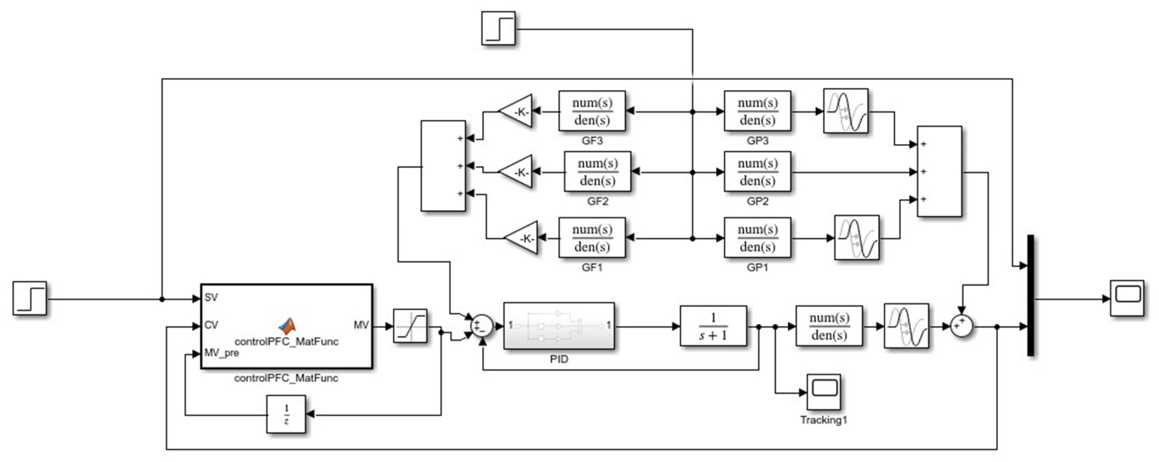
5.2. Simulation Experiment

According to the feedforward-cascade compound control system scheme based on IPFC proposed in this paper, the simulation model is built in Simulink, as shown in Figure 8. The proposed compound control system based on the IPFC main controller (IPFC-PID) and the compound control system based on the PID main controller (PID-PID) are simulated and compared under the same conditions to observe the control effect.

For the compound control system based on a PID main controller, the transfer function of the controlled object and the disturbance channel is consistent with that of the feedforward cascade compound control system based on IPFC. When the cascade control system reaches a stable state, the PID controller parameter in the inner loop is: $k_p=0.1, k_i=0.007, k_d=0.01$, so: $G_{c2}\left(s\right)=\left(0.1+\frac{0.007}{s}+0.01s\right)$. PID controller parameters in the main loop are $P=7, I=0.03, D=3$. The transfer function of the feedforward controller of each channel can be obtained by substituting into the formula in the previous section: $G_{ff1}\left(s\right)=\frac{0.7171s^2+0.781s+0.00497}{0.01s^2+0.1s+0.007}$, $G_{ff2}\left(s\right)=-0.1\frac{65.874s^2+13.58s+0.51}{0.715s^2+7.174s+0.19}$, $G_{ff3}\left(s\right)=-0.282\frac{1.01s^2+1.1s+0.007}{0.01s^2+0.1s+0.007}$.

In the IPFC-PID algorithm, according to the principle of the control algorithm, the PID controller is used for inner loop control and the IPFC is used for outer loop control. The controlled objects of the inner loop and main loop are combined as the generalized controlled objects of IPFC. The system identification is simplified through fitting. The corresponding first-order addition hysteresis model is: $G\left(s\right)=\frac{0.77}{21.825s+1}{e}^{-15.355s}$, This model is used as the prediction model for the external loop IPFC controller. The initialization parameters are as follows: First in the inner loop PID controller: $k_p=0.3, k_i=0.00001, k_d=0.1$. In the main loop IPFC controller, the sampling period: $t_s=0.1s$. System closed loop response time: $t_r=0.6s$. Predictive optimization time domain: $H=30$. $k_p=10,k_i=10,k_d=1$.

(1)

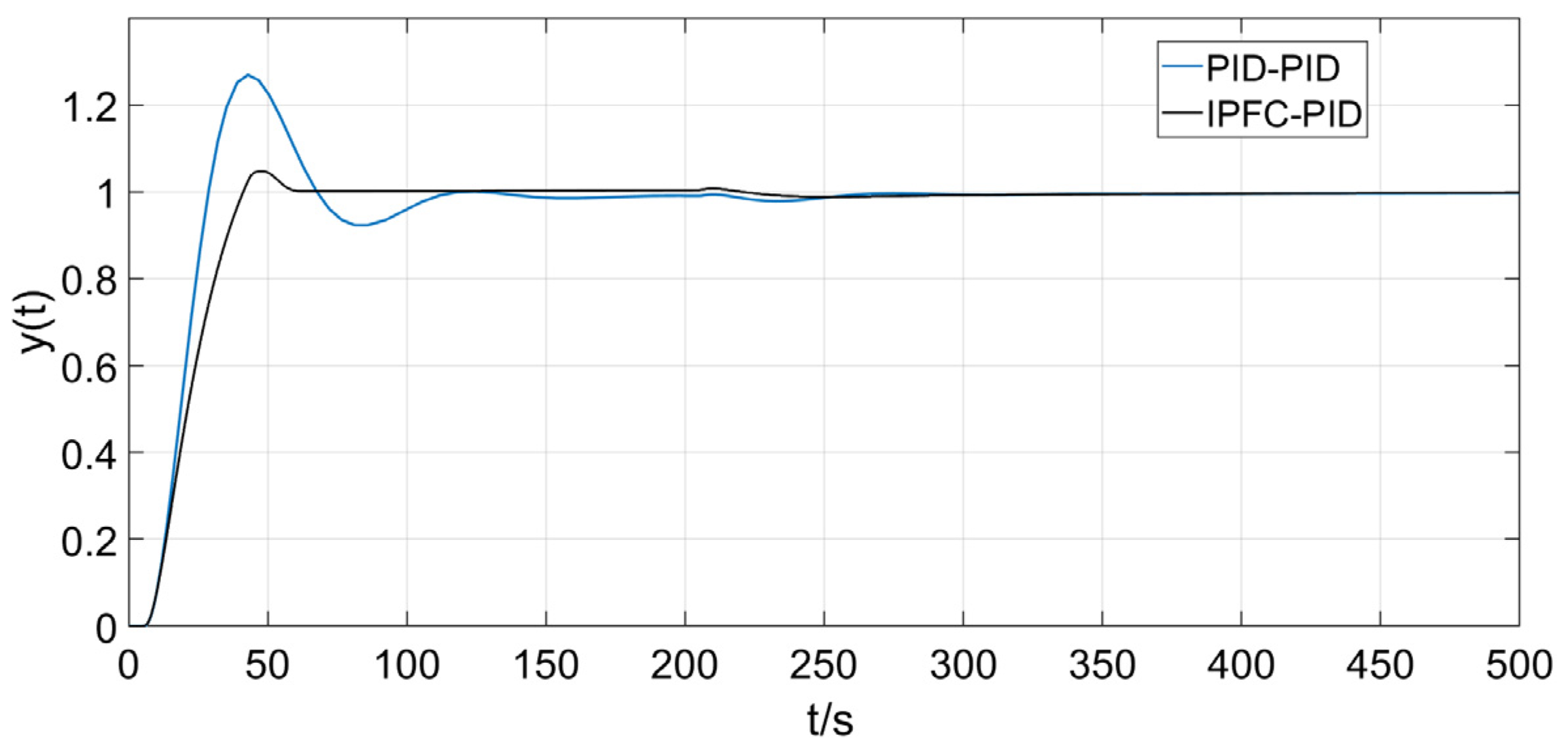
Model matching

Because there may be a variety of burst factors at the industrial site, the most representative disturbance can be decomposed into multiple sets of step signals when the system is running, and usually, the step input has the greatest impact on the system. To effectively reduce the influence of multi-source interference on the heat exchanger system, the output of the system is analyzed, and the step disturbance is given as the disturbance signal in this paper.

After the system reached a stable state, step disturbance signals were added to the three channels, respectively, and the inhibition effect of the feedforward control scheme on disturbance was observed.

When only the flow of hot fluid fluctuates, the other two channels are disconnected. At this time, a 0.5 step disturbance is added to interference channel 1 when the simulation reaches 200 s. The simulation effect is shown in Figure 9.

When only the temperature of the hot fluid inlet fluctuates, the other two channels are disconnected. At this time, a 0.5 step disturbance is added to interference channel 2 when the simulation reaches 200 s. The simulation effect is shown in Figure 10.

When only the temperature of the refrigerant inlet fluctuates, the other two channels are disconnected. At this time, a step disturbance of 0.5 is added to interference channel 3 when the simulation reaches 200 s. The simulation effect is shown in Figure 11.

When a disturbance occurs in the three channels of hot fluid flow, hot fluid inlet temperature, and refrigerant flow, the output of the control system in the simulation is 200 s, as shown in Figure 12.

From Figure 9 to Figure 12, dynamic performance indexes of the control effect of the two control schemes when each model is matched can be obtained, and their index values are shown in

Table 3. Dynamic performance index.

Item	Rise Time (s)	Adjustment Time (s)	Overshoot (%)
PID-PID	26.30	105.40	26.90
IPFC-PID	36.00	54.60	4.60

.

From Figure 9 to Figure 12, it can be seen that when interference occurs in each interference channel, the feedforward control scheme proposed in this paper can always well compensate for the influence of disturbance on the system, and the interference can be suppressed in advance by feedforward control before the deviation of heat exchanger outlet temperature is caused. At the same time, when the input of three kinds of heat exchangers is disturbed at the same time, the control scheme responds quickly and can make the system restore stability quickly; the adjustment time is short, and the overshoot is small, showing the control scheme’s better adaptive ability. Because part of the parameter calculation is omitted when calculating the feedforward controller parameters of the thermal fluid outlet temperature to the controlled object channel, the system deviation is more obvious when the thermal fluid outlet temperature is interfered with than the other two channels, but under the auxiliary control of IPFC as the main controller, the system can still be restored to stability. In addition, it can be seen from the data in Table 3 that the control effect of the IPFC controller proposed in this paper is stronger than that of the PID controller. Compared with the PID controller, the adjustment time and overshoot of the proposed control scheme are significantly reduced, and the adjustment time is shortened by 50.8 s. The overshoot is reduced by 22.3%, and the control effect is good.

(2)

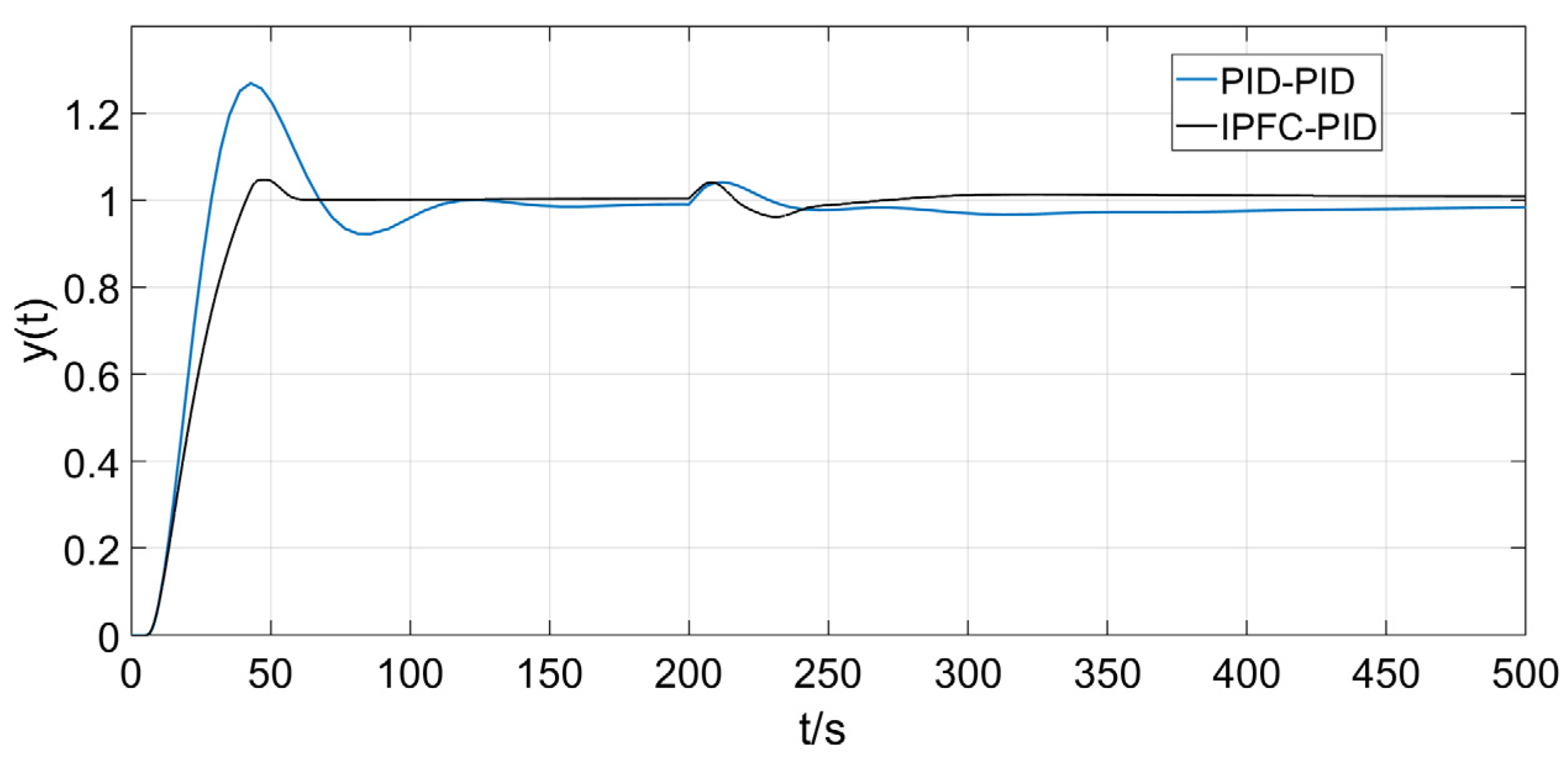
Interference channel model mismatch

In the actual industrial field, the controlled object may be affected by different situations, and the situation of model mismatch occurs. To test the control ability of the scheme under the condition of model mismatch, the adjustment parameters of the master and slave controllers and the parameters of the feedforward controller remain unchanged; the parameters of the disturbance channel are changed; and the same disturbance as the model matching is added to observe the control effect.

In this case, the transfer function of the main disturbance, namely the hot fluid flow to the outlet temperature channel, is: $G_{PD1}\left(s\right)=\frac{-1.35}{107s^2+23s+1}{e}^{-5.14s}$, The transfer function of the inlet temperature of hot fluid to the outlet temperature channel is: $G_{PD2}\left(s\right)=\frac{0.6}{40s+1}$, The transfer function of the temperature channel at the refrigerant inlet is: $G_{PD3}\left(s\right)=\frac{0.5}{112s^2+27s+1}{e}^{-5.14s}$.

When the model is mismatched, only when the hot fluid flow fluctuates, a step disturbance of 0.5 is added to interference channel 1. The simulation effect is shown in Figure 13.

When the model is mismatched, only the temperature of the hot fluid inlet fluctuates. At this time, a 0.5 step disturbance is added to interference channel 2 when the simulation reaches 200 s, and the simulation effect is shown in Figure 14.

When the model is mismatched, only when the temperature of the refrigerant inlet fluctuates, a 0.5 step disturbance is added to interference channel 3 when the simulation reaches 200 s, and the simulation effect is shown in Figure 15.

When the model is mismatched, the three channels of hot fluid flow, hot fluid inlet temperature, and refrigerant flow are disturbed, and the output of the control system in the simulation to 200 s is shown in Figure 16.

In the case of model mismatch, it can be seen from the simulation diagram that, compared with the scheme with PID as the main controller, the proposed control scheme can better suppress the disturbance and produce little fluctuation. For the feedforward controllers with more accurate parameter settings, such as feedforward controller 1 and feedforward controller 3, the interference can be corrected or minimized before it enters the process. The disturbance does not affect the controlled object.

(3)

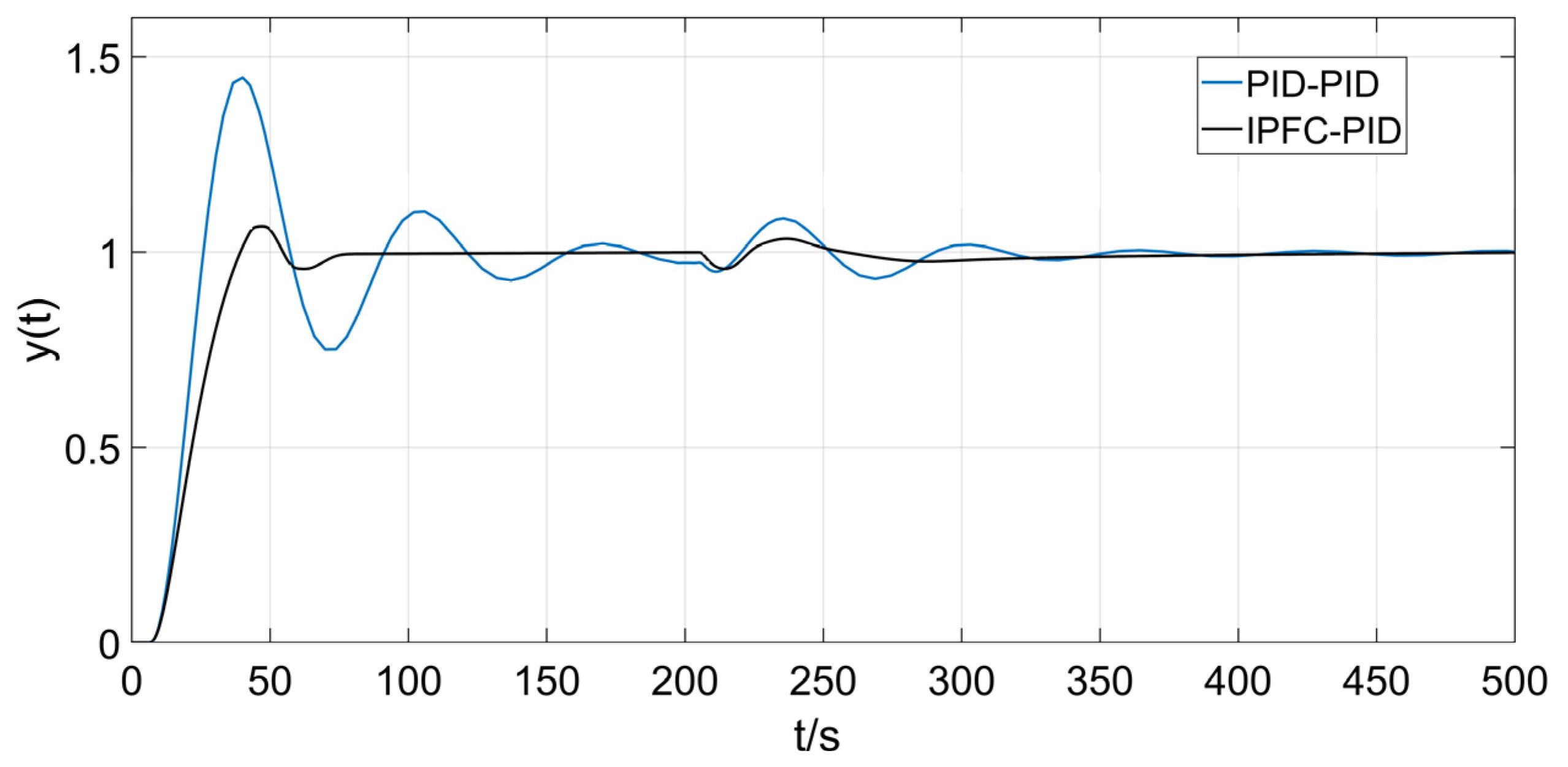
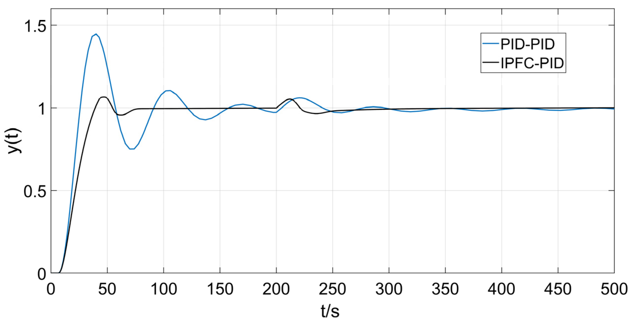
Controlled object model mismatch

To demonstrate the control effect of the control scheme when modeling errors occur in the transfer function of the controlled object, the adjustment parameters of the master and slave controllers, the parameters of the feedforward controller, and the parameters of the disturbance channel are kept unchanged, and the mathematical model parameters of the controlled object are changed and set as:$G_{PC}\left(s\right)=\frac{2}{110.8s^2+20.56s+1}{e}^{-6.168s}$. The same disturbance as the model matching was added to observe the control effect.

When the model is mismatched, the step disturbance of 0.5 is added to interference channel 1 only when the hot fluid flow is disturbed. The simulation effect is shown in Figure 17.

When the model is mismatched, the step disturbance of 0.5 is added to interference channel 2 only when the thermal fluid inlet temperature is disturbed. The simulation effect is shown in Figure 18.

When the model is mismatched, a step disturbance of 0.5 is added to interference channel 3 only when the refrigerant inlet temperature is disturbed. The simulation effect is shown in Figure 19.

In the case of model mismatch, when the three interference channels of hot fluid flow, hot fluid inlet temperature, and refrigerant flow are disturbed, the output of the control system is shown in Figure 20.

When a model mismatch occurs in the transfer function of the controlled object, the corresponding simulation curves under different types of disturbance are shown in Figure 17, Figure 18, Figure 19 and Figure 20. The corresponding dynamic performance indicators are shown in

Table 4. Dynamic performance index under model mismatch.

Item	Rise Time (s)	Adjustment Time (s)	Overshoot (%)
PID-PID	24.40	153.10	45.20
IPFC-PID	34.24	70.93	6.60

.

It can be seen from the simulation diagram and dynamic performance indicators that when the mathematical model of the controlled object is mismatched due to modeling errors or other disturbances, the feedforward cascade compound control scheme based on the PID controller has a poor control effect, large overshooting, a long adjustment time, and a poor suppression effect on the disturbance of the three groups of hot fluid flow, hot fluid inlet temperature, and refrigerant inlet temperature. However, the feedforward cascade compound control scheme based on IPFC proposed in this paper has a good control effect, a short regulation time, a small overkill, and a strong inhibition effect against the disturbance of the three groups of input variables, which can make the system quickly restore to a stable state.

6. Discussion

The heat exchanger is an important piece of equipment for energy exchange in the chemical industry. To improve the energy utilization efficiency of the system and maintain its efficient and stable operation of the system, it is of great significance to study the outlet temperature control system of the heat exchanger. PID control is one of the earliest development control strategies. Due to its simple algorithm, strong robustness, and high reliability, it is widely used in industrial process control. However, because in the process of actual industrial production, the controlled objects often have the characteristics of non-linearity and time-degeneration, it is difficult to establish a precise mathematical model. The conventional PID controller cannot achieve the ideal control effect. Predictive control is a kind of advanced control technology based on a model that combines the actual demands of industry to the maximum extent. It adopts the strategies of prediction models, rolling optimization, and feedback correction, and is suitable for an industrial process where it is not easy to establish accurate mathematical models and is complicated. Therefore, this paper combines the predictive function control algorithm with the PID control algorithm. The improved controller inherits the advantages of both and has a better control effect on the outlet temperature system of the heat exchanger. For the reason that the heat exchanger temperature control system has four input variables, the commonly used control scheme is to control the refrigerant flow to adjust the temperature of the thermal fluid outlet, and the other three input variables are generally determined by the output of the upper-level system, which can be measured and uncontrollable, generally as a disturbance. Therefore, this paper proposes a feedforward cascade compound control scheme based on IPFC that provides feedforward control for three groups of important external disturbances to offset the influence of disturbances on the control system.

In the process control of the chemical industry, light industry, and other industries, most of the controlled objects have the characteristics of large lag, nonlinear, and large inertia, such as temperature, liquid level, flow rate, and other systems. The improved PFC control proposed in this paper has a good control effect for large lag and nonlinear systems and is suitable for similar industrial control systems.

The control scheme proposed in this paper also has some limitations.

(1)

The adjustment parameters of the improved predictive function control algorithm proposed in this paper need to be selected within a certain range so that the control system can be well controlled. For example, when using the particle swarm optimization algorithm, setting the search range of three parameters of $k_p,k_i$ and $k_d$ between [0, 50] can obtain a better control effect than between [0, 100]. How to further adjust the IPFC control algorithm is the next problem to be studied.

(2)

In this paper, the transfer function of the controlled object is obtained based on the theoretical analysis of the dynamic and static characteristics of the heat exchanger, and the transfer function of each interference channel is solved through the characteristic analysis. The controlled object is not tested and verified on the actual industrial site, so it may be different from the actual heat exchanger model, and the feedforward controller design needs to be further modified. This will be improved in future studies.

(3)

In the feedforward control scheme, this paper gives three feedforward controllers for the three main measurable uncontrollable interference compensations, but in the actual industrial process, the feedforward channel will increase enterprise investment costs and maintenance workload, so in the heat exchanger external disturbance situation, how to target all kinds of disturbance suppression and save investment and workload. Further research will also be needed.

7. Conclusions

This paper takes the heat exchanger outlet temperature control system as the control object. Aiming at the problems of large delay, nonlinearity, and multiple interferences, a feedforward cascade compound control system based on IPFC is proposed. Through the analysis of the simulation results, the following conclusions are drawn.

(1)

In this paper, the predictive functional control algorithm and PID control algorithm are combined, and the incremental PID control algorithm is used to improve the optimization objective function of the predictive functional control algorithm. By predicting the future output value of the controlled system and optimizing the control parameters of the controlled object, the analytical solution to the control quantity is obtained. The IPFC control algorithm has the structural characteristics of proportion, integration, and differentiation and has the advantages of strong robustness of the predictive functional control algorithm and good anti-interference of the PID control algorithm;

(2)

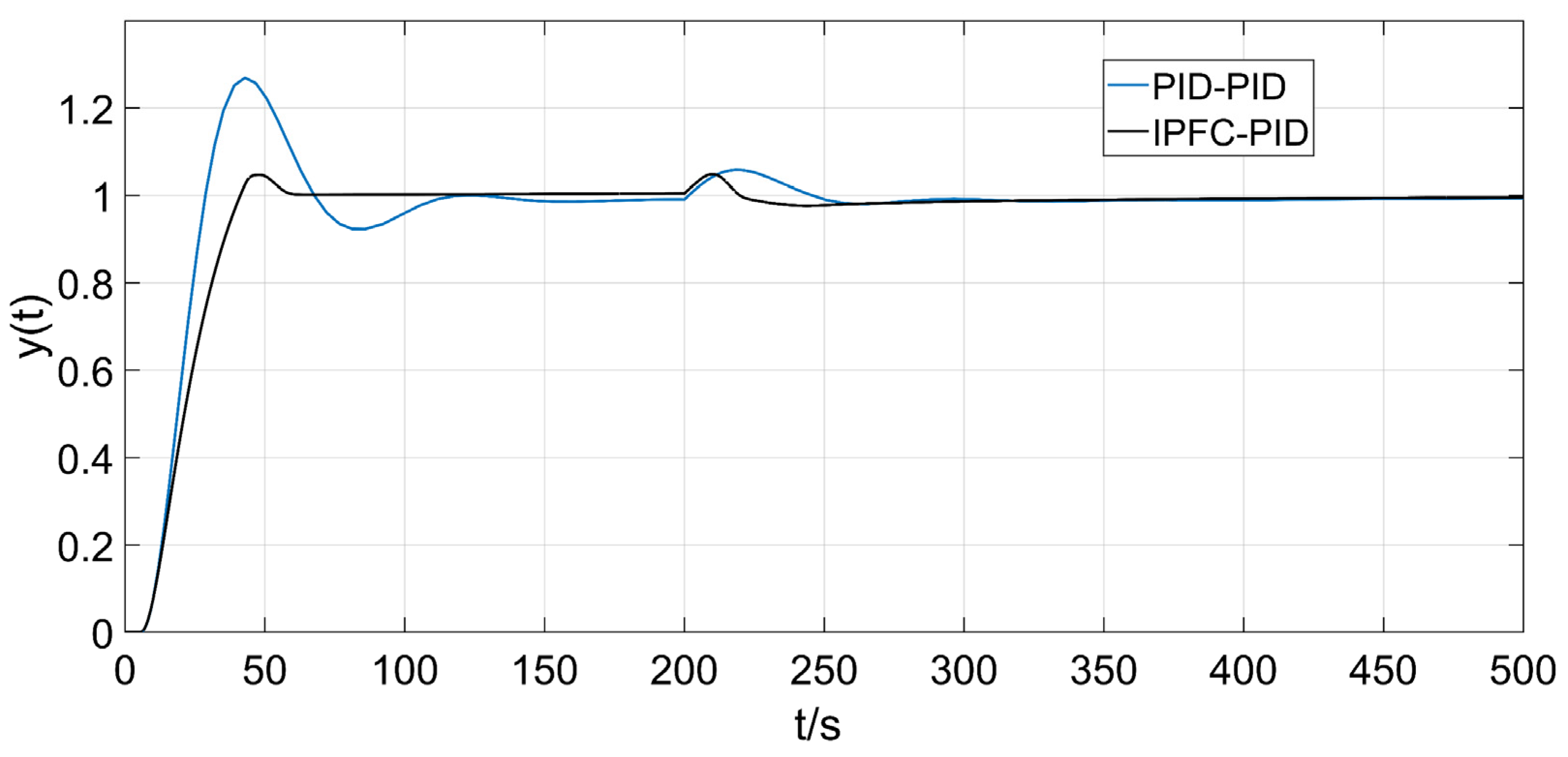
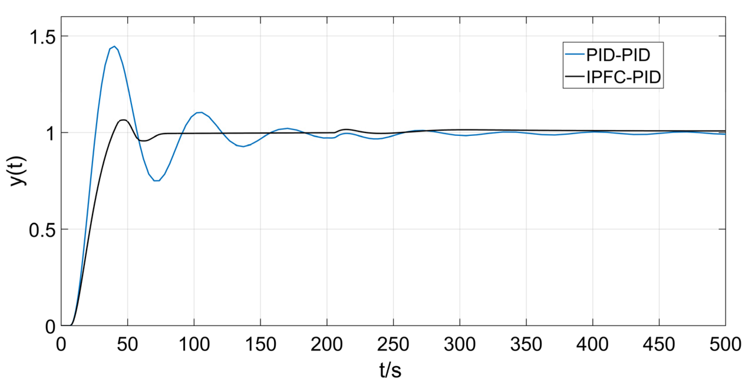
Compared with the feedforward cascade composite control scheme with PID as the main controller, before adding disturbance, it can be seen from the simulation comparison diagram that the control scheme proposed in this paper has a smaller overshot and adjustment time, which also confirms the effectiveness of the improved control algorithm proposed in this paper;

(3)

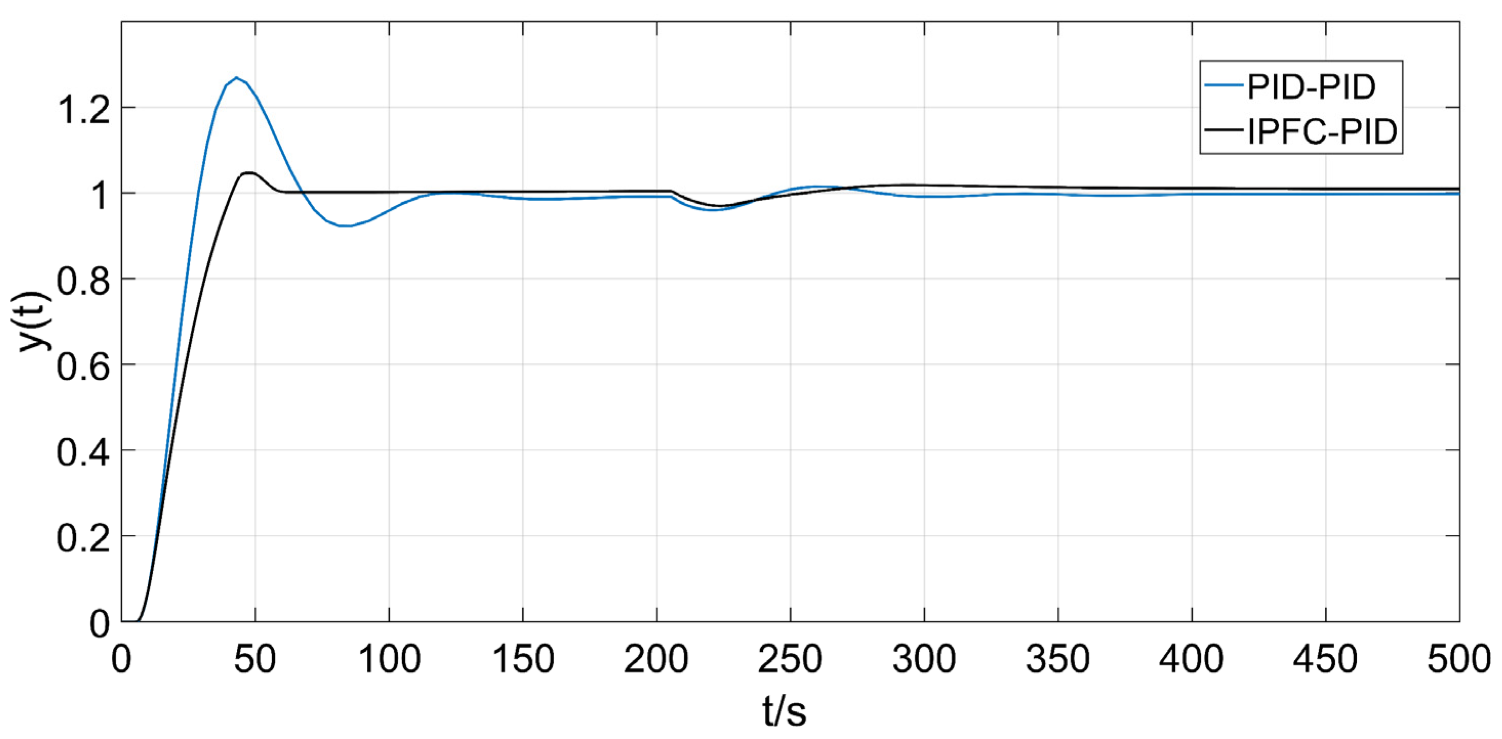
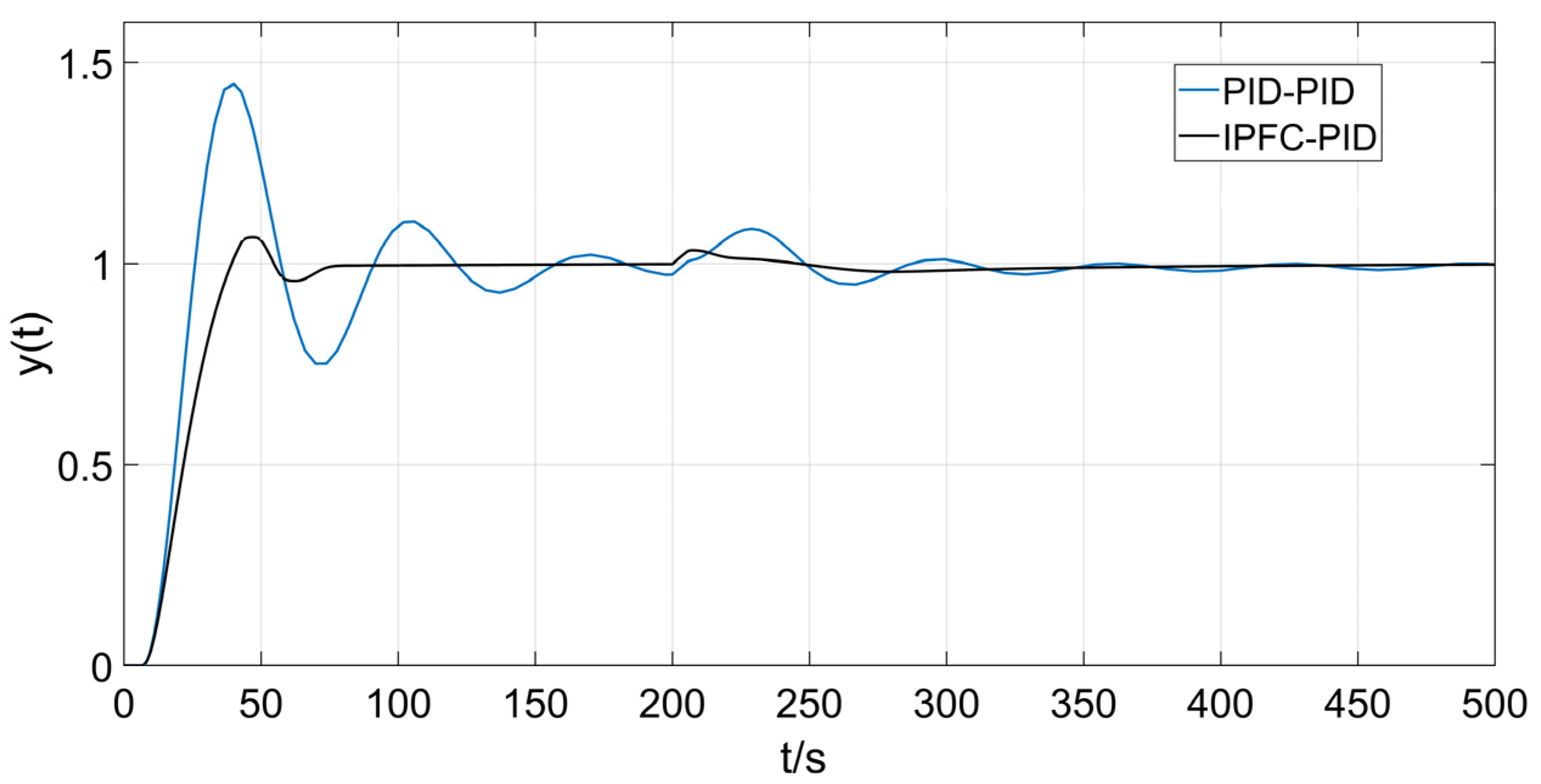
In the case of model matching and model mismatch, simulation is made for the three interference channels acting separately and simultaneously. Through the analysis of simulation comparison curves, it can be concluded that the feedforward cascade compound control system based on IPFC proposed in this paper has strong disturbance suppression ability and can correct or minimize the interference before it enters the process. The disturbance does not affect the controlled object.

References

- Wang, B.; Klemeš, J.J.; Li, N.; Zeng, M.; Varbanov, P.S.; Liang, Y. Heat exchanger network retrofit with heat exchanger and material type selection: A review and a novel method. Renew. Sustain. Energy Rev. 2020, 138, 110479. [Google Scholar] [CrossRef]
- Soave, N.; Barolo, M. On the Effectiveness of Heat-Exchanger Bypass Control. Processes 2021, 9, 244. [Google Scholar] [CrossRef]
- Huang, P.; Copertaro, B.; Zhang, X.; Shen, J.; Löfgren, I.; Rönnelid, M.; Fahlen, J.; Andersson, D.; Svanfeldt, M. A review of data centers as prosumers in district energy systems: Renewable energy integration and waste heat reuse for district heating. Appl. Energy 2019, 258, 114109. [Google Scholar] [CrossRef]
- Klemeš, J.J.; Kravanja, Z. Forty years of Heat Integration: Pinch Analysis (PA) and Mathematical Programming (MP). Curr. Opin. Chem. Eng. 2013, 2, 461–474. [Google Scholar] [CrossRef]
- Dulau, M.; Karoly, M.; Dulau, T.M. Fluid temperature control using heat exchanger. Procedia Manuf. 2018, 22, 498–505. [Google Scholar] [CrossRef]
- Ramadan, M.; Khaled, M.; ElHage, H.; Harambat, F.; Peerhossaini, H. Effect of air temperature non-uniformity on water-air heat exchanger thermal performance—Toward innovative control approach for energy consumption reduction. Appl. Energy 2016, 173, 481–493. [Google Scholar] [CrossRef]
- Jin, H.Z.; Gu, Y.; Ou, G.F. Corrosion risk analysis of tube-and-shell heat exchangers and design of outlet temperature control system. Pet. Sci. 2021, 18, 1219–1229. [Google Scholar] [CrossRef]
- Dong, Z.; Li, B.; Li, J.; Jiang, D.; Guo, Z.; Huang, X.; Zhang, Z. Passivity based control of heat exchanger networks with application to nuclear heating. Energy 2021, 223, 120107. [Google Scholar] [CrossRef]
- Yuan, Z.; Chen, B.; Sin, G.; Gani, R. State-of-the-art and progress in the optimization-based simultaneous design and control for chemical process. AIChE J. 2012, 58, 1640–1659. [Google Scholar] [CrossRef]
- Laszczyk, P. Simplified modeling of liquid-liquid heat exchangers for use in control systems. Appl. Therm. Eng. 2017, 119, 140–155. [Google Scholar] [CrossRef]
- Vrancic, D.; Oliveira, P.M.; Bistak, P.; Huba, M. Model-Free VRFT-Based Tuning Method for PID Controllers. Mathematics 2023, 11, 715. [Google Scholar] [CrossRef]
- Toyota, D.; Nakano, K.; Ochi, K.; Kinoshita, T.; Wakitani, S.; Yamamoto, T. Database-driven practical online adjustment of PID parameters. IEEJ Trans. Electr. Electron. Eng. 2022, 17, 705–712. [Google Scholar] [CrossRef]
- Wang, J.; Wu, X.C.; Li, Q.; Zhao, J. First Order Plus Dead Time Model Approximation and Proportional-Integral-Derivative Controllers Tuning for Multi-Volume Process. J. Nanoelectron. Optoelectron. 2022, 17, 794–808. [Google Scholar] [CrossRef]
- Salavati, S.; Grigoriadis, K.; Franchek, M. An explicit robust stability condition for uncertain time-varying first-order plus dead-time systems. ISA Trans. 2022, 126, 171–179. [Google Scholar] [CrossRef]
- Huba, M.; Vrancic, D. Tuning of PID Control for the Double Integrator Plus Dead Time Model by Modified Real Dominant Pole and Performance Portrait Methods. Mathematics 2022, 10, 971. [Google Scholar] [CrossRef]
- Huba, M.; Oliveira, P.M.; Bistak, P.; Vrancic, D.; Zakova, K. A Set of Active Disturbance Rejection Controllers Based on Integrator Plus Dead-Time Models. Appl. Sci. 2021, 11, 1671. [Google Scholar] [CrossRef]
- Nauman, M.; Shireen, W.; Hussain, A. Model-Free Predictive Control and Its Applications. Energies 2022, 15, 5131. [Google Scholar] [CrossRef]
- Vasičkaninová, A.; Bakošová, M. Control of a heat exchanger using neural network predictive controller combined with auxiliary fuzzy controller. Appl. Therm. Eng. 2015, 89, 1046–1053. [Google Scholar] [CrossRef]
- Czeczot, J.; Laszczyk, P.; Metzger, M. Local balance-based adaptive control in the heat distribution system—Practical validation. Appl. Therm. Eng. 2010, 30, 879–891. [Google Scholar] [CrossRef] [Green Version]
- Bakošová, M.; Oravec, J. Robust model predictive control for heat exchanger network. Appl. Therm. Eng. 2014, 73, 924–930. [Google Scholar] [CrossRef]
- Carvalho, C.B.; Carvalho, E.P.; Ravagnani, M.A.S.S. Implementation of a neural network MPC for heat exchanger network temperature control. Braz. J. Chem. Eng. 2020, 37, 729–744. [Google Scholar] [CrossRef]
- Oravec, J.; Bakosova, M.; Trafczynski, M.; Vasickaninova, A.; Meszaros, A.; Markowski, M. Robust model predictive control and PID control of shell-and-tube heat exchangers. Energy 2018, 159, 1–10. [Google Scholar] [CrossRef]
- Wu, S.; Hou, P.; Zou, H.B. An improved constrained predictive functional control for industrial processes: A chamber pressure process study. Meas. Control. 2020, 53, 833–840. [Google Scholar] [CrossRef]
- Vasičkaninová, A.; Bakošová, M.; Mészáros, A.; Klemeš, J.J. Neural network predictive control of a heat exchanger. Appl. Therm. Eng. 2011, 31, 2094–2100. [Google Scholar] [CrossRef] [Green Version]
- Sun, H.C.; Weng, W.Q.; Wei, J. Process Control Systems and Engineering, 3rd ed.; Chemical Industry Press: Beijing, China, 2010; pp. 176–180. (In Chinese) [Google Scholar]
- Liang, Y.L.; He, Y.Y. Simulation research on the grid connected generation system of solar thermal power generation. Therm. Sci. 2020, 24, 3239–3248. [Google Scholar] [CrossRef] [Green Version]
- Richalet, J.; O’Donovan, D. Predictive Functional Control: Principles and Industrial Applications, 1st ed.; Springer: London, UK, 2009; pp. 11–68. [Google Scholar]
- Wang, Y.Z.; Jin, Q.B.; Zhang, R.D. Improved fuzzy PID controller design using predictive functional control structure. ISA Trans. 2017, 71, 354–363. [Google Scholar] [CrossRef]
- Razvarz, S.; Vargas-Jarillo, C.; Jafari, R.; Gegov, A. Flow control of fluid in pipelines using PID controller. IEEE Access 2019, 7, 25673–25680. [Google Scholar] [CrossRef]
- Haber, R.; Bars, R.; Schmitz, U. Predictive Control in Process Engineering: From the Basics to the Applications, 1st ed.; Wiley-VCH: Weinheim, Germany, 2011; pp. 454–457. [Google Scholar]
- Liu, L.; Tian, S.; Xue, D.; Zhang, T.; Chen, Y. Industrial feedforward control technology: A review. J. Intell. Manuf. 2018, 30, 2819–2833. [Google Scholar] [CrossRef]
- Luyben, W.L. Comparison of additive and multiplicative feedforward control. J. Process Control 2022, 111, 1–7. [Google Scholar] [CrossRef]
- Nandong, J. A unified design for feedback-feedforward control system to improve regulatory control performance. Int. J. Control. Autom. Syst. 2015, 13, 91–98. [Google Scholar] [CrossRef]