Article

Prediction of Structural Damage Trends Based on the Integration of LSTM and SVR

School of Energy and Electrical Engineering, Chang’an University, Xi’an 710018, China
Appl. Sci. 2023, 13(12), 7135; https://doi.org/10.3390/app13127135
Submission received: 19 April 2023 / Revised: 6 June 2023 / Accepted: 9 June 2023 / Published: 14 June 2023

Abstract

:
Currently, accidents in civil engineering buildings occur frequently, resulting in significant economic damage and a large number of casualties. Therefore, it is particularly important to predict the trend of early damage to building structures. Early structural damages are difficult to correctly identify, and obtaining the required accuracy using a single traditional time-series prediction method is difficult. In this study, we propose a novel method based on the integration of support vector regression (SVR) and long short-term memory (LSTM) networks to predict structural damage trends. First, the acceleration vibration signal of the structure is decomposed using the variational mode decomposition (VMD) method, and the decomposed components are transformed with Hilbert transform to obtain the instantaneous frequency. Then, the instantaneous frequency is input into the LSTM–SVR integrated model for damage trend prediction. The results indicate that the VMD method effectively eliminates modal aliasing and decomposes various intrinsic components of the signal. Compared with individual LSTM and SVR models, the integration model has a higher prediction accuracy for small samples in a chaotic time series that is 6.56%, 2.56%, and 3.7%, respectively. The standard deviation of the absolute percentage error (SDAPE) values of the three operating conditions under the integrated method decreased 0.0994, 0.0869, and 0.0921, which improved the stability of prediction. The mean absolute percentage error (MAPE) of the integration method is an order of magnitude higher than that of the LSTM model.

1. Introduction

Large-scale equipment and structures are increasingly common among individual lives and in production processes. Issues, including corrosion aging, deformation, and damage, occur when such structures are subject to environmental erosion and various loads over long service periods. These problems affect the health of the structures to varying extents. In serious cases, such issues can lead to the fracture and collapse of the structure, threatening the safety of lives and property as well as destabilizing the development of the social economy [1,2]. It is thus necessary to implement maintenance measures at an early stage of damage instead of dealing with an accident after the damage occurs. The prediction of structural damage is one of the key measures to achieve early damage diagnosis and prediction [3,4].
However, the vibration signals of most engineering structures are relatively complex and exhibit characteristics such as nonlinearity and nonstationarity [5]. Using appropriate signal processing techniques to extract damage information when structural damage occurs is a key issue that needs to be addressed in structural health state prediction [6]. Although the wavelet transform proposed in the literature [7] has the characteristic of multi-resolution, it requires artificial selection of wavelet bases and lacks self-adaptability. Although empirical mode decomposition (EMD) in the literature [8] solves the problem of wavelet transform’s lack of self-adaptability, it still has some problems, such as modal aliasing, significant endpoint effects, and lack of a complete theoretical basis. Variational mode decomposition (VMD) [9] has a mature theoretical foundation. By decomposing signals into fixed-scale component signals, it can effectively solve the problem of modal aliasing with relatively weak endpoint effects. Wu Jiahui used VMD to decompose the power load series into subsequences with limited bandwidth, improving the prediction accuracy of power load [10]. Zhang Yagang et al. used VMD to decompose the wind speed into several IMF components that fluctuate around the central frequency, helping to restore its fluctuation characteristics during the prediction process [11].
The prediction of early structural damages requires appropriate time-series prediction methods. At present, there are many time-series prediction methods, such as the least squares support vector machine [12], auto-regressive integral moving average model (ARIMA) [13], artificial neural network [14,15], and deep learning model [16,17]. However, many current models have certain limitations in prediction research. For example, the traditional BP neural network is difficult to deal with long-term and complex problems, and its generalization ability is weak; the ARMA prediction model is easier to deal with stationary time series than non-stationary time series. Although the improved ARIMA model based on ARMA is suitable for the prediction of non-stationary time series, it is difficult to select the lag order in the model training period, and it is difficult to obtain the optimal value of the lag order. In the training process of the echo state network, the problem of local extremum is easy to appear, which affects the prediction effect of the model.
Long short-term memory (LSTM) networks have become a popular research model in the framework of the recurrent neural network (RNN) and even deep learning and have received extensive attention [18]. To date, LSTM has been widely used in machine health monitoring [19], the prediction of bearing life [20], remaining useful life [21], watershed pollutant flux [22], short-term wind power [23], temperature [24], car suspension health, lithium battery, and other fields. Fang et al. [25] implemented a loss function to iteratively refine and enhance the accuracy and robustness of traffic flow prediction based on Δ f r e e -LSTM; a large number of experiments on four benchmark datasets show that Δ f r e e -LSTM is superior to both canonical and nonparametric models. Lyu et al. [26] used Lebesgue sampling parallel state fusion LSTM (LS–PSF–LSTM) to predict a lithium-ion battery early-cycle stage RUL; the experiments demonstrated the effectiveness of the proposed method. Li et al. [27] proposed a CNN–LSTM deep-learning framework to consider the spatial–temporal correlations together with the extrinsic features for flight delay prediction. Remarkably, their methodology achieved an accuracy of 92.39%, thereby demonstrating its tremendous potential. Wu et al. [28] coupled LSTM to principal component analysis (PCA) and moving average (MA), respectively, and proposed that the coupling prediction model is better. Luo et al. [29] proposed a method that combined a multi-Gaussian fitting feature extraction method with an LSTM-based damage identification method to develop a health monitoring system with available vibration signals, which can significantly reduce computation time in the condition of achieving great prediction accuracy. With the continuous exploration of long-term and short-term memory networks by scholars and experts, more and more researchers put forward the innovation of the LSTM network model and training methods and are committed to improving the training accuracy and convergence speed of the model. Although LSTM has a strong fitting effect on long-term time-series prediction, it displays shortcomings in predictions with low sample data, and the prediction effect is not satisfactory. The support vector regression (SVR) learning algorithm is based on the principle of structural risk minimization with excellent small sample prediction performance. This method has been successfully applied in numerous prediction fields and provides unique advantages. Li et al. [30] presents a comprehensive prediction model that combines time-series decomposition, the least square method, sparrow search algorithm (SSA), and support vector regression (SVR). The effectiveness of this model was evaluated using monitoring data from E13–E14 and E17–E18 joints, opening–closing deformation, of an immersed tunnel in the Hong Kong–Zhuhai–Macao Bridge. Yu et al. [31] proposed a non-intrusive load decomposition method based on CNN + SVR substation, which can provide load composition information of different degrees of fine grain and can better understand the power information of the industry and users of the substation. Li et al. [32] analyzed different algorithms (BPNN, SVR, RF, LSTM, LSTM–SVR) to perform multivariate non-Gaussian wind pressure conditional simulation with spatial interpolation prediction, and their prediction performance measures (MAPE, RMSE, R) are compared. The results indicate that the combined algorithm (LSTM–SVR) can utilize a small amount of data to realize the multivariate non-Gaussian conditional simulation with spatial interpolation prediction more accurately. Pan et al. [33] presented a hybrid prediction model based on ARIMA and SVR, and the experimental results showed that the mixed model had high prediction accuracy and could accurately describe the complex change trend of the time series of the number of borrowers.
Although LSTM–SVR has been widely used in various fields and has achieved great achievements, there is little research in the field of structural damage monitoring. In this sense, we must find a high-precision and relatively practical prediction method according to the rules and characteristics of structural vibration state changes. In this paper, the VMD decomposition method and the LSTM–SVR integrated model are combined and applied to structural damage prediction, ultimately achieving an improvement in the overall algorithm prediction performance. It is of great significance to predict the damage trend of structures when there is less engineering vibration data in the future.

2. Theoretical Basis for Structural Health Damage Trend Prediction

2.1. Variational Mode Decomposition (VMD)

The theory of variational mode decomposition (VMD) [9] is a new non-stationary, nonlinear signal processing method proposed by Konstantin Dragomiretskiy in 2014. If the signal is decomposed into modal components, the constrained variational model is as follows:
min { u i } , { w i } { i t [ ( [ t ] + j π t ) u i ( t ) ] e j w i t 2 2 }
where u i is the function set of each modal component, and w i is the central frequency set of each component. In Equation (1), a quadratic penalty factor α and a Lagrange multiplier λ are introduced to convert them into unconstrained variational problems. The optimal solution of Equation (2) is obtained using the alternating direction multiplier algorithm.
L ( { u i , { w i , λ } ) = α i t [ ( δ ( t ) + j π t ) u i ( t ) ] e j w i t 2 2     + y i u i ( t ) 2 2     + λ ( t ) , y i = 1 i u i ( t )
where L { } represents the Lagrange function, and y represents the original signal.

2.2. Long Short-Term Memory (LSTM) Networks

LSTM is a special type of RNN network incorporating memory modules on top of a hidden RNN layer. An LSTM repeating module chain schematic diagram is shown in Figure 1 [34,35]. The multiplication calculation allows the LSTM memory block to store and access information over a long period of time, thereby relieving the problem of gradient disappearance. The LSTM model is more sensitive to long-term information learning because the information easily flows along with the cell without information loss. The input, forget, and output gates control how much new input flows into the CEC unit, store the information in the unit, and then output the unit streams to the remaining networks.
LSTM utilizes the following equation to iteratively calculate network mapping from input sequence X to output sequence Y, from t = 1 to t = T, which is similar to the RNN calculation. The initial c 0 = 0 and h 0 = 0:
i t = σ ( W i x t + U i h t 1 + b i )
f t = σ ( W f x t + U f h t 1 + b f )
o t = σ ( W o x t + U o h t 1 + b o )
C ˜ t = tanh ( W c x t + U c h t 1 + b c )
C t = f t C t 1 + i t C ˜ t
h t = o t tanh ( C t )
σ = 1 1 + e x
where W i , W f , and W o represent the weight matrix of the input, forget, and output gates, respectively. The hidden layer weight matrix is characterized by U i , U f , and U o , while b i , b f , and b o represent the corresponding gate structure bias matrix, respectively. σ is the nonlinear activation function, which is a logistic sigmoid; i t , f t , o t , and c t are the input, forget, and output gates and unit state vector at time t, respectively, which have the same size as the unit output vector h t . The element-wise multiplication of the two vectors is represented by ⊗.

2.3. Support Vector Regression (SVR)

SVR is a prediction model based on the principle of structural risk minimization with a good learning ability for small samples [36]. SVR uses a kernel function to map input variables into high-dimensional space, thereby transforming low-dimensional nonlinear problems into linear regression in high-dimensional space [37] and then predicting the data trend. The insensitive function SVR (ε-SVR) is introduced below.
For certain training samples ( x i , y i ) , x R d , y i R , and i = 1 , , n . The goal of SVR linear regression is to solve the following regression function:
f ( x ) = w x + b
where w R , b R , and ( w x ) are the dot product of w and x and meet the principle of structural risk minimization, namely:
Q ( w ) = 1 2 ( w w ) + C R e m p ( f )
where C refers to the regression error penalty factor, and R e m p ( f ) refers to the loss function.
Most of the main structural damages are caused by the stiffness decrease from the perspective of general structural damage characterization. When the structure has different degrees of stiffness damage, the system output acceleration is used to identify the gradual damage of the stiffness changes. The LSTM–SVR is used as the structure health prediction model in this paper. Since the instantaneous frequency can effectively reflect the health status changes in the structure [38], the model is divided into signal processing, data preprocessing, and LSTM–SVR network prediction.

3. Integrated Prediction Method Based on the LSTM–SVR Model

3.1. Dynamic Weight Coefficient of the Integration Model

The specific prediction framework of the integration method is shown in Figure 2. Herein, w is the dynamic weight, and Y(t) is the result of the respective prediction results of the LSTM model and SVR model added by multiplying weights [39].
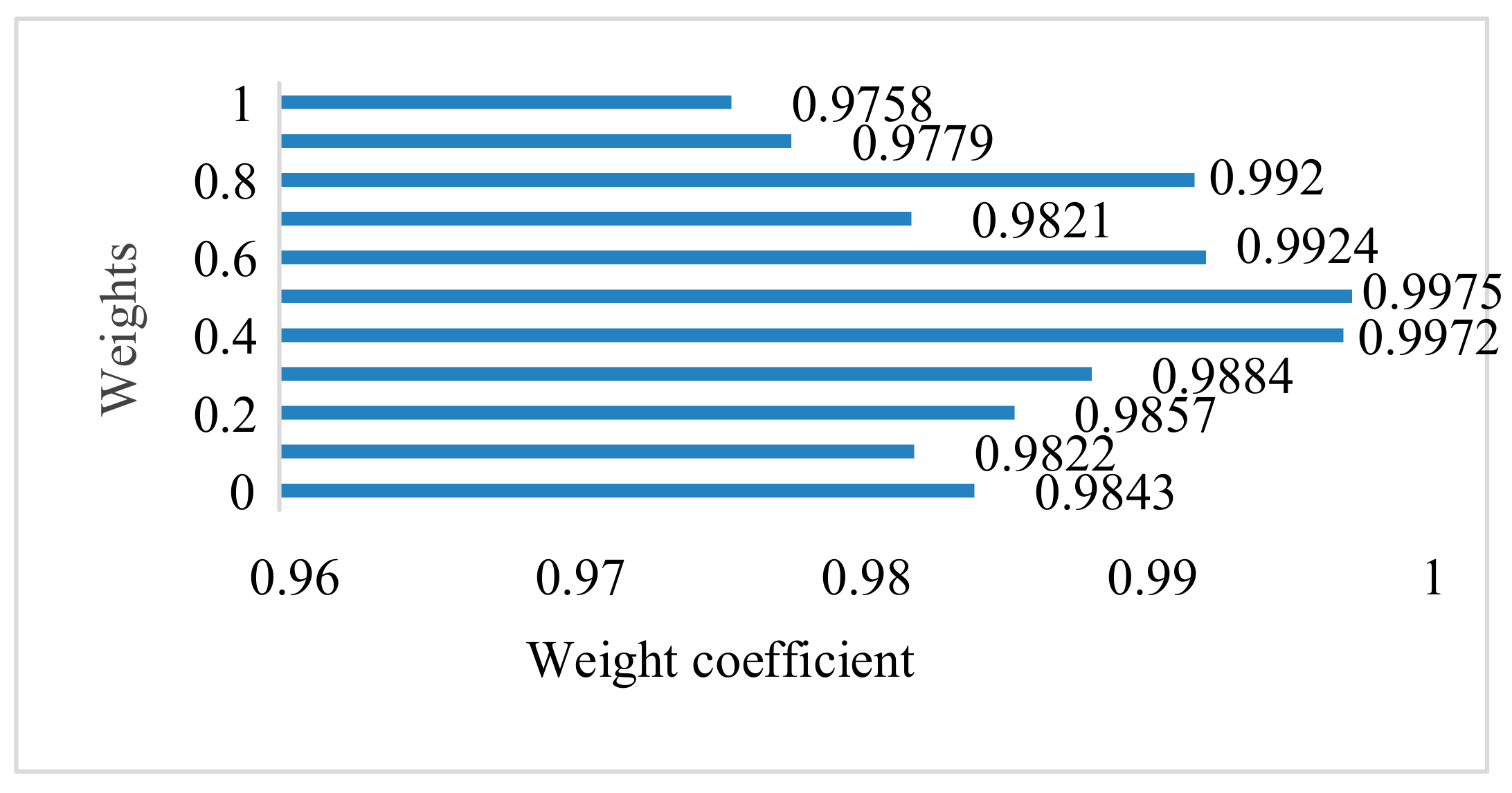
To achieve model integration, the optimized weight coefficient must be calculated. In this study, the weight coefficient takes a total of 11 values between 0 and 1.0. Figure 3 shows the process of integrating the two models. First, the weight coefficient is selected from 0.0 each time the prediction results of the two models are multiplied by their respective weights; then, the results of the two prediction models calculated by the weight coefficient are added together to obtain the weighted prediction results; finally, the first step is repeated until each weight has been calculated to obtain the corresponding predicted value.
Using the calculation shown in Figure 3, 11 sets of weight coefficients and corresponding prediction data as well as the determination coefficient R2 corresponding to the integration method are obtained. We display the obtained R2 in the manner shown in Figure 4. After comparing the R2 of each group, the weight corresponding to the prediction data group with the largest R2 is selected as the final coefficient of the prediction model of the integrated method in this paper.
Figure 4 shows that, when the weight coefficient is 0.5, the correlation between the fitting result of the fusion method and the actual value is the largest; that is, the integrated model has the highest prediction accuracy at this time. Thus, w = 0.5 is selected as the weight coefficient of the integrated prediction method.

3.2. Data Preprocessing

In order to facilitate analysis, improve training speed, and avoid the impact of dimensional differences between various data on the network model, it is necessary to standardize the data vector using the Z-score method based on various time series data [40] and normalize the input data vector into a standardized sequence with a mean value of 0 and a standard deviation of 1. The standardized expression is as follows:
x i = x i x ¯ i σ i
In the formula, x i represents the input data, x ¯ i represents the mean value of the data, and σ i is the standard deviation of the data.

3.3. Algorithm Evaluation Indicators

There are many indicators for evaluating prediction performance, and these quantifiable indicators can better reflect the pros and cons of prediction results. In this paper, root mean square error (RMSE), mean absolute percentage error (MAPE), standard deviation of absolute percentage error (SDAPE), coefficient of determination (R2), and refined Willmott index (RWI) are used as evaluation indicators for prediction effectiveness [41,42]:
(1)
Root mean square error:
R M S E = i = 1 N ( y i y i ) 2 N
(2)
Mean absolute percentage error:
M A P E = 1 N i = 1 N y i y i y i × 100 %
(3)
Standard deviation of absolute percentage error:
S D A P E = 1 N i = 1 N y i y i y i M A P E 2
(4)
Determination coefficient:
R 2 = i = 1 N ( y i y ¯ ) 2 i = 1 N ( y i y i ) 2 i = 1 N ( y i y ¯ ) 2
(5)
Refined Willmott index:
R W I = 1 i = 1 N y i y i 2 i = 1 N y i y ¯
where N represents the predicted data length, and y i and y i are the true value and the predicted value, respectively. The average absolute percentage error between y i and y i is represented by the RMSE, which reflects the average deviation between the true and predicted values. The value of RMSE is generally greater than or equal to 0, and when RMSE = 0, the prediction accuracy reaches the highest. The closer the MAPE is to 0 and the closer y i is to y i , the better is the prediction performance. The smaller the SDAPE value, the more robust is the prediction. The value of the R 2 is between 0 and 1 and is equal to 1 when there is no error. The RWI is between 0 and 1; a value of 1 means that the estimate exactly matches the actual value, and 0 means that the estimated value does not match the actual value at all. The above three indicators are used as the evaluation basis for the prediction performance of the model.

3.4. Verification and Analysis of the Integration Model

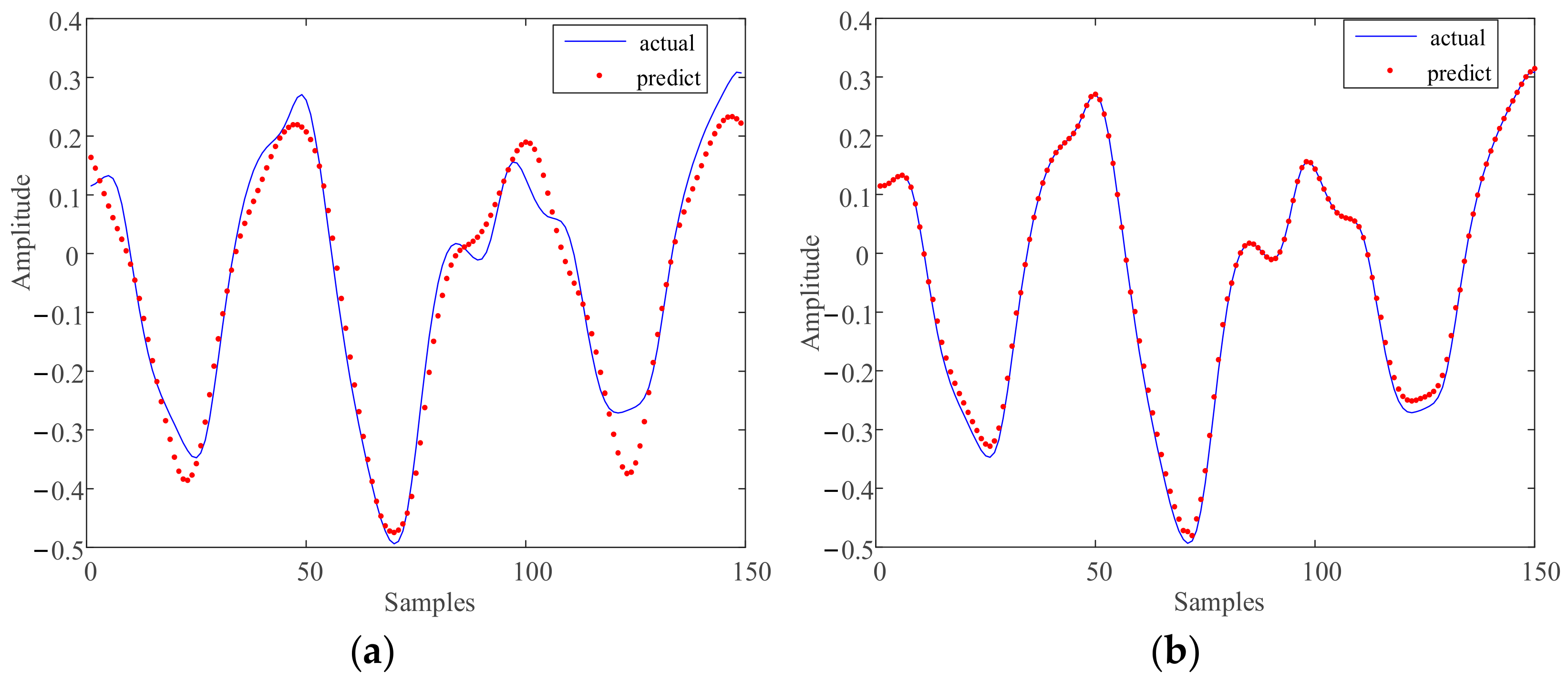
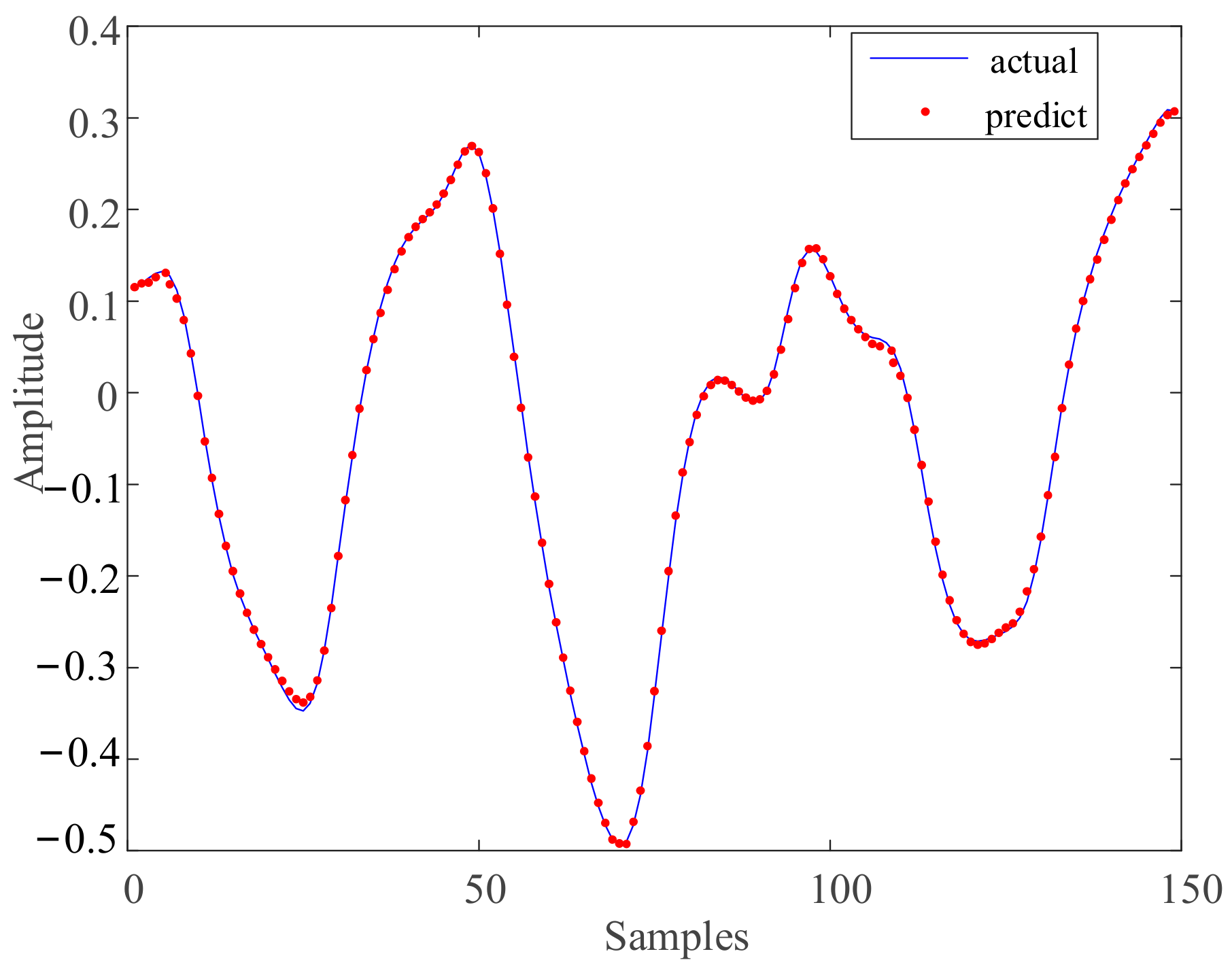
To verify the prediction performance of the proposed integration method, short-term predictions were made on chaotic time series data. During the experiment, the predicted data length was 150. The network parameters of the SVR method were set to ε = 0.01 and C = 20, and the Gaussian radial basis function was adopted. The parameters of the LSTM model were set as follows: the number of hidden layer units was 200, the maximum number of iterations was 100, the initial learning rate was 0.005, Adam was selected as the optimization function, and the weight coefficient of the fusion method was 0.5. The prediction results of the above two methods are shown in Figure 5, and Figure 6 shows the prediction result of the integration method.
The prediction effects of three prediction methods, including the LSTM prediction model, the SVR method, and the integration of LSTM and SVR, on the chaotic time series are compared in Figure 5 and Figure 6 and Table 1. Figure 5 shows that the prediction ability of the SVR model is higher than that of LSTM in the case of small samples; the RMSE of LSTM and SVR is 0.0419 and 0.0097, respectively, and R2 is 0.8905 and 0.9579, respectively. Figure 5 and Figure 6 show that the prediction effect of the integration of LSTM and SVR is better than both individually. It is known from Table 1 that the RMSE of the integration method drops to 0.0071, the MAPE reaches 1.54%, the SDAPE is 0.7141, the RWI is the closest to 1, and the corresponding R2 is also improved. In summary, the integration of LSTM and SVR is effective for small sample predictions.

4. Structural Damage Prediction of Engineering Vibration Signals

4.1. Structural Damage Trend Prediction Method

In this paper, the LSTM–SVR integrated model is used as a prediction model for structures. Since the instantaneous frequency can effectively reflect the changes in the health status of structures during their service life, the model is divided into three major parts in engineering vibration signal prediction: signal processing, data preprocessing, and LSTM–SVR network prediction. First, perform VMD and Hilbert transform on engineering data to obtain instantaneous frequency. Then, divide the obtained instantaneous frequency data into training sets and test sets and perform standardization processing. Finally, use the standardized data as input to the LSTM–SVR network model for data training and data prediction. Therefore, the method steps proposed in this article are as follows:
(1)
Select the acceleration vibration signal required for the experiment.
(2)
Use VMD to decompose the original signal.
(3)
Use Hilbert transform to obtain the instantaneous frequency of the decomposed component.
(4)
The instantaneous frequency of each component is analyzed to find out the high-order modal that characterizes the decrease in structural stiffness.
(5)
The feature frequencies are divided into training sets and test sets, which are standardized and used as input to LSTM–SVR. After learning the network model using the training sets, the test sets are used to predict structural health issues.
(6)
To illustrate the effectiveness of the LSTM–SVR prediction model in predicting structural health problems, it is compared with a single prediction method.
The prediction results of the chaotic time series data in the previous section show that the structural damage prediction of the integration of LSTM and SVR achieved excellent prediction results. To verify the effect of this method in actual vibration engineering data, actual engineering vibration data were used.

4.2. ASCE Structure Model

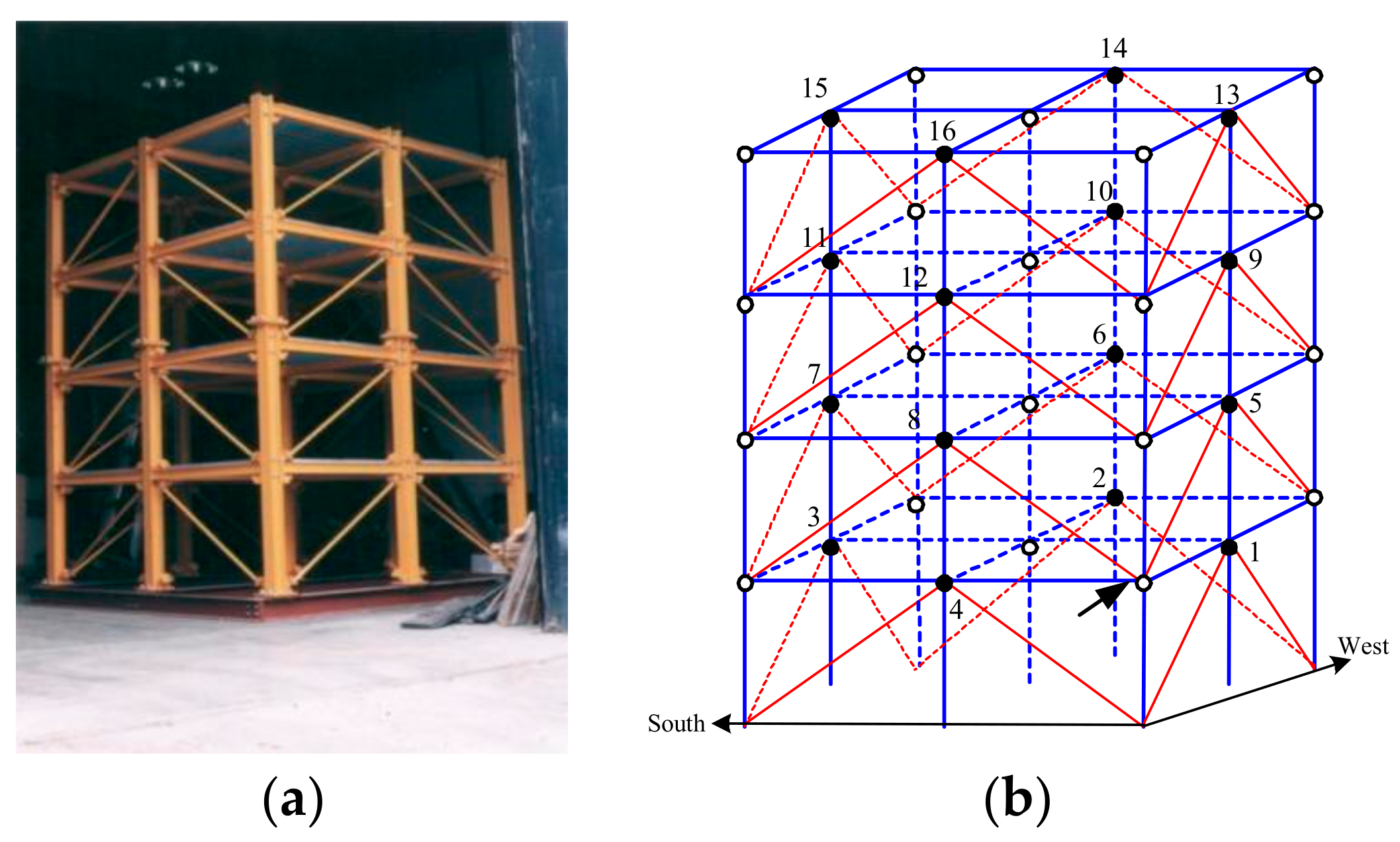
The method is used to analyze actual engineering vibration data to verify the effectiveness of this method. The shock data are taken from the series of experiments for the steel structure test model in the Earthquake Engineering Laboratory of the University of British Columbia (UBC) in 2002 [43]. The physical model is a four-story frame structure, each span is 1.25 m, the story height is 0.9 m, and the total height is 3.6 m as shown in Figure 7a. The diagonal supports are two parallel steel-threaded connections with a diameter of 12.7 mm. A 1000 kg concrete slab is placed on each span of the 1st to 3rd layers, and 750 kg concrete slabs are placed on each span of the four layers to make the mass distribution close to the actual engineering conditions. A total of 16 acceleration sensors are used to measure the vibration response signal of the structure, and the sampling frequency is 1000 Hz. Figure 7b shows the number and location of the measuring points. A 12-pound (5.44 kg) steel hammer is used to hit the structure, and the hit position is marked by an arrow in Figure 7b.

4.3. Prediction of Ill-Structured Problems under an External Incentive Environment

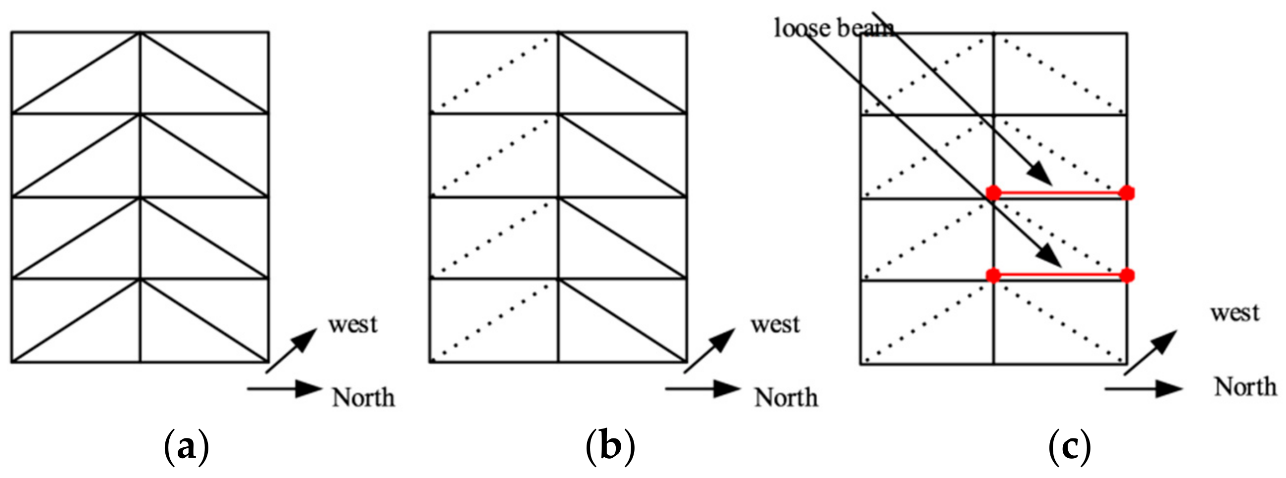
In order to verify the effectiveness of the proposed method in practical application, this method is used to analyze the actual engineering vibration data. The data used are Phase II IASC–ASCE, namely the second phase data of the vibration acceleration signal of the actual engineering of ASCE [44]. The actual engineering vibration data used in this section were generated with motor vibration excitation with a sampling frequency set at 200 Hz. The vibration signal collected with the acceleration sensor at the No. 6 detection point was selected as the research signal, and 3000 vibration data were used for analysis and research. Figure 8 shows the damage mode and the damage conditions. The conditions were selected as follows:
(a)
No damage;
(b)
All diagonal supports on the southeast side were removed (damage mode 1);
(c)
When all the diagonal supports of the structure were removed, the bolts at both ends of the beams on the first and second floors on the northeast side were loose (damage mode 2).
The collected acceleration vibration signals are shown in Figure 9. Hilbert–Huang transformation was performed on the acceleration signal, and then, the first component was taken for analysis. The transient frequency is shown in Figure 10.
As can be observed from Figure 10, under damage conditions, the instantaneous frequency shows a downward trend, and when there is no damage or the damage degree is slight, the overall fluctuation of the instantaneous frequency is relatively stable. As the damage degree deepens, the overall fluctuation amplitude also increases accordingly. The experimental results show that, when structural damage occurs, that is, when the structural stiffness decreases, the magnitude and amplitude of its instantaneous frequency will also change. It is further verified that instantaneous frequency can be used as a characteristic factor for structural ill-conditioned problems, and it also demonstrates the effectiveness of VMD combined with the Hilbert transform method.
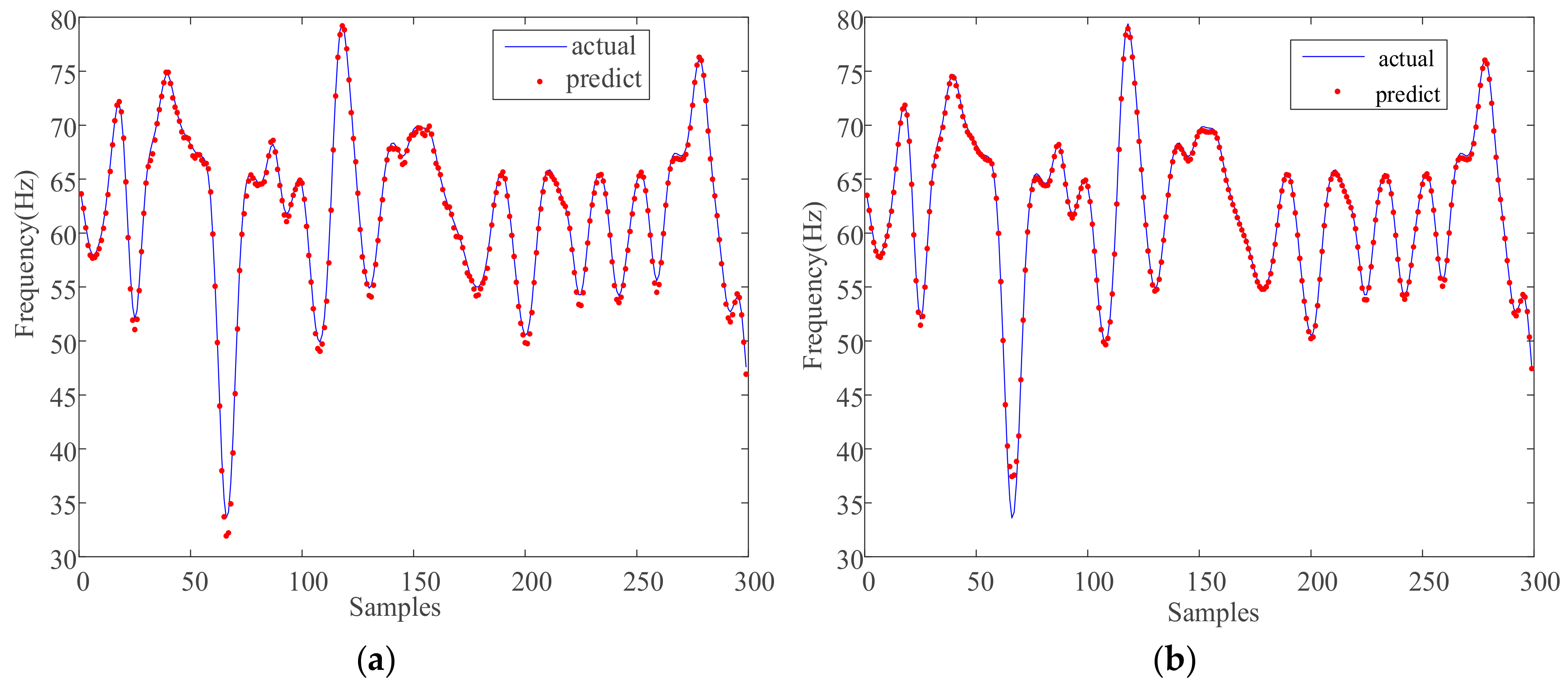
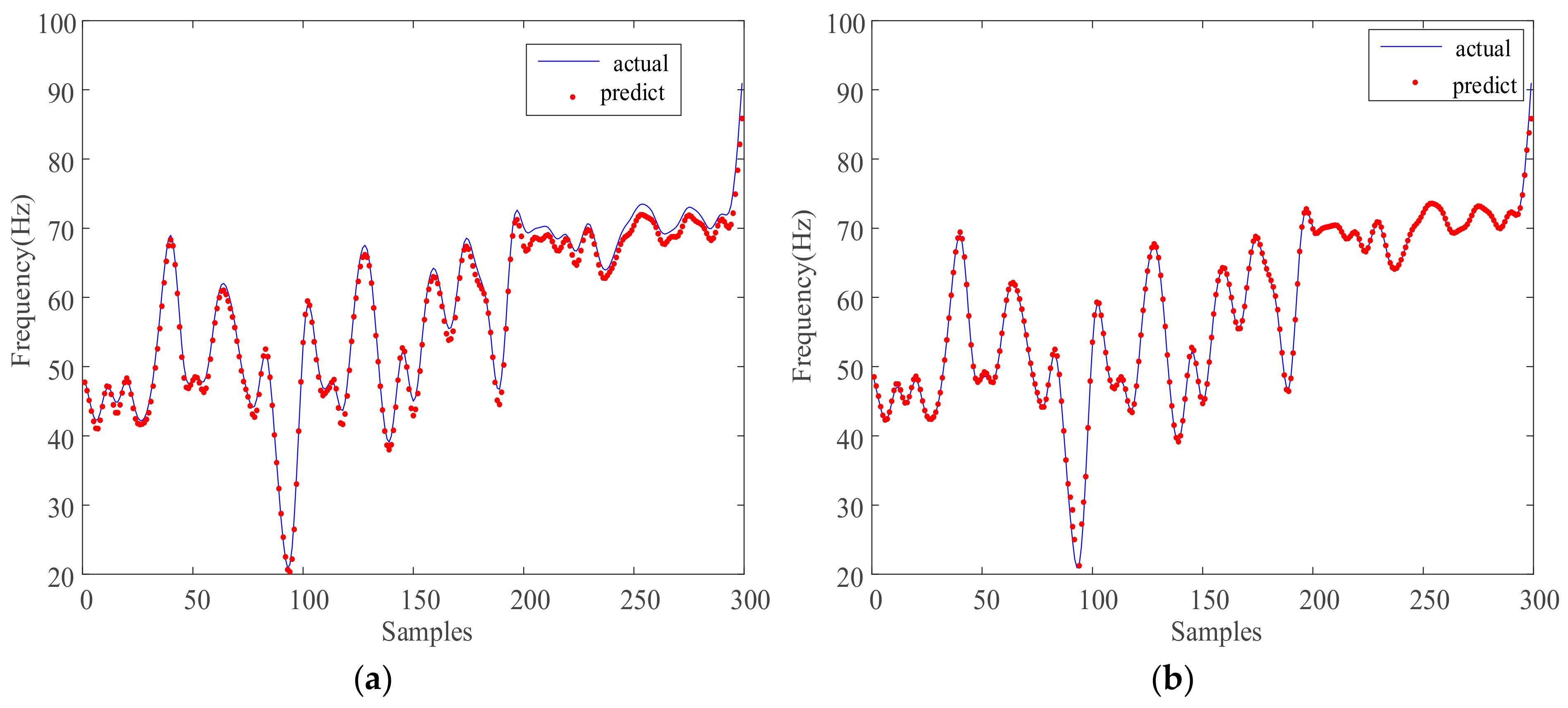
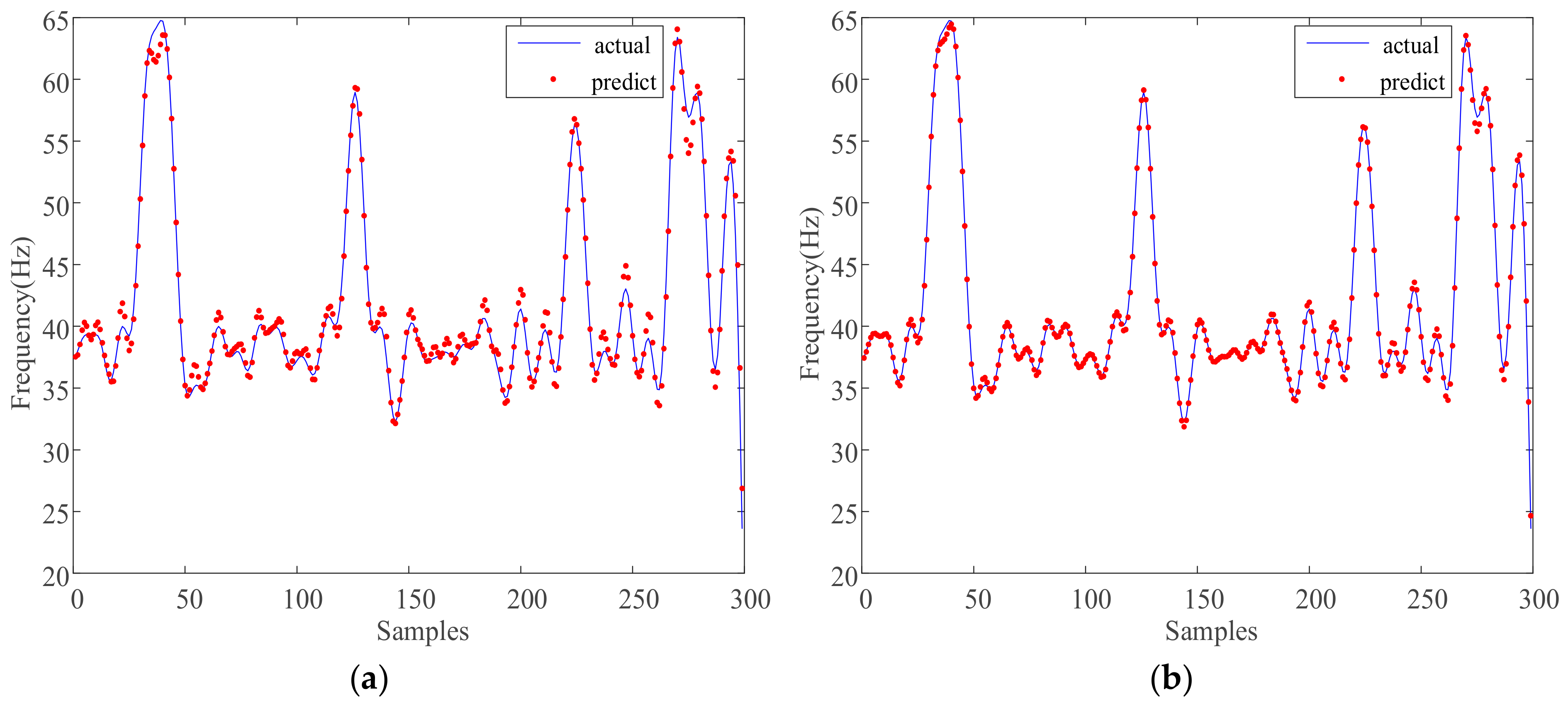
In the obtained transient frequency, 1000 data were taken for the fusion algorithm prediction. The first 700 were used as training data, and the last 300 were used as test data. The specific parameters of the fusion algorithm were set as follows: the weight coefficient w in the fusion method was 0.5, C and ε in the SVR method were 20 and 0.01, respectively, and the number of layered neurons in LSTM was 200 with 100 iterations. The predictions of the three working conditions are shown in Figure 11, Figure 12 and Figure 13. Herein, the solid line represents the actual value, and the dot represents the predicted value. In order to better verify the prediction effect, Table 2, Table 3 and Table 4 provide a comparison of performance evaluation with the LSTM algorithm.

4.4. Analysis of Prediction Results

As can be observed from Figure 11, Figure 12 and Figure 13, the model based on the integration of LSTM and SVR has high accuracy for data prediction under the three conditions. From Table 2, Table 3 and Table 4, it can be found that
(1)
The RMSE values of the single LSTM model in both the undamaged and two damaged states are 0.6549, 0.8156, and 0.8278, respectively, and based on the LSTM–SVR integration method, the RMSE values are 0.4740, 0.5346, and 0.4973, respectively. The integration method had a smaller prediction error for the engineering data, higher accuracy, and better prediction performance than the LSTM model.
(2)
The MAPE values of the single model under the three operating conditions are 0.59, 1.91, and 1.88. The MAPE values of the integrated method are 0.36, 0.25, 0.95. It indicated that the prediction error of the integrated method based on LSTM and SVR is smaller than that of the LSTM model.
(3)
The SDAPE values of the single model are 0.8635, 0.8321, and 0.8345, and those of the integrated method are 0.7641, 0.7452, and 0.7424. The SDAPE values of the three operating conditions under the integrated method are smaller than those of the LSTM model, which shows that the integrated method based on LSTM and SVR can improve the stability of prediction to a certain extent.
(4)
For the R2, the correlation between the actual prediction effect of the integrated algorithm and the actual value is also better, and the numerical value is closer to 1.
(5)
The RWI values of the three operating conditions under the integrated method are higher than those of the LSTM model, and the prediction accuracies of the integrated method have been improved 6.56%, 2.56%, and 3.7%, respectively.

5. Conclusions

This paper studied the prediction of structural damage trends based on the integration of the LSTM and SVR methods. The main conclusions were determined as follows:
(1)
VMD effectively avoids the modal aliasing phenomenon of EMD and can accurately extract the structural damage feature information.
(2)
According to numerous experiments, it is found that, when 0.5 was used as the weight coefficient, the R2 of the integration model reached the highest value of 0.9975, the prediction result of the integration method was closest to the actual value, and the prediction accuracy was the highest.
(3)
Through many experiments, in the integrated method validation experiment, the LSTM–SVR based integrated method has the highest prediction accuracy for smaller prediction samples compared to the other two single methods, and the coefficient of determination is 12% higher than the LSTM model.
(4)
In the prediction of actual engineering vibration data, among the RMSE, MAPE, SDAPE, R2, and RWI indicators, the integrated method has a smaller prediction error value for the engineering data, higher accuracy, more robustness, and better prediction performance compared to the LSTM network model, especially the average absolute percentage error. Compared to the LSTM model, the integrated method has improved the numerical value by an order of magnitude. It is of great significance to predict the damage trend of structures when there is less engineering vibration data in the future.
This finding is of great significance to the future prediction of structural damage trends when the amount of available engineering vibration data is low.

Funding

This research was funded by the Key Research and Development Program of Shaanxi Province grant number [2021GY-098].

Data Availability Statement

Some data and models generated during the study are available online at: http://cive.sea.wustl.edu/wusceel/ASCE.shm/experim_phase_2.htm (accessed on 6 June 2023).

Conflicts of Interest

The author declares no conflict of interest.

References

  1. Luo, Y.; Zhao, J. Research status and future prospects of space structure health monitoring. J. Build. Struct. 2022, 43, 16–28. [Google Scholar]
  2. Wang, H.; Guo, C.-L.; Wang, L. Structural health monitoring based on inner product matrix and deep learning. Eng. Mech. 2022, 39, 14–22, 75. [Google Scholar]
  3. Wang, J.; Zhang, X.; Chang, X.; Zhou, Z.; Wang, C.; Fu, Z.; Fu, B. Prediction model for blast-induced structural damage based on an optimized Bayes discriminant analysis model. Appl. Math. Model. 2022, 110, 338–366. [Google Scholar] [CrossRef]
  4. Mishra, M.; Lourenço, P.B.; Ramana, G.V. Structural health monitoring of civil engineering structures by using the internet of things: A review. J. Build. Eng. 2022, 48, 103954.1–103954.20. [Google Scholar] [CrossRef]
  5. Ganjdoust, F.; Kefal, A.; Tessler, A. A novel delamination damage detection strategy based on inverse finite element method for structural health monitoring of composite structures. Mech. Syst. Signal Process. 2023, 192, 110202.1–110202.34. [Google Scholar] [CrossRef]
  6. Vieira, M.; Henriques, E.; Snyder, B. Insights on the impact of structural health monitoring systems on the operation and maintenance of offshore wind support structures. Struct. Saf. 2022, 94, 102154.1–102154.14. [Google Scholar] [CrossRef]
  7. Pancholi, S.; Joshi, A.M. Improved Classification Scheme Using Fused Wavelet Packet Transform Based Features for Intelligent Myoelectric Prostheses. IEEE Trans. Ind. Electron. 2020, 67, 8517–8525. [Google Scholar] [CrossRef]
  8. Indhumathi, R.; Narmadha, T.V. Hybrid pixel based method for multimodal image fusion based on Integration of Pulse Coupled Neural Network (PCNN) and Genetic Algorithm (GA) using Empirical Mode Decomposition (EMD). Microprocess. Microsyst. 2022, 94, 104665.1–104665.10. [Google Scholar] [CrossRef]
  9. Dragomiretskiy, K.; Zosso, D. Variational mode decomposition. IEEE Trans. Signal Process. 2014, 62, 531–544. [Google Scholar] [CrossRef]
  10. Wu, J. Short-Term Power Load Forecasting Based on VMD and Improved Extreme Learning Machine; Xi’an University of Technology: Xi’an, China, 2019. [Google Scholar]
  11. Zhang, Y.G.; Zhao, Y.; Gao, S. A novel hybrid model for wind speed prediction based on VMD and neural network considering atmospheric uncertainties. IEEE Access 2019, 7, 60322–60332. [Google Scholar] [CrossRef]
  12. Zhang, W.; Yang, Q.; Kumar, M.; Mao, Y. Application of Improved Least Squares Support Vector Machine in the Forecast of Daily Water Consumption. Wirel. Pers. Commun. 2018, 102, 3589–3602. [Google Scholar] [CrossRef]
  13. Zhuo, Y.; Han, Z.; Duan, J.; Jin, H.; Fu, H. Estimation of vibration stability in milling of thin-walled parts using operational modal analysis. Int. J. Adv. Manuf. Technol 2021, 115, 1259–1275. [Google Scholar] [CrossRef]
  14. Shahvaroughi Farahani, M.; Razavi Hajiagha, S.H. Forecasting stock price using integrated artificial neural network and metaheuristic algorithms compared to time series models. Soft Comput. 2021, 25, 8483–8513. [Google Scholar] [CrossRef]
  15. Wang, Y.; Zhu, Z.; Sha, A.; Hao, W. Low cycle fatigue life prediction of titanium alloy using genetic algorithm-optimized BP artificial neural network. Int. J. Fatigue 2023, 172, 107609.1–107609.11. [Google Scholar] [CrossRef]
  16. Wang, L.; Wang, Y.-L.; An, Z.-Y. Echo state networks with improved particles warm Optimization algorithm for electricity demand foecasting. Comput. Eng. Sci. 2022, 44, 1457–1466. [Google Scholar]
  17. Bahareh, A.; Salim, L. Hybrid deep learning and GARCH-family models for forecasting volatility of cryptocurrencies. Mach. Learn. Appl. 2023, 12, 100465. [Google Scholar]
  18. Xiao, C.; Chen, N.; Hu, C.; Wang, K.; Gong, J.; Chen, Z. Short and mid-term sea surface temperature prediction using time-series satellite data and LSTM-Ada Boost combination approach. Remote Sens. Environ. 2019, 233, 111358. [Google Scholar] [CrossRef]
  19. Luo, H.; Huang, M.; Zhou, Z. A dual-tree complex wavelet enhanced convolutional LSTM neural network for structural health monitoring of automotive suspension. Measurement 2019, 137, 14–27. [Google Scholar] [CrossRef]
  20. He, M.; Zhou, Y.; Li, Y.; Wu, G.; Tang, G. Long short-term memory network with multi-resolution singular value decomposition for prediction of bearing performance degradation. Measurement 2020, 156, 107582. [Google Scholar] [CrossRef]
  21. Li, P.; Zhang, Z.; Xiong, Q.; Ding, B.; Hou, J.; Luo, D.; Rong, Y.; Li, S. State-of-health estimation and remaining useful life prediction for the lithium-ion battery based on a variant long short term memory neural network. J. Power Sources 2020, 459, 228069. [Google Scholar] [CrossRef]
  22. Liu, Y.; Wang, K.; Li, L. Prediction of watershed pollutant flux based on LSTM neural network. J. Hydroelectr. Eng. 2020, 10, 72–81. [Google Scholar]
  23. Zhao, J.; Bai, G.; Li, Y. Short-term wind power prediction based on CNN-LSTM. Autom. Instrum. 2020, 41, 37–41. [Google Scholar]
  24. Yang, Y.; Wang, B.; Liu, Y.; Xi, J. Temperature prediction based on space-time optimization LSTM deep learning network. J. Xuzhou Inst. Technol. 2020, 35, 44–49. [Google Scholar]
  25. Fang, W.; Zhuo, W.; Song, Y.; Yan, J.; Zhou, T.; Qin, J. ∆free-LSTM: An error distribution free deep learning for short-term traffic flow forecasting. Neurocomputing 2023, 526, 180–190. [Google Scholar] [CrossRef]
  26. Lyu, G.; Zhang, H.; Miao, Q. Parallel State Fusion LSTM-based Early-cycle Stage Lithium-ion Battery RUL Prediction Under Lebesgue Sampling Framework. Reliab. Eng. Syst. Saf. 2023, 236, 109315. [Google Scholar] [CrossRef]
  27. Li, Q.; Guan, X.; Liu, J. A CNN-LSTM framework for flight delay prediction. Expert Syst. Appl. 2023, 227, 120287. [Google Scholar] [CrossRef]
  28. Liu, W.; Pan, J.; Ren, Y.; Wu, Z.; Wang, J. Coupling prediction model for long-term displacements of arch dams based on long short-term memory network. Struct. Control Health Monit. 2020, 27, 2548. [Google Scholar] [CrossRef]
  29. Luo, H.; Huang, M.; Zhou, Z. Integration of Multi-Gaussian fitting and LSTM neural networks for health monitoring of an automotive suspension component. J. Sound Vib. 2018, 428, 87–103. [Google Scholar] [CrossRef]
  30. Li, K.; Zhang, Z.; Guo, H.; Li, W.; Yan, Y. Prediction method of pipe joint opening-closing deformation of immersed tunnel based on singular spectrum analysis and SSA-SVR. Appl. Ocean. Res. 2023, 135, 103526. [Google Scholar] [CrossRef]
  31. Yu, D.; Liu, M. Non-invasive Load Decomposition of Substation Based on Deep Convolutional Neural Network and Support Vector Machine. Electr. Power Sci. Eng. 2020, 36, 24–30. [Google Scholar]
  32. Li, J.; Zhu, D.; Li, C. Comparative analysis of BPNN, SVR, LSTM, Random Forest, and LSTM-SVR for conditional simulation of non-Gaussian measured fluctuating wind pressures. Mech. Syst. Signal Process. 2022, 178, 109285. [Google Scholar] [CrossRef]
  33. Pan, Y.; Jin, X.; Li, Y.; Chen, D.; Zhou, J. A Study on the Prediction of Book Borrowing Based on ARIMA-SVR Model. Procedia Comput. Sci. 2021, 188, 93–102. [Google Scholar] [CrossRef]
  34. Luo, J.; Gong, Y. Air pollutant prediction based on ARIMA-WOA-LSTM model. Atmos. Pollut. Res. 2023, 14, 101761. [Google Scholar] [CrossRef]
  35. Jitendra, K.; Rimsha, G. Long Short Term Memory Recurrent Neural Network (LSTM-RNN) Based Workload Forecasting Model For Cloud Datacenters. Procedia Comput. Sci. 2018, 125, 676–682. [Google Scholar]
  36. Ding, S.; Xu, Y.; Sun, T.; Yu, J.; Wang, L.; Zhu, R. Roadside Unit Visibility Prediction Method Based on SVR. Eng. Lett. 2023, 31, 419–434. [Google Scholar]
  37. Zhang, X.; Ruan, J.; Rong, Q. Multiregion Indirect Resistivity Detection Method for Oil-impregnated Paper in Power Transformer Based on SVR. High Volt. Eng. 2021, 47, 1020–1027. [Google Scholar]
  38. Liu, H. Stock Index Futures Price Forecasting Scheme Based on LSTM-SVR Hybrid Model; Shanghai Normal University: Shanghai, China, 2020. [Google Scholar]
  39. Liu, Y.; Tian, T.; Wang, C. Trend prediction of structural health status based on EWT and FESN. Chin. J. Appl. Mech. 2019, 36, 645–651. [Google Scholar]
  40. Yang, Y.; Xu, L.; Han, H.; Ren, Z.; Wu, K.; Liu, F. Soft measurement and prediction of refrigerant leakage based on SVR-LSTM. Int. J. Refrig. 2023, in press. [Google Scholar] [CrossRef]
  41. Ye, Y.; Wang, L.; Wang, Y.; Qin, L. An EMD-LSTM-SVR model for the short-term roll and sway predictions of semi-submersible. Ocean. Eng. 2022, 256, 111460. [Google Scholar] [CrossRef]
  42. Raja, M.N.A.; Shukla, S.K. Predicting the settlement of geosynthetic-reinforced soil foundations using evolutionary artificial intelligence technique. Geotext. Geomembr. 2021, 49, 1280–1293. [Google Scholar] [CrossRef]
  43. Available online: http://cive.seas.wustl.edu/wusceel/ASCE.shm/experim_phase_2.htm (accessed on 1 August 2006).
  44. Ching, J.; Beck, J.L. Bayesian Analysis of the Phase II IASC-ASCE Structural Health Monitoring Experimental Benchmark Data. J. Eng. Mech. 2004, 130, 1233–1244. [Google Scholar] [CrossRef]
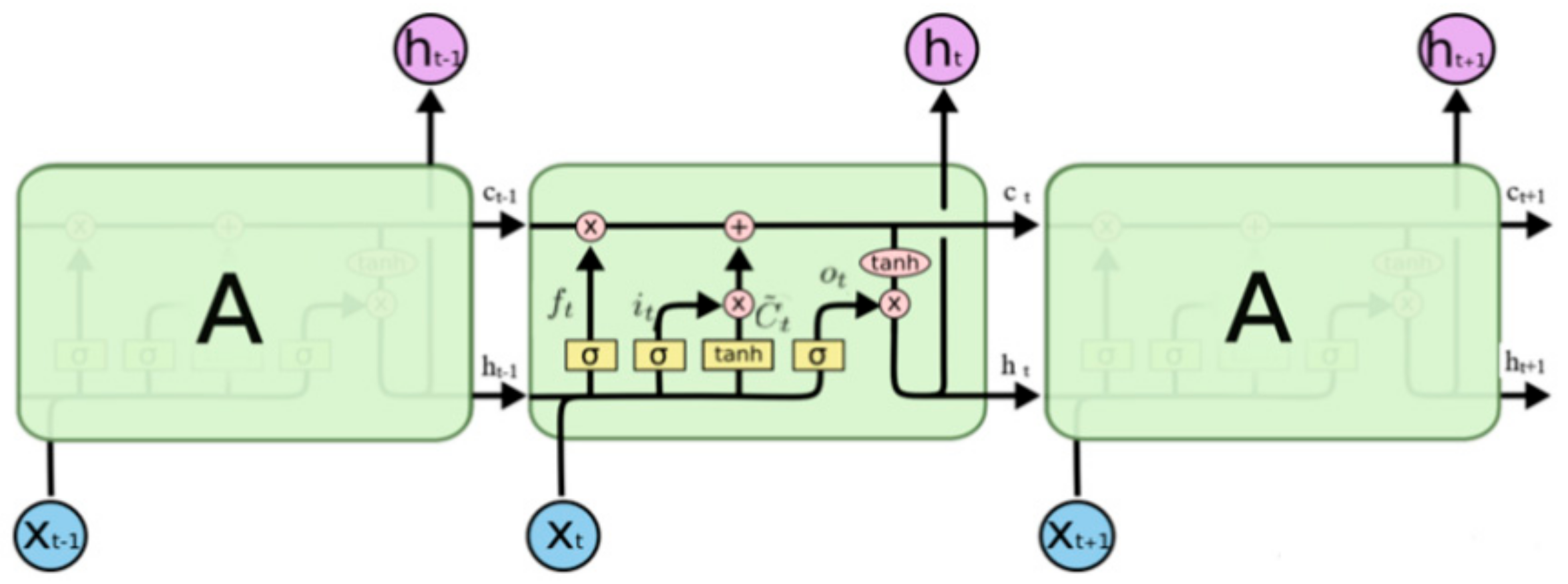
Figure 1. Schematic diagram of LSTM.
Applsci 13 07135 g001
Figure 2. Integrated prediction box of the LSTM and SVR models.
Applsci 13 07135 g002
Figure 3. Flow of the LSTM model and SVR fusion algorithm.
Applsci 13 07135 g003
Figure 4. R2 corresponding to weight coefficient.
Applsci 13 07135 g004
Figure 5. Comparison of short-term prediction effects of a chaotic time series. (a) LSTM prediction. (b) SVR prediction.
Applsci 13 07135 g005
Figure 6. Prediction effects of a chaotic time series of the integration method.
Applsci 13 07135 g006
Figure 7. Experimental model, node number, and hit position. (a) Steel-frame quarter-scale model structure. (b) Diagram of the analytical model.
Applsci 13 07135 g007
Figure 8. Three working modes. (a) No damage condition. (b) Damage mode 1. (c) Damage mode 2.
Applsci 13 07135 g008
Figure 9. Acceleration vibration signals under three working conditions.
Applsci 13 07135 g009
Figure 10. The transient frequency corresponding to acceleration under three working conditions.
Applsci 13 07135 g010
Figure 11. Short-term prediction results of non-destructive conditions. (a) LSTM model. (b) Integration method.
Applsci 13 07135 g011
Figure 12. Short-term prediction results after removing all the diagonal supports on the southeast side. (a) LSTM model. (b) Integration method.
Applsci 13 07135 g012
Figure 13. Short-term prediction results of bolts loosening at both ends of the first and second floor beams on the northeast side without any diagonal support. (a) Prediction results of LSTM. (b) Integration method.
Applsci 13 07135 g013
Table 1. Comparison of prediction effects of the integration method.
RMSEMAPE(%)SDAPER2RWIOperation Time/s
LSTM0.04191.530.85210.89050.846581.134
SVR0.00971.950.80110.95790.86370.385
Integration method0.00711.540.71410.98890.9021108.213
Table 2. Evaluation of prediction performance under non-destructive conditions.
RMSEMAPE(%)SDAPER2RWIOperation Time/s
LSTM0.65490.590.86350.98210.896592.533
Integration method0.47400.360.76410.99590.962194.879
Table 3. Evaluation of the damage prediction performance after removing all the diagonal supports on the southeast side.
RMSEMAPE(%)SDAPER2RWIOperation Time/s
LSTM0.81561.910.83210.98340.946594.595
Integration method0.53460.250.74520.99590.972197.840
Table 4. Prediction performance evaluation of bolts loosening at both ends of the first and second floor beams on the northeast side without any diagonal support.
RMSEMAPE(%)SDAPER2RWIOperation Time/s
LSTM0.82781.880.83450.98500.9431103.198
Integration method0.49730.950.74240.99600.980197.302
Disclaimer/Publisher’s Note: The statements, opinions and data contained in all publications are solely those of the individual author(s) and contributor(s) and not of MDPI and/or the editor(s). MDPI and/or the editor(s) disclaim responsibility for any injury to people or property resulting from any ideas, methods, instructions or products referred to in the content.