Abstract
Data-driven models have been successfully applied to flood prediction. However, the nonlinearity and uncertainty of the prediction process and the possible noise or outliers in the data set will lead to incorrect results. In addition, data-driven models are only trained from available datasets and do not involve scientific principles or laws during the model training process, which may lead to predictions that do not conform to physical laws. To this end, we propose a flood prediction method based on data-driven and knowledge-guided heterogeneous graphs and temporal convolutional networks (DK-HTAN). In the data preprocessing stage, a low-rank approximate decomposition algorithm based on a time tensor was designed to interpolate the input data. Adding an attention mechanism to the heterogeneous graph module is beneficial for introducing prior knowledge. A self-attention mechanism with temporal convolutional network was introduced to dynamically calculate spatiotemporal correlation characteristics of flood data. Finally, we propose physical mechanism constraints for flood processes, adjusted and optimized data-driven models, corrected predictions that did not conform to physical mechanisms, and quantified the uncertainty of predictions. The experimental results on the Qijiang River Basin dataset show that the model has good predictive performance in terms of interval prediction index (PI), RMSE, and MAPE.
1. Introduction
Effective flood forecasting methods contribute to flood control and disaster emergency management [1]. From the perspective of data analysis, flood forecasting based on data-driven models is essentially time-series data prediction [2]. At present, flood time-series data prediction research based on the data driven model mainly faces the following challenges [3]. The inherent nonlinearity of the flood process and the uncertainty of the predicted results bring risks to flood control decision-making. The DL model is only trained from available datasets and cannot reasonably utilize scientific principles or laws during the model training process, which may lead to unreasonable predictions. In the actual measurement, the quality of the collected data cannot be guaranteed, and the data may have noise or outliers. Due to the data-driven nature of the learning process, the robustness and versatility of the learning results are poor, resulting in completely incorrect results [4]. Therefore, many researchers have proposed using data-driven and knowledge-guided models to address the aforementioned challenges [5].
The effective implementation of the above data-driven and knowledge-guided prediction theory relies on machine learning prediction models. Among these, depth neural networks are one of the most representative machine learning methods. Flood prediction methods of deep neural networks mainly include RNN-based prediction methods [6], LSTM-based prediction methods [7], and GRU-based prediction methods [8]. The above intelligent methods mainly start from the perspective of Euclidean data regression, ignoring the important physical structure of the basin itself and the spatiotemporal characteristics of data features. Accurate flood prediction needs to be based on the physical structure of the watershed itself and the spatiotemporal characteristics of the data [9]. The prediction method based on the graph neural network model [10] extends the deep learning model to non-Euclidean space, and can extract the spatiotemporal characteristics of the flood physical field in parallel. It fully considers the physical structure within the watershed, namely, various spatial topological connections. At present, research on flood forecasting methods based on graph neural networks mainly focuses on isomorphic and heterogeneous graphs [11]. Among these, isomorphic graphs only have one type of node and edge, which corresponds to the field of flood prediction, that is, only one type of station and its runoff direction relationship are predicted, which clearly does not comply with the physical mechanism of flood basins. Considering the spatiotemporal complexity of flood processes, modeling them as heterogeneous maps containing multiple types of nodes and edges can achieve more detailed and comprehensive flood processes. By combining the different attribute features of different hydrological stations to extract a wide range of spatiotemporal features, more accurate flood spatiotemporal prediction can be achieved [12].
Recurrent neural networks are used to solve the problem of training sample inputs as continuous sequences with different sequence lengths. However, it has short-term memory problems, cannot handle long input sequences, and is prone to gradient explosion or gradient disappearance [13]. The gradient problem of Recurrent Neural Network (RNN) has been solved for a certain gradient problem in Long Short-Term Memory (LSTM), but the requirements for data must be time-dependent. In addition, LSTM is unable to perform parallel operations and has very high hardware requirements during the training process. Temporal Convolutional Network (TCN) can run in parallel. Their flexible receptive field and stable gradient are more suitable for capturing the characteristics of long time-series data [14]. In addition, the convolutional core of the TCN network is shared in one layer and the memory usage during training is low [15].
Currently, research on data-driven and knowledge-guided floods mostly relies on deterministic point prediction to output prediction results. This method may not eliminate absolute prediction errors and lacks effective evaluation methods [16]. Interval prediction can effectively quantify the uncertainty of flood forecasting, thereby more reasonably estimating potential uncertainties and risks. At present, the representative interval prediction method is upper- and lower-bound estimation (LUBE) [17]. Research on this mainly focuses on the construction of interval prediction functions and the optimization of the training process. However, the above methods may still require multiple iterations to use the PI evaluation index as the objective function, resulting in high computational resource consumption. In addition, the above method performs interval prediction without losing the original input data. When the input data are partially missing, the output accuracy of the above model may be affected to a certain extent. The phenomenon of missing original input data is common in the field of flood forecasting [18].
With the lack of input data in flood forecasting, the current solutions mainly include two types. One method is to directly delete the missing data in the entire section [19]. Another method is to use algorithms to convert incomplete data into complete data, which is the data interpolation method [20]. At present, the more popular technology in the field of flood time-series data preprocessing is tensor-based decomposition and interpolation technology [21]. Chen et al. [22] completed data interpolation work based on the Tucker decomposition three-process framework by discovering spatiotemporal patterns and underlying structures from incomplete data. Zhou et al. [23] proposed a new incremental algorithm, while Che et al. [24] introduced the idea of adaptive randomization to handle it. Yuan et al. [25] completed tensor processing using the low-rank structure of the TR potential space, which is robust to model selection. In addition, we note that in the face of time-varying massive hydrological heterogeneous and complex data, the above incremental methods do not deeply consider the sparsity of data decomposition. This will affect the accuracy of model predictions and the overall computational resource consumption of the prediction model.
The main limitations of flood time-series prediction based on data-driven models are as follows. Intelligent data-driven flood prediction models are easily affected by data noise in practical engineering. Then, the presence of missing data makes the model prone to unreasonable or unrealistic predictions, and existing tensor preprocessing methods cannot effectively solve the sparsity problem of flood data. In addition, data-driven models only consider flood prediction from the perspective of data, lacking consideration and research on the spatiotemporal characteristics of the flood process itself, and cannot avoid prediction errors caused by a lack of physical knowledge. For this reason, we propose data-driven and knowledge-guided heterogeneous graphs and temporal convolution networks for flood forecasting. The main contributions of this article are summarized as follows.
- (1)
- This article proposes a data-driven and knowledge-based dual-drive flood prediction model, which optimizes the initial conditions of the model through heterogeneous graph modules and introduces prior knowledge of the watershed. TCN with integrated attention is used to fit the model, significantly reducing data noise and enhancing the robustness of the model.
- (2)
- The proposed model effectively integrates the guiding framework technology of flood physics theory into data-driven models, and introduces physical constraints that comply with the physical laws of flood flow prediction principles, solving the problem of errors in common data-driven model predictions that do not conform to physical knowledge.
- (3)
- This article first discusses the combination of tensor low-rank approximation data preprocessing methods and flood prediction mechanisms to effectively compensate for tensor sparsity.
- (4)
- It is recommended to use interval prediction output architecture to quantify the output error of the model, in order to improve the accuracy of flood time-series data prediction. The experimental results show that compared to the baseline, the proposed model improves the index of PI coverage probability (PICP) by 11.4%.
The rest of this article is organized as follows. Section 2.1 presents preliminaries for the proposed model, Section 2.2 introduces the proposed DK-HTAN model, and Section 3 describes the performance evaluation and results. Section 4 discusses the model results, and Section 5 provides summary opinions and future work.
2. Materials and Methods
2.1. Preliminaries
2.1.1. Tensor Decomposition
Tensor can be said to be a higher-order extension of matrix. In this paper, we use is the tensor, where d is the order. We use to represent the component of the third-order tensor Y, where , and m is called the module of tensor . The more commonly used tensor decomposition method is CPD, where the tensor Y can be further expressed as the sum of r ranks, for example, . Each component can be expressed as , where . For non-convex problems in tensor processing [26], we mainly solve them by regularization method.
where is the estimated value of tensor component represents Frobenius parameterization. In our research, tensor decomposition technology is mainly used to analyse the internal relationship of hydrological longitudinal data.
2.1.2. Graph Convolution
A graph convolution network [27] is the application of a convolution operation on graph neural network. The core information propagation formula of its network is as follows:
where is the first-level input, is the L-level feature in GCN, and is the L-level parameter in GCN. Through continuous training, it is determined that not only can the characteristics of a node be given weight but also the nodes and their neighbors can be given weight during information transmission. σ Is a nonlinear activation function, and the adjacency matrix is calculated as follows: , where D is and the degree matrix of can be calculated by the formula:
For a characteristic of a node in the graph at a certain time, and adjacency matrix , we can obtain the Laplace matrix . In order to further standardize the calculation, we can use the normalized Laplace matrix .
2.1.3. Temporal Convolution
The convolution neural network is the foundation of TCN [28]. TCN, in contrast to the general convolutional neural network (CNN), uses the structure of dilated causal convolution and residual block, allowing it to extract features from large-sample time series and realize prediction. It also successfully addresses the issue of a deep network’s performance degrading during the network training process.
Assume the given input sequence is . Expected predicted output is . The relationship between predicted output and input sequence is:
where is only related to the input sequence x at time t and before time t related to . Any future input is irrelevant. TCN modelling is to establish the mapping relationship f between the input and output sequence. Its objective function is to minimize the actual output and predicted value . The network will increasingly compress all information over time because the hidden layer state is often represented by a particular dimension of a tensor. However, this nondifferential compression will somewhat diminish the time difference between input features and might not draw attention to crucial details in rainfall history data. Therefore, the capacity to distinguish TCN needs to be improved with the relevant changes.
2.2. Methods
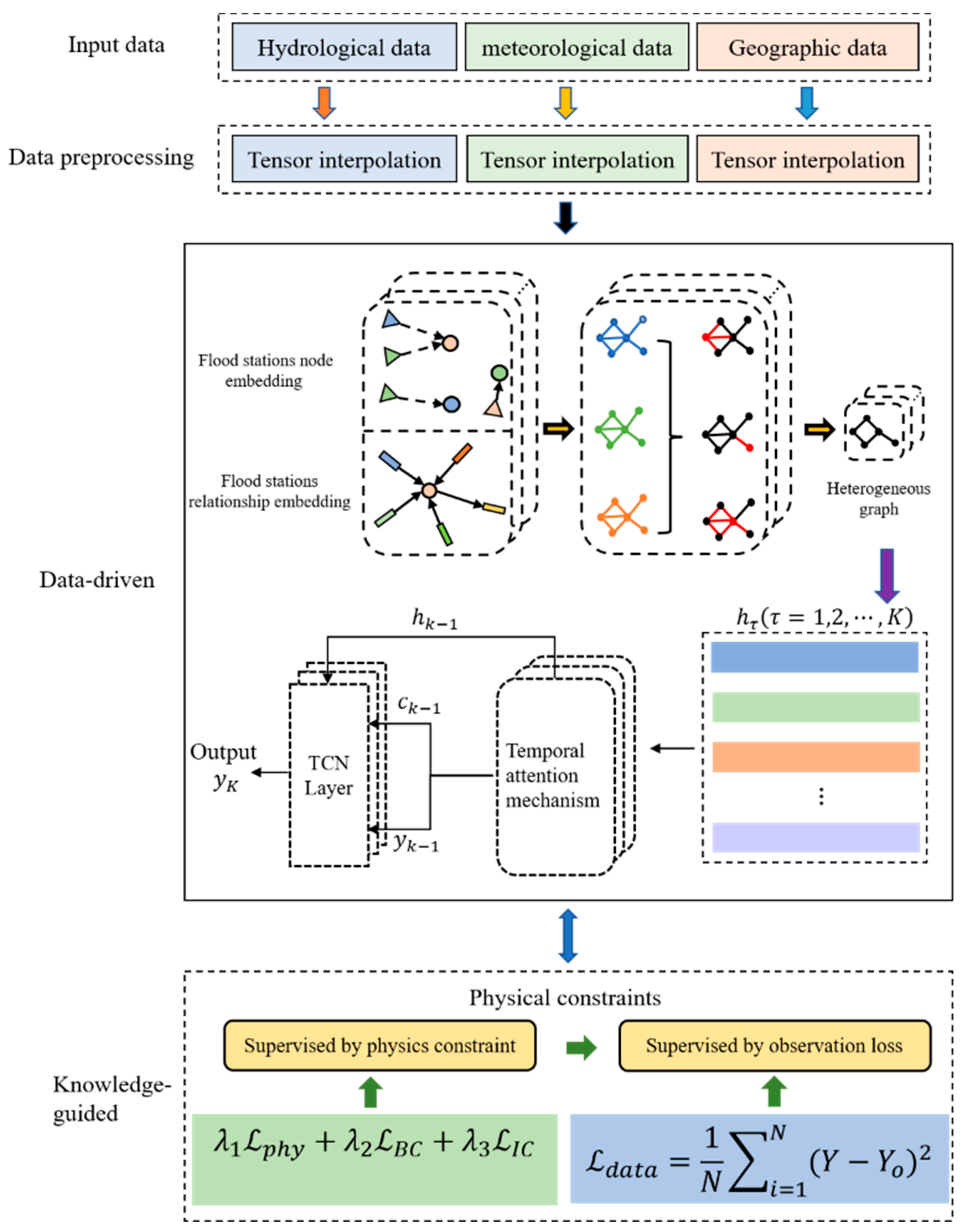
Generally speaking, flood data have rich temporal and spatial characteristics. Based on this, we propose data-driven and knowledge-guided based heterogeneous graphs and temporal convolution networks (DK-HTAN). The specific structure is shown in Figure 1 below. Firstly, in the data preprocessing stage, we studied data with sparsity from the perspective of tensor low-rank approximation to construct normal interpolation. Secondly, in order to better introduce prior features of hydrological spatiotemporal data, an attention mechanism was introduced in the heterogeneous graph module to learn spatial feature representation, capturing hidden spatial relationships in flood data of each hydrological station. Then, an improved self-attention mechanism was added to TCN, calculating the impact factors of individual features, generating dynamic spatiotemporal correlation weight tensors, and capturing the temporal characteristics of flood data of hydrological stations. Finally, we introduced the physical constraints of watershed floods to regulate and optimize the model. We will provide a detailed introduction to the functions of each module.

Figure 1.
Model diagram of data-driven and knowledge-guided based heterogeneous graphs and temporal convolution networks (DK-HTAN).
2.2.1. Knowledge-Guided Framework Based on Physical Constraints
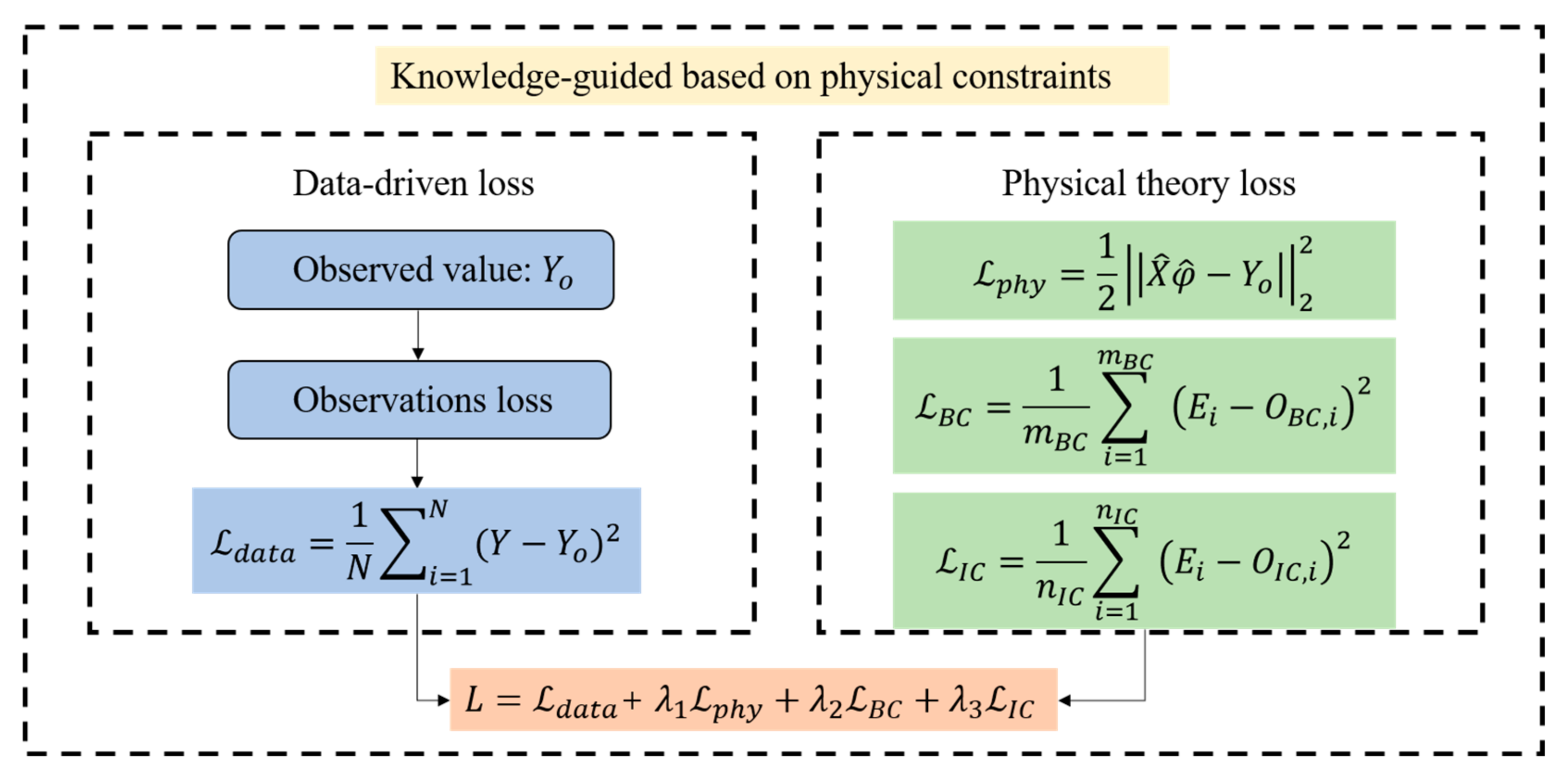
When data-driven models are used for flood prediction, only from a data perspective, the known physical constraints between observed and unobserved processes cannot be utilized, and they lack discrimination against some common-sense errors. The added physical constraint complies with the physical laws of the corresponding watershed derived from the observation data. A penalty term in the neural network loss function can be used to describe the degree of deviation between the neural network prediction and the constraint when this physical constraint is introduced into the model, particularly when the physical mechanism has been simplified into straightforward control equations. In this study, the theoretical guidance framework was better demonstrated by taking the flood discharge problem in small and medium-sized watershed areas as an example. In sections with tributaries, if the inflow of tributaries is large, the interference between the floods of the main and tributaries cannot be ignored. Therefore, this article adds the physical equation of the synthetic flow method for flood forecasting in river sections as a constraint mechanism. The specific structure is shown in Figure 2. River section flood forecasting is based on the operation and deformation laws of flood waves in the river section, using the measured flow of the upper section of the river section to predict the future flow of the lower section of the river section. This article mainly uses the synthetic flow method for river section floods. The specific formula is shown in Equation (5) below.
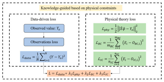
Figure 2.
Loss framework guided by physical constraints of knowledge-guided module.
Qt represents the flow of downstream stations at time t; represents the time when the flood from each i-th upstream station reaches the downstream station; n represents the number of upstream main and tributary stations; and Qi represents the flow of the i-th upstream station at time t.
Under different water conditions, the time for flow propagation from upstream stations to downstream stations may vary, but the difference is within a certain time range, and the span of that time range is limited. Therefore, this article estimates the as the center, expand a time range forward to form a time window, and synthesize the linear combination of flow rates of all upstream stations within the time window as a prediction of flow rates of downstream stations. The specific relationship formula is:
M represents the time span of opening the window forward, and the size of the time window can be expressed as L = 2m + 1; φ is the weight coefficient of traffic at each time within the window. Record the number of stations on the upstream main and tributaries as n, and L is the time span for window opening. There are already N corresponding flow data for upstream and downstream stations in the historical data; is the matrix formed by the flow data of the i-th upstream station within N time windows.
represents the linear combination coefficient of flow data within the time window of the i-th upstream station; represents N flow data of downstream stations. The matrix expression can be expressed as:
Set , then the matrix representation can be expressed as , where and is a coefficient to be determined. The objective function of the control equation can be determined as:
According to the Frobenius norm’s partial derivative rule, for the objective function , the gradient of parameter is:
In addition, the penalty terms for the boundary condition and initial condition are defined as:
mBC and nIC represent the number of boundary point and initial points, respectively; OBC and OIC are the observation value of boundary conditions and initial conditions, respectively; and represents the i-th prediction of the neural network.
The objective function of the control equation is introduced into the loss function of the network to avoid the violation of physical mechanics by the final prediction. By using the equation, the model loss can be obtained as follows:
Among , , is a penalty parameter, which controls the weight of each item in the loss function to the hyperparameter.
We suggest the discretization of equations, which is comparable to the finite element analysis in computational fluid dynamics and can change the control equations into more easily handled discrete forms, in order to better incorporate the physical constraints into the neural network. The partial differential equation is changed into a differential structure during the discretization process, which is based on the concept of finite difference. The flood control equation (Equation (12)) is discretized based on the second-order central difference scheme along the X and Y dimensions and the first-order backward Euler scheme along the t dimension. Finally, the discrete equation of flood was obtained, as shown in Equation (13):
Xi, Yo and T represent the coordinates of the constraint’s configuration points in space and time; Δx, Δy, and ΔT represent the difference interval in the Xi, Yo and T direction; FP represents the coordinates of the constraint patches around the configuration points Xi, Yo and T; and represents the velocity of waves and currents. In Equation (8), the configuration points are represented in bold.
The physical mechanism that the model should adhere to is described by the discretization Equation (13) in detail. When the predictions of each point in the constrained fulfil the relationship described in Equation (13), the constrained satisfies the limitations of control Equation (12). It should be noted that the discretization equation might not be satisfied by the direct prediction of the neural network in the constraints in Equation (13) are essentially soft constraints because the theoretical guidance framework. We modify the predictions in the constraints so that the results are consistent with the constraints related to the control equation, and also most similar to the original predictions in Equation (12).
2.2.2. Pretreatment of Data Tensioning
Research has shown that algorithms based on tensor decomposition interpolation can extract effective information from multiple dimensions of input hydrological, meteorological, and geographic information data, fully considering the correlation and complementarity between different dimensions, and effectively improving the accuracy of model predictions [29]. Due to the sparsity of data, the tensor decomposition interpolation algorithm proposed in this paper mainly studies tensor rank. Usually, tensor column rank (TT rank) is used to recover low-rank components. To make TT rank more effective, we use TT factorization and parallel matrix factorization techniques to assign different importance to different elements of the tensor. Specifically, based on tensor column decomposition and matrix decomposition, the optimization objectives for tensor complete problems are as follows:
Here, the pattern matrix is obtained by regularization. Let represent the number of rows and columns for respectively. represents the parallel matrix factorization of matrix for the mode k, where , ϑ is a constant coefficient.
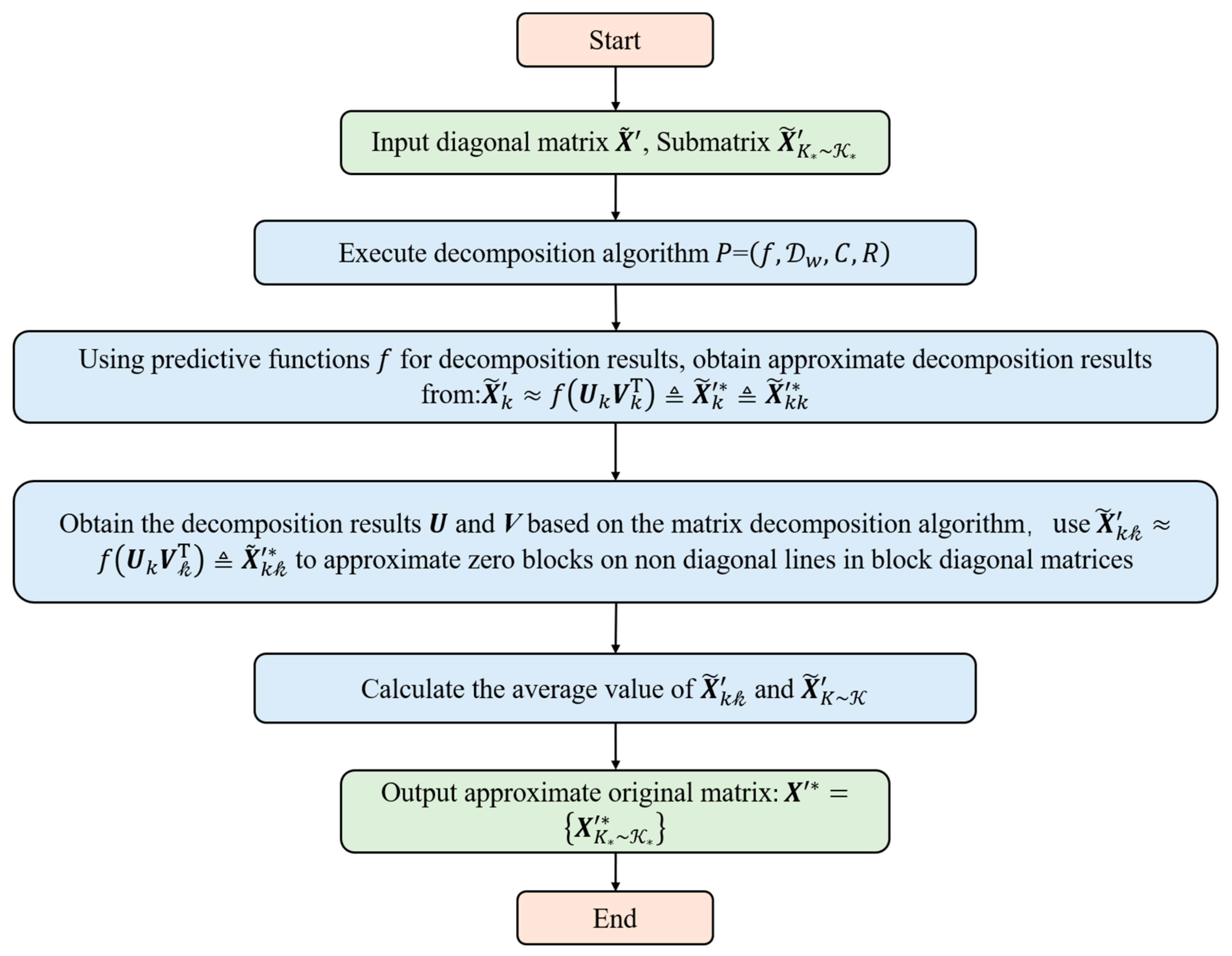
In the field of flood forecasting, since the matrices to be processed are usually sparse matrices and contain a large number of unobserved values, we usually set these unobserved values to 0. We designed a matrix decomposition method based on a diagonal block matrix. First, the original sparse matrix is iteratively transformed into a multi-layer two-sided block diagonal matrix, and then arranged into a block diagonal matrix, and the matrix decomposition algorithm is performed on the sub diagonal block matrix, and the original matrix through the decomposition results approximated. This can increase the density of the original matrix and alleviate the problems caused by data sparsity. The specific implementation process of this algorithm is shown in Figure 3:
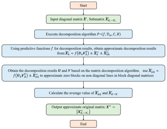
Figure 3.
Flowchart of matrix decomposition method based on diagonal block matrix.
Based on the above decomposition techniques, in the k-th mode, it is decomposed into sub-problems on matrix pairs , with the following optimization objectives:
where is a given incomplete matrix obtained from higher-order incomplete tensors through TT decomposition; is the incomplete binary matrix of , if is known, if is missing, and ; and ⊙ represents the Hadamard product, combining different pattern matrices together:
The EWLRTC-TT model formula is as follows, different from the fixed indicator matrix Mk in pattern k. EWLRTC-TT adopts the automatic update weight Wk of the k-th mode matrix, then the goal can be formulated as:
Wk no longer remains static at 0 and 1, instead using the estimation of missing positions wij ∈ (0, 1) to fill it, if element xij is known, wij = 1.
This article constructs a maximization objective function. Based on the research in [30], the optimal convex approximation tensor kernel norm can replace tensor rank. Combining the characteristics of tensor rank, the following optimization problem is obtained:
represents tensor kernel norms, αk represents the weight of X[k]; the matrix flattens along the k-th mode. Ω is a partial observation set with unknown noise, is the number of damaged objects with missing entries, 𝒵 is the recovery object, and norms are used to separate sparse components from observations. Generate adaptive weights based on the change in matrix rank of Equation (18) above, and add the norm term:
where , the first term of Equation (19) and comes from Equation (18), which is summarized and weighted α relevant information. Flat matrix The larger the kernel norm, the greater the weight forced to maintain more basic tensor data information. The new term in Equation (19) is the penalty term used to smoothen the weight distribution.
To ensure the identifiability of the solution, the norm penalty of and is introduced into the above formula.
Due to the use of norm penalty, we update the weight of the k-th mode through convex function. This function follows the equation used in:
where hyperparameter c and Ξ is a normal number. Therefore, by iteratively calculating and , we can guarantee the (local) optimal solution.
In order to deal with the identifiability of the permutation of the decomposition technique proposed in this paper, the r column vector is rearranged and we can get the following equation:
This is similar to applying a descending order of eigenvalues in matrix decomposition. The rearrangement of the column vector can be realized during or after the proposed algorithm, because it does not affect the estimation process.
2.2.3. Heterography Module
As shown in Figure 4, based on the definition of heterogeneous graph, it is necessary to divide the objects in the study basin into multiple tensor is proton graphs, and define multiple interaction relationships based on prior knowledge, as shown in Formula (23):
where r represents the connection relationship of objects in the heterogeneous graph module; f represents the characteristics of the object; y represents the estimated quantity; V′ represents the set of objects selected to estimate y. The node attention introduced in this module is used to measure the impact of different nodes on this node at a certain time. By comparing the similarity of the characteristics of the source node and the target node in the target space, the function weight of the adjacent nodes of the source node on the source node is given.

Figure 4.
Schematic diagram of attention-heterography module.
- Node attention module
As shown in Figure 5, the current status of the target node at a certain time is marked as , for its multiple adjacent nodes, its status is marked as , where represents one of all adjacent nodes of node j, and the state of the target node at the next time is affected by the state of all adjacent nodes at the current time.

Figure 5.
Schematic diagram of node attention module.
The node focus module maps the source node state and the target node state to the same space through the linear layer weights and , respectively. After the splicing operation, the initial node weight is calculated through the full connection layer weight , and then after the normalization and activation operation.
Obtain the final node weight . As shown in Equation (27), the single relationship state variable temporarily records the impact of all adjacent nodes on the state transition of the target node in the relationship r:
where ⊕ represents corresponding element addition operation, and ⊙ a represents Hadamard product operation.
- 2.
- Relational attention module
In the heterogeneous graph iteration module, there are usually multiple relationships between nodes, and the relationship attention weight is an important basis on which to measure the impact of different relationships on node status. As shown in Figure 6 below, in a single relationship, the impact of multiple nodes on the state of the target node is weighted by the node attention module and recorded as . The relational attention module processes the information incentives from all relationships at the current moment through the splicing operation and the linear layer, so as to obtain the weight of different relational signals .

Figure 6.
Schematic diagram of Relational attention module.
As shown in Formula (29), the initial relationship weight is obtained after initial linear change (), activation processing (tan h), and linear weighting operation ().
As shown in Formula (30), the final relational attention weight is obtained after softmax normalization .
- 3.
- Among these, represents the weight of the r-th relationship to node j.
In order to further improve the stability of the node attention module, this paper adopts the multi-dimension attention mechanism (MHAM):
that is, through multiple attention modules to carry out weighting operations, splice the features from multiple weighted processing to obtain the output results, and help the prediction model achieve better prediction results in the test set:
2.2.4. Temporal Feature Extraction
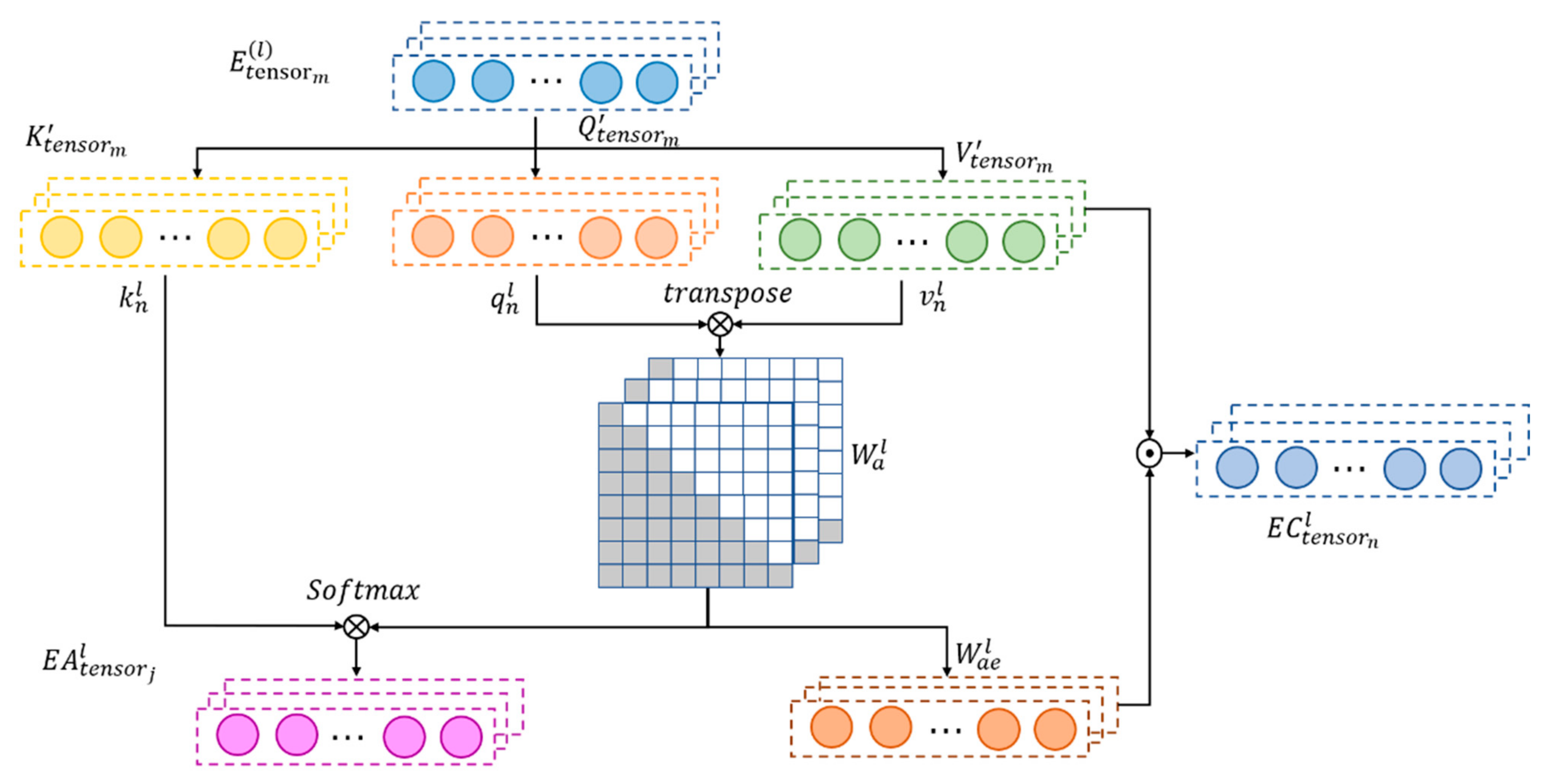
From the perspective of time, the data measured by the hydrological station at the current time and the data measured at different times in the past are time-dependent and will change with time. An attention mechanism can find more influential and relevant spatiotemporal features of the target object, so as to better mine temporal features. This section establishes an attention layer to process the output of the above spatiotemporal feature mining model, as shown in Figure 7 below.
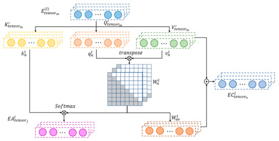
Figure 7.
Schematic of temporal attention module.
First, the spatiotemporal tensor is input, where m represents the sequence length and 1 represents the hidden layer of the first layer input, dilated convolutions with different kernel sizes as hidden layers across L layers. By stacking L layers of advanced causal dilated blocks across depth and time, a complete TCN-AM network is built and is called dilated convolution. Furthermore, dilated convolutions are used to give the network a sufficient receptive field, thus maintaining the computational efficiency of the network. The size of the dilation grows exponentially with the depth of the network ( for the l-th layer in the network).
The calculation steps of the temporal attention modules are defined as follows.
Step 1: Calculate the time self-attention importance of , where is an intermediate variable containing information before time step t. The temporal self-attention module utilizes the information of all-time steps, including past and future information of time step t. However, for time-series data, only past information can be processed; thus, the processing of weight matrix is refined to meet their sequence characteristics.
Step 2: In the first step, three linear transformations , are used to map to three different vectors of dimension , namely, , , and . The dot product of and is calculated and divided by to obtain the weight matrix , where . The lower triangular part of is extracted: , and the remaining part of the weight matrix is set to 0, which can mask the weight of future time steps, such that future information is not used. Finally, normalization is performed with softmax. is calculated as follows: , where , and t is the time step (t = 1,2, ⋯, m).
Step 3: A causal dilation convolution operation is performed on to obtain , where represents the output of causal convolution, and causal dilation blocks can be stacked into many layers. To ensure each layer is of the same length, zero padding is added to the left so that the input information on the left gradually accumulates to the right.
2.2.5. Model Train
To optimize the penalty objective function of the physical constraints we introduce, we adopt the maximum block improvement (MBI) algorithm [31], which has two advantages over the traditional cyclic block coordinate descent (BCD) algorithm. Firstly, it has good algorithm characteristics that can ensure convergence to a stable point. Secondly, under the tensor optimization model with spherical constraints, this method has strong convergence. When choosing spatiotemporal features as tensor patterns, the eigenvalues of flood data and influencing factors are different at different times, and the eigenvalues of influencing factors can be regarded as additional tensor patterns of higher-order tensors. However, higher-order tensors require more complex and intensive calculations, and in general practice, we assume that the order of the tensor and the number of influencing factors can be determined based on prior knowledge. In the tensor pre-processing stage, appropriate correlations are given γ and λ, a group of partially observed damaged entries Ω, with a structure similar to , where is low-rank and is sparse, and can be optimized through two steps. The optimized external framework is BCD, which is used to update parameters α and . The internal framework is alternating direction method of multipliers (ADMM), used to optimize due to the internal framework problem caused by the inherent correlation between and can be solved for specific algorithms.
3. Results
The purpose of this section is to show the execution details and experimental results. The data set describes the data set of Qijiang Basin used. The baseline and implementation settings display baseline, model structure, and parameter information. The evaluation indicators list two commonly used evaluation indicators and two interval prediction indicators.
3.1. Datasets
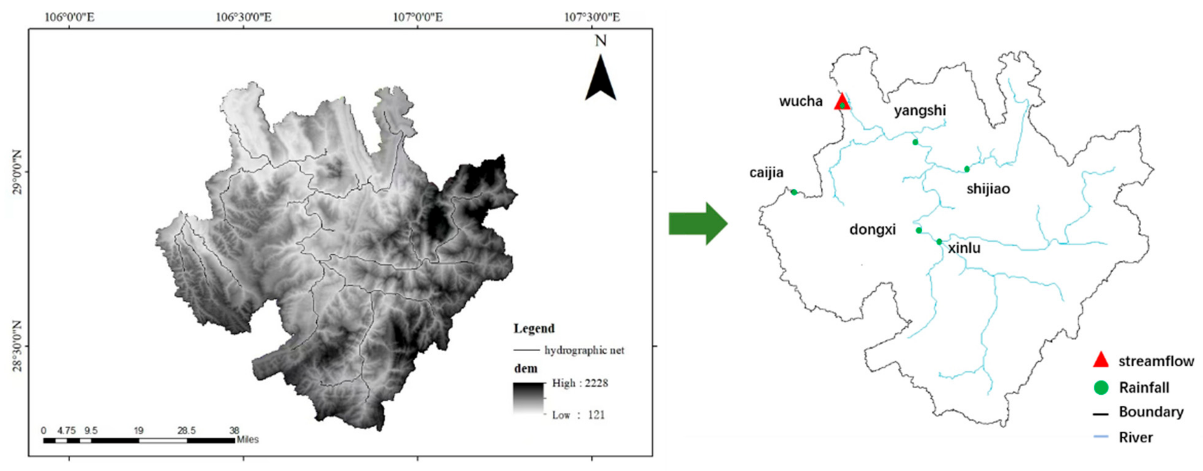
In order to better compare the performance of the proposed method and baseline model, the Qijiang Basin in Chongqing, China was selected as the experimental target basin, and relevant measurement data from the Qijiang Basin in Chongqing were used for the experiment. The flow data used in the experimental watershed come from hydrological stations within the watershed, including six rainfall stations (Wucha, Caijia, Shijiao, Xinlu, Dongxi, and Yangshi) and one flow station (Wucha). Figure 7 shows the distribution of stations in the experimental watershed. From the graph, it can be seen that there is a certain spatial correlation between the upstream and downstream stations in the watershed. The meteorological data used in the experiment were from mobile phones and the National Meteorological Information Center of China. Specific types of meteorological data include evaporation data, rainfall data, temperature data, and wind speed data. The input for the experiment includes previous data from 1 to 12 days (including the current). The output is runoff data for the next 1–6 days. The time span of the Qijiang River Basin dataset is from 1 January 1979 to 31 December 2020. The data granularity is one item per day. Due to the fact that the above data usually follow a relatively clear data distribution, in order to better partition the dataset while maintaining the data distribution, this study used a random shuffling method to shuffle the original dataset to approximate the random distribution. Then, through linear partitioning, the original dataset is divided into training, validation, and testing sets in different proportions.
3.2. Baseline and Parameter Settings
We compare the DK-HTAN with one machine learning method, two non-attention based neural network methods, and two attention-based methods:
SVR [32]: Support vector regression. A simple and robust machine learning network, the basic idea is to find a regression plane so that all points are closest to the plane.
RNN: Convolution neural network. The RNN model is mainly composed of three type of layer: input layer, output layer, and hidden layer.
LSTM: Long short-term memory network, a variant of RNN, adopts gating mechanism and optimizes the network of RNN.
STALSTM [33]: The STALSTM model adds attention modular to the original LSTM model. Similarly to LSTM, the primary architecture and parameters are used.
AGCLSTM [34]: A novel graph convolution-based spatiotemporal attention LSTM (AGCLSTM) network to tackle the time-series prediction problem of flood forecasting.
DK-HTAN: The DK-HTAN model adds spatiotemporal attention module and an output interval prediction constructed by error factors on the basis of the original HCN model and TCN. The main architecture and parameters are the same as HCN and TCN.
Parameter settings: Experiments using Linux service platform (CPU: Intel (R) Xeon (R) CPU E5-2630) v4 @ 2.20 GHz, graphics processor NVIDIA GeForce TITAN Xp, 12GB, operating system Ubuntu 16.04, deep learning library Python, programming language Python 3.6) completed. For all datasets, 80% are used for training and 20% for testing. We trained the model to adjust the super parameters, such as the learning rate LR = 0.001, and the training batch size was set to 256.
3.3. Evaluation Metrics
The LUBE interval prediction method is used to make up for the inaccuracy of point prediction. It considers the prediction error caused by uncertain factors and obtains the upper and lower bounds under a given confidence level, providing effective information for decision makers. Therefore, this paper explores the effect of combining LUBE with a neural network in precipitation interval prediction. The influence of interval prediction can frequently be estimated from two facets, named the PI coverage probability (PICP) and PI normalized root-mean-square bandwidth (PINRW).
In addition to the index of interval prediction, we also use root-mean-square error (RMSE) and mean absolute percentage error (MAPE) as evaluation indicators. The evaluation indicators of RMSE and MAPE are defined as follows:
where is the predicted value, and represents the value of real runoff observation data.
3.4. Experimental Results
3.4.1. Comparison
To further corroborate the advantages of the model proposed in this research, the graphical representation in Figure 8 is used to show the PI quality of the six models contrasted. The contrast of PICP, PINRW and TIME of all models is as follows. The SVR model is the basic machine learning prediction model. By confronting the proposed model with baseline models, we discovered that both the PICP and PINRW indices are exceeded by the suggested model. Since PINRW and PICP are two opposing objects, the optimal solution chosen must have a PICP that is hardly more than 90% in order to ensure that its PINRW index is low. Due to the seasonality of flood data, we divided the data into flood season and non-flood season for experiments.
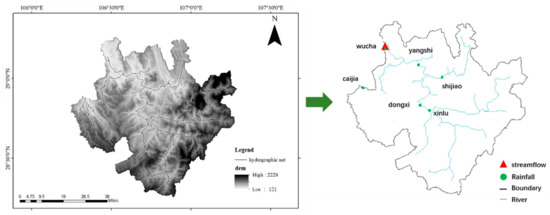
Figure 8.
Station distribution map of Qijiang River Basin.
ANN models of fusion tensor decomposition are instrumented to further verify the high PI quality of the proposed model. Table 1 shows that RNN, LSTM, STALSTM, AGCLSTM and the proposed model are at the same extent in terms of PICP, while the proposed model has a scarcely higher PICP index. Compared to the STALSTM and AGCLSTM models with spatiotemporal characteristics, it is improved 7.49% and 11.33% on the PICP index, respectively. The tensor decomposition method is used for the interpolation of the model preprocessing and the error factor adjustment part of the final output result to solve the nonlinear and nonstationary characteristics of the data, and the PI of DK-HTAN model is significantly smaller than RNN, LSTM, STALSTM, AGCLSTM. Therefore, it can be concluded that DK-HTAN is more suitable for solving the interval stacking problem caused by tensor decomposition. In the index of PINRW, DK-HTAN is improved by 4.08% and 11.26% over the AGCLSTM and STALSTM models.

Table 1.
Performance display data of the model under various interval prediction indicators.
Compared to the STALSTM and AGCLSTM models with spatiotemporal characteristics, DK-HTAN is improved by 5.88% and 13.18% on the MAPE index, respectively. Please refer to the data in Table 2 below. Furthermore, the method of using MBI to train the point prediction model and forming prediction intervals according to forecast error is faster than the method of using a meta-heuristic algorithm to train an interval prediction model. Generally speaking, the steady enhancement of PI quality is at the consumption of time. In the index of RMSE, DK-HTAN is improved by 17.84% and 21.90% over AGCLSTM and STALSTM models.

Table 2.
Performance display data of the model under MAPE and RMSE indicators.
3.4.2. Robustness Analysis
The model based on a data-driven and knowledge-guided framework effectively utilizes prior information and domain knowledge. In theory, it has stronger feature extraction ability and lower training data requirements for flood time-series data compared to pure data-driven flood prediction models. In this section, we analyzed the performance of data-driven and knowledge-guided flood prediction models and flood prediction ANN models under different boundary conditions and observations through comparative experiments. Specifically, we evaluated the performance and robustness of different models under different noise levels and outlier ratios.
Table 3 shows the impact of different noise levels on observation results compared to model predictions under different scales of noise. The noise gradually increased from 5% to 20%. Firstly, we can see that under different noise levels, DK has better PICP values compared to other models. This explains the performance advantages of the proposed model in interval prediction. Taking the Qijiang River Basin as an example, the PICP value of DK is about 15% higher than the dominant STALSTM. This may be because the model proposed in this article is based on data-driven and knowledge-guided design, and has strong robustness in the field of hydrological prediction. Of course, as the noise level increases, the interval performance of DK also shows a gradual convergence trend, which is also where we need further research and improvement. On the other hand, even if the noise level increases to 20%, the PICP performance of DK will not decrease much, which reflects the noise robustness of the model proposed in this paper with the help of data-driven and knowledge-guided techniques. Generally speaking, flood time-series data in practical engineering usually contain noise-interference data. It is difficult to distinguish useful data from interference values based on a single data-driven model. However, the dual driving mechanism proposed in this paper can effectively filter interference values using flood physical constraints, thereby improving the noise robustness of the DK model.

Table 3.
PICP performance of various models under different proportions of noisy data.
For the comparison of different models in flood time series data prediction, Outlier usually have a greater impact on the prediction results than noise. Therefore, here we compare the PICP performance of different models under different outliers. As shown in Table 4, the performance comparison of DK under different outlier ratios guided by flood prediction and physical constraint theory is shown in Table 5. The PICP value of DK proposed in this paper is higher than that of other baseline models under various outliers. Taking the Qijiang River Basin as an example, the PICP value of DK is 14%–28% higher than that of STALSTM. This may be because the data preprocessing method of tensor factor decomposition is adopted in this paper, which reduces the impact of outliers on the prediction accuracy of the model. The robustness of the model to outliers is improved. However, it should be noted that when the proportion of outliers is high, the PICP performance of DK also shows a trend of weakening. This may be because the input matrix of the model deviates from the normal range with the increase in outliers, leading to the decline of the prediction performance of the model.

Table 4.
PICP performance of each model under different proportions of outlier data.

Table 5.
Corresponding DK-HTAN model type table.
3.4.3. Attention Module Analysis of DK-HTAN
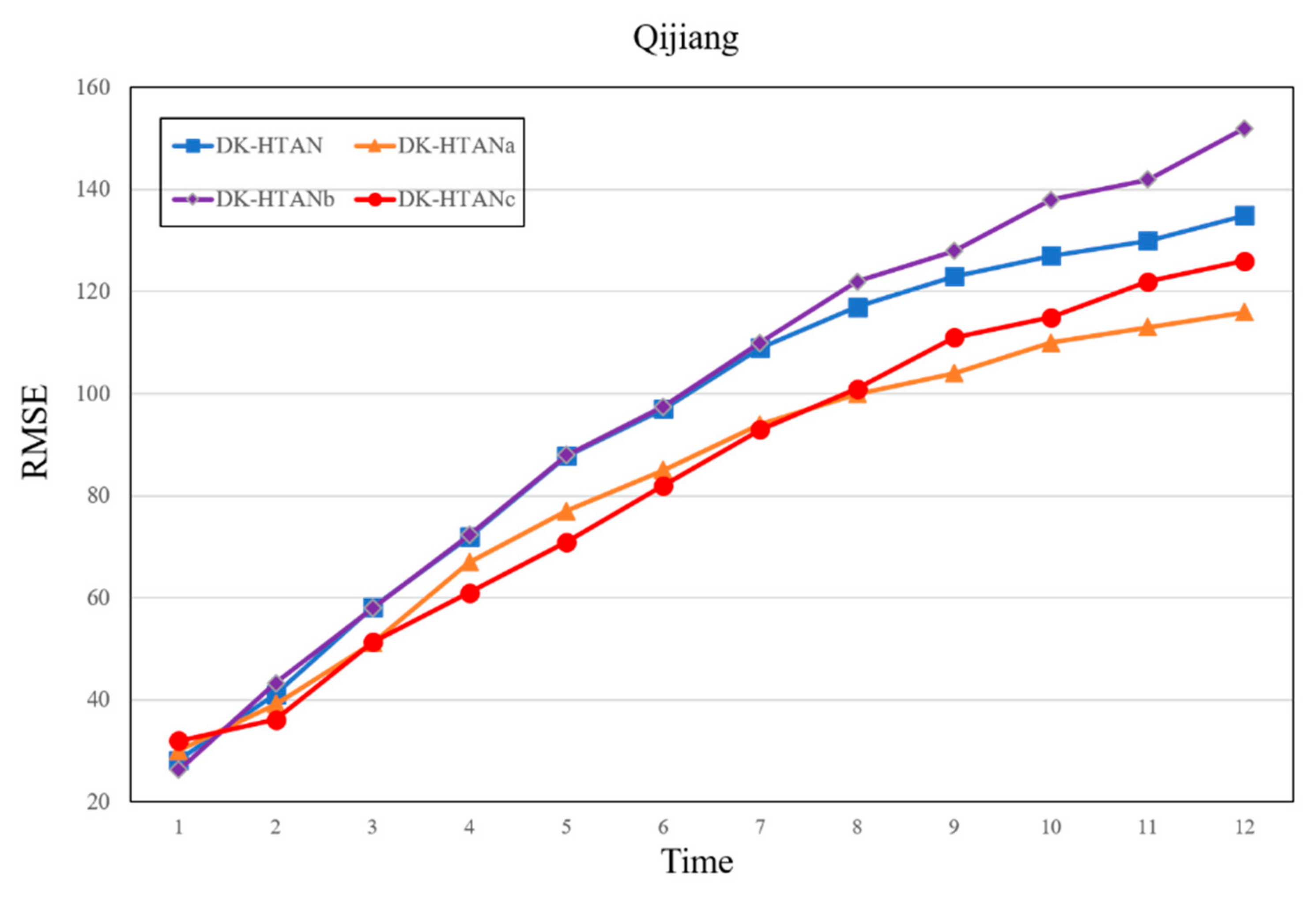
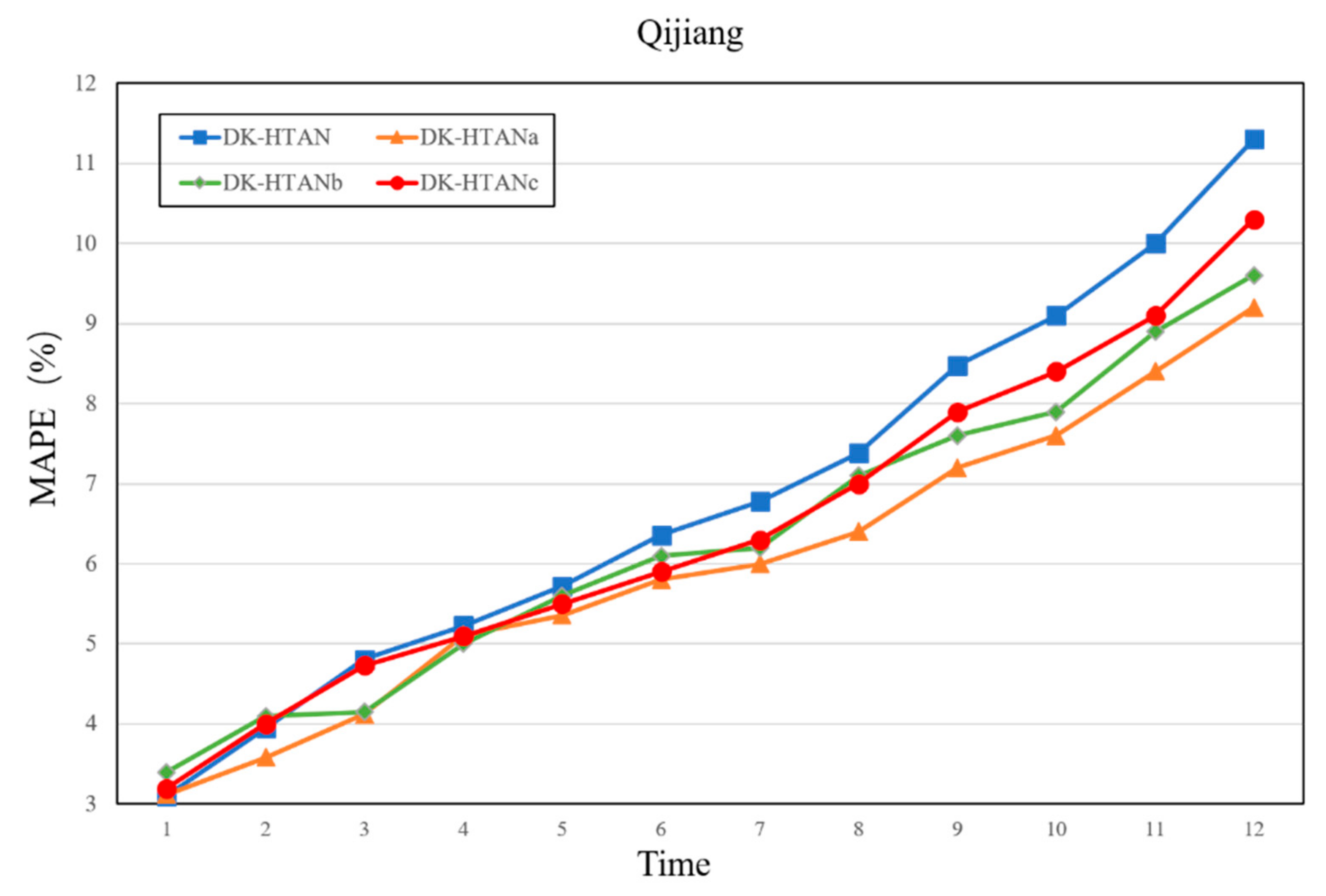
In the structure of the DK-HTAN model, the types of node attention modules and relational attention modules play an important role in the performance of the model. This part of the experiment discusses the performance of node attention types and relationship attention types on DK-HTAN model data in the Qijiang River Basin, in which node attention module types and types of relational attention modules include mean and weighted attention.
Figure 9 and Figure 10 show the performance impact of different attention-type combinations on the DK-HTAN model. On the Qijiang Basin dataset, the overall performance of different models is similar. However, the type of attention model has a certain impact. The performance of the weighted model is in the middle, although intuitively, the model using DK-HTAN with weighted attention should perform better than the model using only average attention modules. However, in this experiment, the experimental results are different from the expected assumptions: the mean-type relational attention module can enhance the performance of the model more, and the weighted-type node attention module can enhance the outcomes of the model more. In general, weighted attention has a positive effect on model performance, while average attention has a stabilizing effect on model performance. However, due to the error characteristics of neural network model training, the training quality has a certain impact on the performance of the weighted attention module. If the training quality of the weighted focus module is not enough, the performance of the model may not be improved. At the same time, considering that the most important prior relationship has been put into the model when modeling, its mean relational attention module can better reflect the performance of the model. Although in this part of the experiment, the weighted focus method did not always maintain its advantages, it still showed good performance. At the same time, the overall performance of the DK-HTAN model surpassed other baseline models and other defined models.
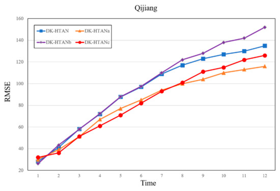
Figure 9.
RMSE performance of different attention combinations.

Figure 10.
MAPE performance of different attention combinations.
4. Discussion
Through experiments, it was found that the proposed model outperforms the baseline model in all indicators, indicating that our model has superior performance. This may be the result of the internal structural characteristics of tensors, which make data input better into the model for processing. In addition, the model adds a heterogeneous graph attention module, which increases the prior knowledge of the model and better optimizes the initial conditions. The time-series prediction module uses TCN, greatly reducing training costs. Finally, optimize and adjust the model using physical constraints to make the predicted results more in line with physical mechanisms. Although dual driving enhances the learning ability of the model and effectively utilizes prior knowledge and domain-specific information in this case, it only embeds a control equation and the neural network output only contains one variable, which may affect prediction accuracy. Future research can include multi-constraint, high-dimensional flood forecasting scenarios.
5. Conclusions
In order to process massive flood data with rich spatiotemporal characteristics, we propose a flood interval prediction method based on data-driven and knowledge-guided heterogeneous graphs and time convolutional networks (DK-HTAN). Experiments on the Qijiang dataset show that the prediction accuracy of the proposed model is significantly better than the bassline models—11.4% on the PICP index. The combination of physical constraint guidance and deep learning methods in this article is a preliminary attempt to apply a knowledge- and data-driven approach to flood prediction. In addition, more external factors, including watershed vegetation and human settlements, need to be used in future work. Inspired by the generative adversarial network (GAN) model, our next paper will consider further enhancing flood prediction through reverse generation and distribution of watershed data.
Author Contributions
Conceptualization, J.F.; methodology, P.S. and J.F.; validation, J.L. and P.S.; formal analysis, W.W.; investigation, W.W.; writing—original draft preparation, P.S.; writing—review and editing, P.S. and J.F.; visualization, Y.W.; supervision, Y.W.; project administration, J.F.; funding acquisition, J.F. All authors have read and agreed to the published version of the manuscript.
Funding
This work was supported in part by the following projects: The National Key R&D Program of China (grant 2021YFB3900601), Water Conservancy Science and Technology Program of Jiangsu (grant 2022002), and Major Science and Technology Program of the Ministry of Water Resources (grant SKS-2022132). Funder: Jun Feng.
Institutional Review Board Statement
The studies not involving humans or animals.
Informed Consent Statement
The study did not involve humans or animals.
Data Availability Statement
No new data were created or analyzed in this study. Data sharing is not applicable to this article.
Conflicts of Interest
The authors declare no conflict of interest.
References
- Shi, Y.; Yao, Q.; Wen, J.; Xi, J.; Li, H.; Wang, Q. A spatial accessibility assessment of urban tourist attractions emergency response in Shanghai. Int. J. Disaster Risk Reduct. 2022, 74, 102919. [Google Scholar] [CrossRef]
- Yang, H.; Li, W. Data decomposition, seasonal adjustment method and machine learning combined for runoff prediction: A case study. Water Resour. Manag. 2023, 37, 557–581. [Google Scholar] [CrossRef]
- Li, K.; Huang, G.; Wang, S.; Razavi, S. Development of a physics-informed data-driven model for gaining insights into hydrological processes in irrigated watersheds. J. Hydrol. 2022, 613, 128323. [Google Scholar] [CrossRef]
- Wu, C.; Zhang, X.; Wang, W.; Lu, C.; Zhang, Y.; Qin, W.; Shu, L.; Tick, G.R.; Liu, B. Groundwater level modeling framework by combining the wavelet transform with a long short-term memory data-driven model. Sci. Total Environ. 2021, 783, 146948. [Google Scholar] [CrossRef] [PubMed]
- He, X.; Liu, R.; Anumba, C.J. Data-driven insights on the knowledge gaps of conceptual cost estimation modeling. J. Constr. Eng. Manag. 2021, 147, 04020165. [Google Scholar] [CrossRef]
- Xia, M.; Shao, H.; Ma, X.; de Silva, C.W. A stacked GRU-RNN-based approach for predicting renewable energy and electricity load for smart grid operation. IEEE Trans. Ind. Inform. 2021, 17, 7050–7059. [Google Scholar] [CrossRef]
- Wang, H.; Lu, B.; Li, J.; Liu, T.; Xing, Y.; Lv, C.; Hashemi, E.; Cao, D.; Li, J.; Zhang, J. Risk Assessment and Mitigation in Local Path Planning for Autonomous Vehicles With LSTM Based Predictive Model. IEEE Trans. Autom. Sci. Eng. 2021, 19, 2738–2749. [Google Scholar] [CrossRef]
- Cao, X.; Ren, N.; Tian, G.; Fan, Y.; Duan, Q. A three-dimensional prediction method of dissolved oxygen in pond culture based on Attention-GRU-GBRT. Comput. Electron. Agric. 2021, 181, 105955. [Google Scholar] [CrossRef]
- Wang, Q.; Huang, K.; Chandak, P.; Zitnik, M.; Gehlenborg, N. Extending the nested model for user-centric XAI: A design study on GNN-based drug repurposing. IEEE Trans. Vis. Comput. Graph. 2022, 29, 1266–1276. [Google Scholar] [CrossRef]
- Pradhyumna, P.; Shreya, G.P. Graph neural network (GNN) in image and video understanding using deep learning for computer vision applications. In Proceedings of the 2021 Second International Conference on Electronics and Sustainable Communication Systems (ICESC), Coimbatore, India, 4–6 August 2021; pp. 1183–1189. [Google Scholar]
- Yang, Z.; Dong, S. HAGERec: Hierarchical attention graph convolutional network incorporating knowledge graph for explainable recommendation. Knowl.-Based Syst. 2020, 204, 106194. [Google Scholar] [CrossRef]
- Wang, T.; Jin, D.; Wang, R.; He, D.; Huang, Y. Powerful graph convolutional networks with adaptive propagation mechanism for homophily and heterophily. In Proceedings of the 36th AAAI Conference on Artificial Intelligence, Virtual, 22 February–1 March 2022; Volume 36, pp. 4210–4218. [Google Scholar]
- Gupta, K.; Ajanthan, T. Improved gradient-based adversarial attacks for quantized networks. In Proceedings of the 36th AAAI Conference on Artificial Intelligence, Virtual, 22 February–1 March 2022; Volume 36, pp. 6810–6818. [Google Scholar]
- Lindemann, B.; Müller, T.; Vietz, H.; Jazdi, N.; Weyrich, M. A survey on long short-term memory networks for time series prediction. Procedia CIRP 2021, 99, 650–655. [Google Scholar] [CrossRef]
- Fan, J.; Zhang, K.; Huang, Y.; Zhu, Y.; Chen, B. Parallel spatio-temporal attention-based TCN for multivariate time series prediction. Neural Comput. Appl. 2023, 35, 13109–13118. [Google Scholar] [CrossRef]
- Zhou, M.; Wang, B.; Guo, S.; Watada, J. Multi-objective prediction intervals for wind power forecast based on deep neural networks. Inf. Sci. 2021, 550, 207–220. [Google Scholar] [CrossRef]
- Peng, X.; Wang, H.; Lang, J.; Li, W.; Xu, Q.; Zhang, Z.; Li, C.; Cai, T.; Duan, S.; Liu, F. EALSTM-QR: Interval wind-power prediction model based on numerical weather prediction and deep learning. Energy 2021, 220, 119692. [Google Scholar] [CrossRef]
- Piadeh, F.; Behzadian, K.; Alani, A.M. A critical review of real-time modelling of flood forecasting in urban drainage systems. J. Hydrol. 2022, 607, 127476. [Google Scholar] [CrossRef]
- Deutz, S.; Bardow, A. Life-cycle assessment of an industrial direct air capture process based on temperature–vacuum swing adsorption. Nat. Energy 2021, 6, 203–213. [Google Scholar] [CrossRef]
- Wei, Q.; Li, X.; Song, M. De-aliased seismic data interpolation using conditional Wasserstein generative adversarial networks. Comput. Geosci. 2021, 154, 104801. [Google Scholar] [CrossRef]
- Chen, X.; Wang, J.; Zhang, G.; Peng, Q. Tensor-Based Parametric Spectrum Cartography From Irregular Off-Grid Samplings. IEEE Signal Process. Lett. 2023, 30, 513–517. [Google Scholar] [CrossRef]
- Chen, X.; He, Z.; Wang, J. Spatial-temporal traffic speed patterns discovery and incomplete data recovery via SVD-combined tensor decomposition. Transp. Res. Part C Emerg. Technol. 2018, 86, 59–77. [Google Scholar] [CrossRef]
- Zhou, S.; Erfani, S.; Bailey, J. Online CP decomposition for sparse tensors. In Proceedings of the 2018 IEEE International Conference on Data Mining (ICDM), Singapore, 17–20 November 2018; pp. 1458–1463. [Google Scholar]
- Che, M.; Wei, Y. Randomized algorithms for the approximations of Tucker and the tensor train decompositions. Adv. Comput. Math. 2019, 45, 395–428. [Google Scholar] [CrossRef]
- Yuan, L.; Li, C.; Mandic, D.; Cao, J.; Zhao, Q. Tensor ring decomposition with rank minimization on latent space: An efficient approach for tensor completion. In Proceedings of the AAAI Conference on Artificial Intelligence, Honolulu, HI, USA, 27 January–1 February 2019; Volume 33, pp. 9151–9158. [Google Scholar]
- Wang, J.; Xu, G.; Li, C.; Wang, Z.; Yan, F. Surface defects detection using non-convex total variation regularized RPCA with kernelization. IEEE Trans. Instrum. Meas. 2021, 70, 1–13. [Google Scholar] [CrossRef]
- He, X.; Deng, K.; Wang, X.; Li, Y.; Zhang, Y.; Wang, M. Lightgcn: Simplifying and powering graph convolution network for recommendation. In Proceedings of the 43rd International ACM SIGIR Conference on Research and Development in Information Retrieval, Virtual, 25–30 July 2020; pp. 639–648. [Google Scholar]
- Hewage, P.; Behera, A.; Trovati, M.; Pereira, E.; Ghahremani, M.; Palmieri, F.; Liu, Y. Temporal convolutional neural (TCN) network for an effective weather forecasting using time-series data from the local weather station. Soft Comput. 2020, 24, 16453–16482. [Google Scholar] [CrossRef]
- Yang, J.H.; Zhao, X.L.; Ji, T.Y.; Ma, T.H.; Huang, T.Z. Low-rank tensor train for tensor robust principal component analysis. Appl. Math. Comput. 2020, 367, 124783. [Google Scholar] [CrossRef]
- Kong, X.; Yang, C.; Cao, S.; Li, C.; Peng, Z. Infrared small target detection via nonconvex tensor fibered rank approximation. IEEE Trans. Geosci. Remote Sens. 2021, 60, 5000321. [Google Scholar] [CrossRef]
- Chen, Z.; Liang, J.; Wang, T.; Tang, B.; So, H.C. Generalized MBI algorithm for designing sequence set and mismatched filter bank with ambiguity function constraints. IEEE Trans. Signal Process. 2022, 70, 2918–2933. [Google Scholar] [CrossRef]
- Dodangeh, E.; Panahi, M.; Rezaie, F.; Lee, S.; Bui, D.T.; Lee, C.W.; Pradhan, B. Novel hybrid intelligence models for flood-susceptibility prediction: Meta optimization of the GMDH and SVR models with the genetic algorithm and harmony search. J. Hydrol. 2020, 590, 125423. [Google Scholar] [CrossRef]
- Ding, Y.; Zhu, Y.; Wu, Y.; Jun, F.; Cheng, Z. Spatio-temporal attention LSTM model for flood forecasting. In Proceedings of the 2019 International Conference on Internet of Things (IThings) and IEEE Green Computing and Communications (GreenCom) and IEEE Cyber, Physical and Social Computing (CPSCom) and IEEE Smart Data (SmartData), Atlanta, GA, USA, 14–17 July 2019; pp. 458–465. [Google Scholar]
- Yan, L.; Feng, J.; Hang, T.; Zhu, Y. Flow interval prediction based on deep residual network and lower and upper boundary estimation method. Appl. Soft Comput. 2021, 104, 107228. [Google Scholar] [CrossRef]
Disclaimer/Publisher’s Note: The statements, opinions and data contained in all publications are solely those of the individual author(s) and contributor(s) and not of MDPI and/or the editor(s). MDPI and/or the editor(s) disclaim responsibility for any injury to people or property resulting from any ideas, methods, instructions or products referred to in the content. |
© 2023 by the authors. Licensee MDPI, Basel, Switzerland. This article is an open access article distributed under the terms and conditions of the Creative Commons Attribution (CC BY) license (https://creativecommons.org/licenses/by/4.0/).

