Pore Water Pressure Prediction Based on Machine Learning Methods—Application to an Earth Dam Case

Featured Application

This work is intended to provide additional approaches for analyzing and interpreting dam monitoring data.

Abstract

Pore water pressure (PWP) response is significant for evaluating the earth dams’ stability, and PWPs are, therefore, generally monitored. However, due to the soil heterogeneity and its non-linear behavior within earths, the PWP is usually difficult to estimate and predict accurately in order to detect a pathology or anomaly in the behavior of an embankment dam. This study endeavors to tackle this challenge through the application of diverse machine learning (ML) techniques in estimating the PWP within an existing earth dam. The methods employed include random forest (RF) combined with simulated annealing (SA), multilayer perceptron (MLP), standard recurrent neural networks (RNNs), and gated recurrent unit (GRU). The prediction capability of these techniques was gauged using metrics such as the coefficient of determination (R²), mean square error (MSE), and CPU training time. It was found that all the considered ML methods could give satisfactory results for the PWP estimation. Upon comparing these methods within the case study, the findings suggest that, in this study, multilayer perceptron (MLP) gives the most accurate PWP prediction, achieving the highest coefficient of determination (R² = 0.99) and the lowest mean square error (MSE = 0.0087) metrics. A sensitivity analysis is then presented to evaluate the models’ robustness and the hyperparameter’s influence on the performance of the prediction model.

1. Introduction

Dam structure health monitoring plays a crucial role in the dam’s safety. The primary goal is to gather data concerning the assessment of an earth dam throughout its entire lifespan. One of the important monitoring parameters in earth dams is pore water pressure (PWP). It can be obtained by piezometers (PWP cells) installed in the earths. A proper evaluation of PWP helps to monitor the behavior after construction and indicates potentially dangerous conditions that may adversely affect the structure stability [1,2]. Inversely, PWP is a prediction factor for damages that can occur in earth dams. Rationally predicting the PWP could be an effective indicator for evaluating the safety of earth dams. Monitoring PWP is particularly important for an embankment dam. On the one hand, an excessive increase in PWP can lead to dam failure through slope failure. On the other hand, monitoring variations in PWP makes it possible to detect a pathology or anomaly in the behavior of the dam. For example, an increase in PWP that is not explained by a cyclic/reversible variation in the level of the reservoir or the season could be associated with a pathology, such as the clogging of the drainage system or the initiation of an internal erosion process.

Initially, PWP prediction models were developed based on the fundamental laws of fluid mechanics in porous media [3]. Analytical solutions [4,5], numerical simulations [6,7,8], statistic models [9,10], and probabilistic models [11,12] have been developed to obtain the PWP by applying these different methodologies. In practical engineering, due to inhomogeneous and highly non-linear phenomena in earth soils, these models could not accurately evaluate the hydraulic behavior by comparing the provided results with the in situ measurements.

The trend toward automating dam monitoring devices is gaining momentum, enabling higher reading frequencies and an abundance of monitoring data [13]. Within the machine learning (ML) community, sophisticated tools have been developed for constructing data-driven prediction models in geotechnical engineering [14,15] such as to evaluate soil properties [16], investigate the reliability of excavations [17,18,19], analyze the deformations [20,21] and ground settlement [22], as well as predict geotechnical parameters [23]. The significant advantage of the ML methods is that they can fit highly non-linear behaviors. This is a key factor in their current popularity.

There are several recent works available in the literature on the use of machine learning methods for the analysis of dam monitoring measurements. More specifically, [13,24,25,26] are interested in modeling displacement measurements of arch dams; [27,28] focus on displacements of gravity and buttress dams; [9,29] deal with pore pressures at the base of arch dams, and [30] concern settlements of embankment dams.

Advancements have been made in utilizing machine learning (ML) techniques for predicting pore water pressure (PWP) in diverse geotechnical fields like slope stability. Mustafa et al. (2013) [31] investigated the effectiveness of different training algorithms within ANN for PWP prediction. Their study highlighted the Levenberg Marquardt (LM) algorithm as particularly efficient and rapid in modeling the dynamics of soil pore water pressure changes in response to rainfall patterns. Mohammed proposed a “grey model” that integrates the finite element method (FEM) with the ANNs [32], aiming for a more accurate forecast of PWP variations. Tayfur et al. (2005) [33] conducted a comparative analysis between FEM and ANNs for flow seepage through the Jeziorsko earth-fill dam in Poland. Their discussion touched upon the suitability and competitiveness of ANNs against FEM in predicting seepage through the dam. Wei et al. [3] showcased the enhanced precision and robustness of gated recurrent unit (GRU) and Long Short-Term Memory (LSTM) models in predicting slope seepage/stability under rainfall compared to the standard RNNs. RF has been applied to the prediction of daily pore water pressure in the embankment [34,35], and MLP has been used in the case of concrete dam seepage behavior [9]. RNNs and GRU are applied in pore water pressure prediction of a tunnel boring machine [36] and slope [3]. These elements have been added to the end of the introduction section for each method.

In the previous studies mentioned above, most of the research was limited to the ANN method but not various ML methods for predicting PWP in earth dams. Moreover, these studies did not discuss the time effect and irreversible effect, which are important factors in the safety of earth dams.

This paper deals with the use and comparison of several machine learning methods for analyzing monitoring data and predicting PWP in earth dams. This type of approach can be useful for detecting pathology or abnormal dam behavior.

The aim of this study is to forecast PWP in embankment dams using several ML techniques, such as random forest (RF) with simulated annealing (SA), multilayer perceptrons (MLP), traditional recurrent neural networks (RNNs), and gated recurrent unit (GRU). This research marks the initial effort to use diverse static and dynamic neural networks to analyze monitoring data and to compare their accuracy in predicting the evolution of PWP in earth dams. The case study of this paper is a 36 m high earth dam. It is equipped with 45 piezometers (PWP cells), and four represented sensors monitoring data are chosen to build and validate the prediction models. Prediction models show the powerful capacity to predict PWP, which could make a reference for applying ML methods in non-linear and time series hydraulic problems in geotechnics.

2. Materials and Methods

ML methods can be classified into supervised or unsupervised techniques based on the availability of a training dataset. Supervised ML is designed to generate desired outputs in response to a given set of inputs during training. This technique is commonly employed for modeling and controlling dynamic systems, classifying noisy data, and making predictions about future events. On the other hand, unsupervised ML is trained in a manner where the network continuously adapts to novel inputs. It has the ability to reveal non-linear relationships within the data and establish classification schemes that adjust to variations in the added data. In this study, supervised ML techniques are utilized. There are 4 kinds of supervised ML techniques selected to explore the best suitable methods for predicting time-series database, i.e., PWP.

Most deep learning methods are good at training time series datasets; two kinds of them are chosen in this study, including RNNs and GRU. RNNs are neural networks suitable for processing sequence data that can effectively capture the temporal information in the sequence. RNNs use the same parameters at each time step, which can effectively share weights and reduce the complexity of the model and the number of parameters for training. RNNs can memorize previous information and use it to make predictions or decisions in subsequent time steps, which is very useful for handling context-dependent tasks. The disadvantage of RNNs is that they often yield vanishing gradients and gradient explosions during training.

In order to avoid the drawbacks of RNNs, GRU has been employed in this study. GRU has a simpler structure compared to LSTM, solves the problem of vanishing gradients compared to RNNs, and has been shown to be more effective for smaller sequences.

Deep learning suffers from a uniform common problem, i.e., training is inefficient, time-consuming, and computationally demanding. In order to compare the computation time and find the most accurate and efficient training method for the case of this paper, the two most commonly used ML methods, RF and MLP, are selected for this paper.

2.1. Random Forests Combined with Simulated Annealing

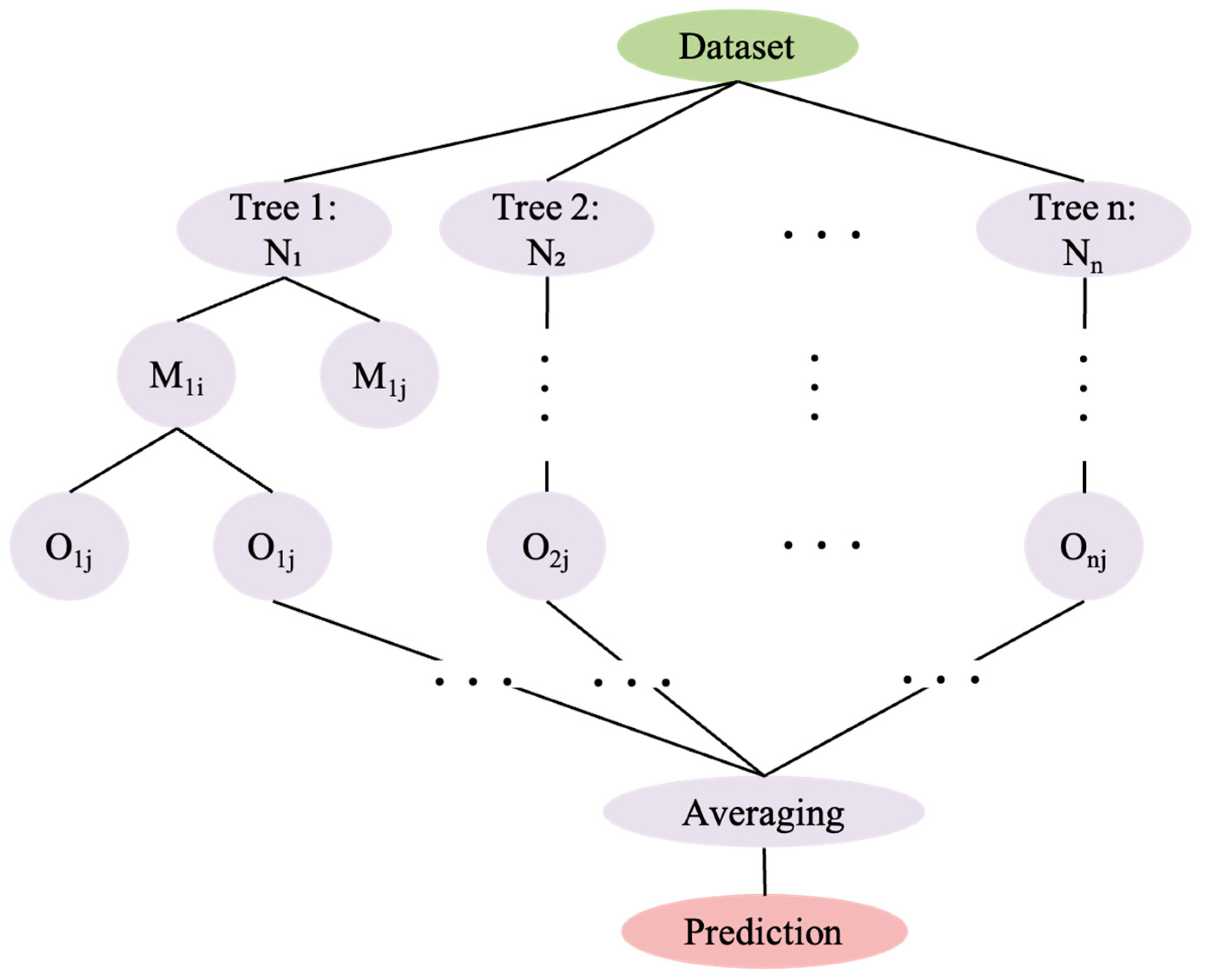
2.1.1. Random Forest

Random forest (RF) is an ML technique that groups decision trees for tasks such as classification or regression. In a random forest, each single tree makes a class prediction, and the class with the most calls is chosen as the model’s prediction. The architecture of an RF for regression is established through the four steps [37] stated below and shown in Figure 1.

Step 1: Generate a dataset with a sample size of N by replacement. Utilize these selected N samples to train a decision tree, which serves as the sub-sample at the root node of the tree;

Step 2: At each node of the decision tree, randomly pick m attributes from the total M attributes of each sample, where m is considerably smaller than M. Next, employ a specific tactic, such as information gain, from these m attributes to choose one attribute as the splitting attribute for the node;

Step 3: Throughout the decision tree’s construction, each node must undergo splitting as described in step 2 until it reaches a point where further division is not possible;

Step 4: repeat steps 1 to 3 to generate a random forest with a significant number of decision trees.

Since its introduction by Breiman [37], RF has become a highly popular method for establishing prediction models. The RF model offers several advantages for prediction: RF modeling can handle high-dimensional data without the need for dimensionality reduction or feature selection. It avoids overfitting issues, has fast training speed, and can be easily combined with parallel calculation methods. Even if a large number of features are missing, RF can still maintain accuracy. This method has been well applied in the prediction of PWP [34,35].

2.1.2. Simulated Annealing

The accuracy of RF predictions is highly dependent on the values of the hyperparameters used. It is not practical to test a large number of hyperparameter sets to determine the best one. A satisfactory model can be obtained by manually adjusting hyperparameters, but it may not necessarily be the best-performing forest. Simulated annealing (SA) presents a framework for optimization aimed at searching for the best global hyperparameters. Introduced by Kirkpatrick in 1983 [38], SA is an extension of the method proposed by Metropolis in 1953 [39]. SA is particularly useful for analyzing cases with multiple parameters to optimize [40].

Simulated annealing serves as a stochastic optimization approach suitable for problems with extensive parameter spaces. This method begins at a point in the parameter space with an initial “current” set of parameters and then proceeds with a series of steps. Each step results in a proposed set of parameters slightly different from the current one. More details can be found in [39]. This method aims to freely explore the parameter space in initial iterations, increasing the probability of approaching the global optimum. With decreasing temperature, the algorithm narrows its exploration, ultimately moving towards a nearby local mode.

2.2. Artificial Neural Networks

Artificial Neural Networks (ANNs) represent a simplified emulation of biological neural networks, which offer valuable insights into the potential operations of biological neural networks. ANNs possess the capability to learn and undergo training to derive solutions, identify patterns, classify data, and make predictions about future events. Broadly, ANNs can be categorized as either static or dynamic learning methods. Numerous studies have focused on static feed-forward neural networks (FFNNs). These networks react instantly to inputs since they do not incorporate time delay units. The emergence of dynamic neural networks (feedback neural networks with loops) has made possible increased computing capacity with respect to static ANNs. This paper aims to compare static and dynamic neural networks in terms of their prediction performances.

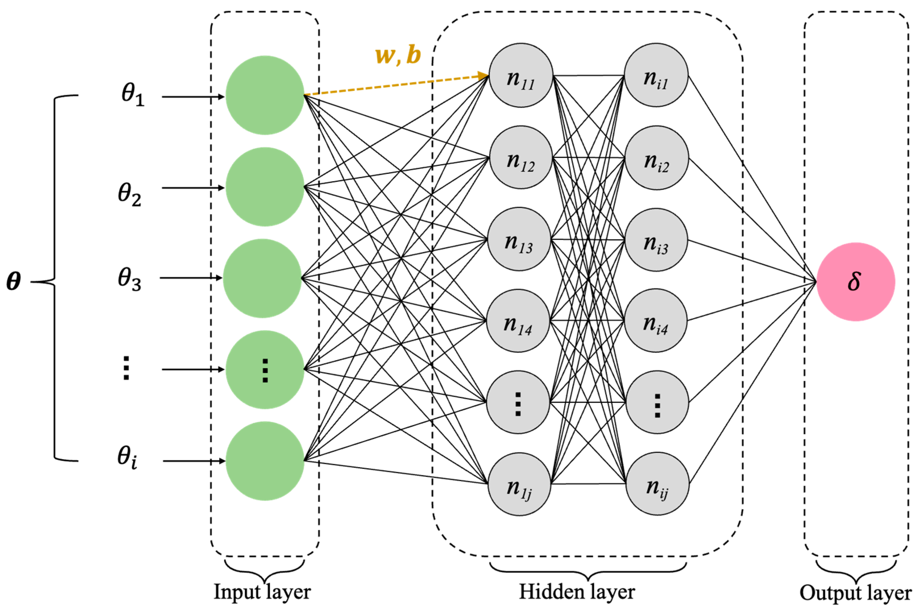
2.2.1. Static Neural Network: Multilayer Perceptron

In 1958, Rosenblatt introduced the perceptron and provided the perceptron convergence theorem [41]. A widely utilized supervised algorithm within feed-forward neural networks (FFNNs) is the multilayer perceptron (MLP). In MLP neural networks, the input parameter (θ) progresses unidimensionally from the input layer to the output layer (output results δ) via hidden layers [42], as illustrated in Figure 2.

A typical MLP comprises interconnected neurons n_ij, as shown in Figure 2, or processing elements. These neurons are organized into the following layers: an input layer; one or more hidden layers; and an output layer.

The performance of MLP in modeling non-linear relationships depends on the activation function used, such as ReLU, sigmoid, or Tanh. The ReLU activation function was employed in this work. ReLU is widely employed to detect the non-linear effect of various factors, defined as follows: f(x) is zero for x < 1, and f(x) equals x for x ≥ 0.

MLP neural networks are used to generalize a non-linear function $y_j^k$, where j and k of Equation (1) denote the generic neuron and hidden layer, respectively, in the tasks of function modeling with one predicted variable. The output is defined by [43]:

$$y_j^k=f(\sum _{i=1}^n{w}_{ij}^k{x}_i^k+b_i^k)$$

(1)

where $w_{ij}^k$ represents the weight of the connection between the ith neuron of the previous layer and the current neuron; $x_i^k$ is the input from the ith neuron of the preceding layer, and $b_i^k$ stands for the bias linked to the current neuron. The use of MLP allows for the approximation of non-linear mappings, which is useful in overcoming the issue of the non-linear relations among explanatory variables, particularly in the case of concrete dam seepage behavior [9].

2.2.2. Dynamic Neural Network

The Standard Recurrent Neural Networks

Recurrent neural networks (RNNs) represent a category of ANNs characterized by their dynamic behavior over time, owing to the interconnections between nodes forming either a directed or undirected graph across a time series [44]. These networks stem from feedback neural networks and possess the capability to handle input sequences of varying lengths by utilizing their internal state (memory), making them a kind of dynamic neural network. The basic architecture of the RNNs and the transfer processing are illustrated in Figure 3.

At each time step denoted as t, the activation $a^{<t>}$ and the output $y^{<t>}$ are defined as follows:

$$a^{<t>}=f_1\left(W_{aa}{a}^{<t-1>}+W_{ax}{x}^{<t>}+b_a\right)$$

(2)

$$y^{<t>}=f_2\left(W_{ya}{a}^{<t>}+b_y\right)$$

(3)

Here, $W_{ax}$, $W_{aa}$, $W_{ya}$, $b_a$, and $b_y$ are coefficients that are shared temporally, while $f_1$ and $f_2$ represent activation functions.

RNNs are commonly utilized to process sequential data. However, training RNNs can be challenging due to well-documented issues such as the vanishing and exploding gradient problems arising from the repeated multiplication of the recurrent weight matrix [45]. Additionally, they can struggle to learn long-term patterns [46]. Despite these drawbacks, RNNs possess feedback within their network architecture, which gives them the ability to represent and learn state processes. Due to the drawbacks of the RNNs, in this paper, advanced RNNs will be introduced to improve the prediction performance.

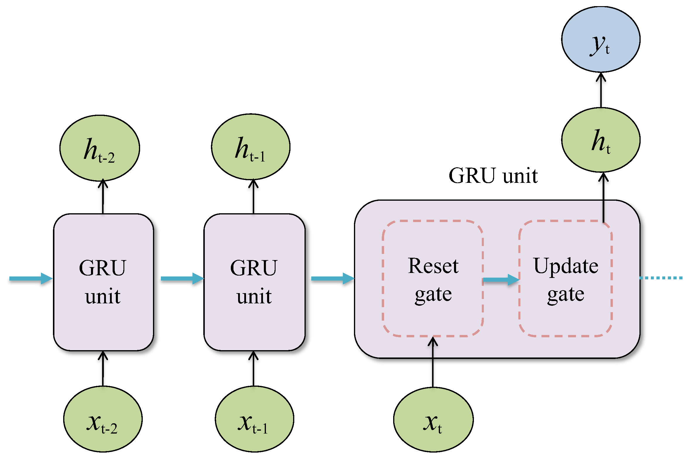
The Gated Recurrent Unit

The gated recurrent unit (GRU) represents an advanced type of RNN. Figure 4 displays the general structure of a GRU, depicting inputs for both the reset and update gates within the GRU architecture. The reset gate and update gate are used as vectors, each with entries in the range of (0, 1) to enable convex combinations. For example, the reset gate controls the extent to which the previous state is preserved, while the update gate governs how much of the new state replicates the old state. The learning rate, a parameter ranging from zero to one, determines the speed at which the weights are updated [47].

The input vector at time t is denoted as $x_t$. The output vectors of hidden units at time t are represented by $h_t$. These inputs are determined by the current time step’s input and the hidden state from the preceding time step. The outputs of these gates are produced through two fully connected layers with a sigmoid activation function, and $y_t$ depicts the outputs of the GRU.

The GRU [48] is a gate variant that is more streamlined and often offers comparable performance while being significantly faster to compute. Unlike MLP, in GRU, adjacent hidden neurons are connected. The sliding window allows for the sequential transfer of time-dependent input information through hidden units, enabling consideration of temporal correlations between events occurring at considerable temporal distances.

2.3. Optimization Methods

The ANNs require an optimizer to adjust the weights and biases based on the loss between the target and observed values. Stochastic gradient descent (SGD) is utilized to determine optimal weights to minimize prediction errors. This approach reduces the computational burden in high-dimensional optimization problems, resulting in faster iterations but at the cost of a lower convergence rate. Adam optimization serves as an extension of SGD and offers a more efficient alternative to traditional classical stochastic gradient descent for updating network weights. It adjusts the learning rate using squared gradients and incorporates momentum by utilizing a moving average of the gradient, similar to SGD with momentum. The Adam optimizer is a popular choice in machine learning. The Adam optimizer was selected in this study due to its applicability to various problem types, including those with sparse or noisy gradients. Its straightforward fine-tuning feature allows for quick and effective results.

3. Application Case: Montbel Dam, an Existing Earth Dam

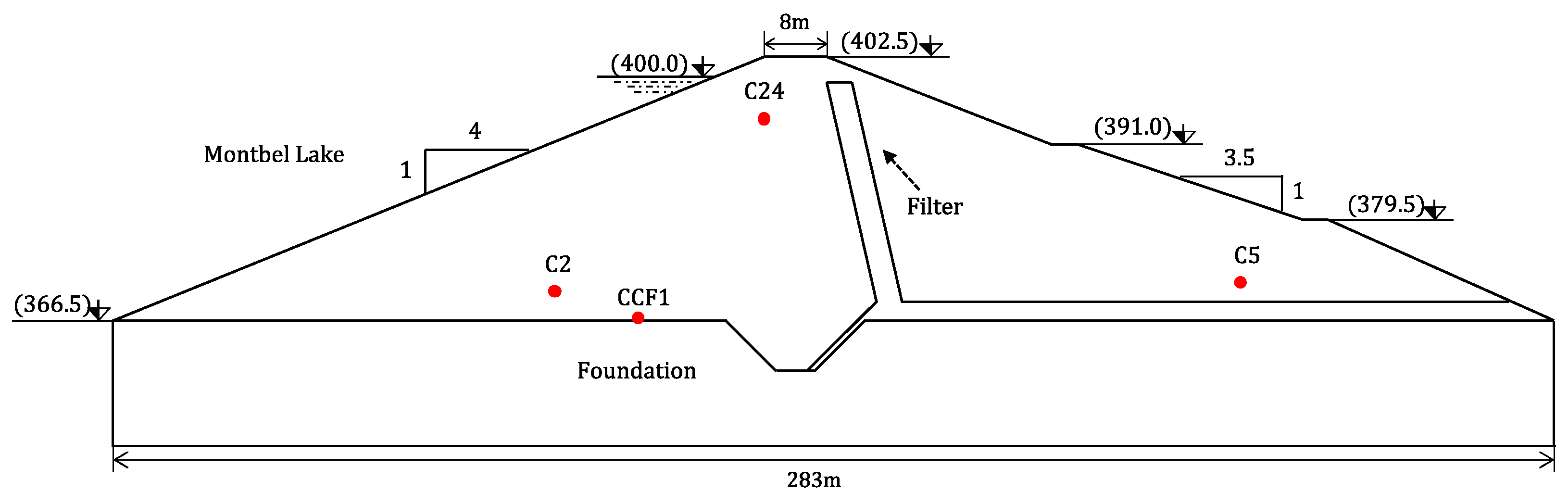
3.1. Description of the Case Study

This case study is a 36 m high earth dam used for irrigation, located in the region of Occitanie in France. Its reservoir has a volume of 60 million m³, and the normal water operating altitude level (400 m.a.s.l.) is 33.5 m above the altitude of the reservoir bottom (366.5 m.a.s.l.). The dam studied is a homogeneous embankment dam made of marl with very low permeability. The dam was built between 1982 and 1985. The body of the dam is equipped with a semi-vertical drain extended horizontally by a drainage mat.

Piezometers are used to measure pore water pressure in the soil mass of the dam. They provide significant quantitative data on the magnitude and distribution of pore water pressure with time. Forty-five automatic piezometers (PWP cells) were distributed at different positions of the dam. They were used to measure PWP inside the dam and the foundation.

Although the selected monitoring section has 10 sensors, some monitoring data are in poor regularity, with interrupted monitoring or recording errors. Therefore, the most representative four monitoring points (with the completed dataset, marked with red points in Figure 5, including C2 (upstream of the dam body), C5 (downstream of the dam body), CCF1 (foundation of the dam), and C24 (near the filter) are selected for the building prediction model.

3.2. Dataset Preparation

The PWPs have been monitored every month (or twice a month) from 1990 to 2019, and 450 data sets were available. Different factors are influential for the PWP, such as the hydrostatic level (H), season (S), and time or irreversible effects (T) [4]. Lagged features are the classic way to transform a time series prediction problem into a supervised learning problem. The simplest approach is to predict the f (t + 1) value given the previous value f (t − 1), which can represent the time effect. The hydrostatic (H) factor is defined by the hydraulic head, which measures the reservoir level. The seasonal (S) effect is intended to represent the day of the year (e.g., 1 to 365) corresponding to the measurement. One typical expression of this factor is given in Equation (4) below, in which the season $S_i$ is an angle equaling to 0 on the 1st of January and $2\pi$ on the 31st of December [4].

$$S_i=\frac{2\pi (t_i-t_0)}{365}$$

(4)

where $t_i$ and $t_0$ are, respectively, the day of the currently analyzed measurement and the initial reference date for the data, with $t_i$ also standing for the factor of irreversible effects T. The dataset is shown in

Table 1. Summary of range for input and target output variables (C2).

Parameter	Min	Max	Mean	Unit
Hydrostatic (H)	382.42	400.27	394.8	m
Season (S)	0	6.27	3.118	radian
Time (T)	0	10,939	6327	day
Pore water pressure (PWP)	77.3	131.6	100.8	kPa

, and it has been divided randomly into training datasets (352), validation datasets (44), and test datasets (44). The ML model function is defined by

$$f\left(t+1\right)=f\left(H\left(t\right),S\left(t\right),T, f(t-1)\right)$$

(5)

Pearson coefficients demonstrate that the four factors, T, H, f (t − 1), have a relatively large effect on the PWP, as shown in Figure 6. Although S has a limited influence on PWP, in this case, its effect should be considered for building a more general prediction model in theory [47]. The first histogram, “T”, shows that the frequency of measurements has doubled in the last several years, which has an impact (correlation coefficient is −0.743) on the variable P(t − 1) corresponding to the previous measurement. For most measurements, P(t − 1) corresponds to the measurement made 1 month before, but for the measurements of the last several years, P(t − 1) corresponds to the measurement made 2 weeks before. The value and distribution are shown by yellow histograms, and cloud graphs represent areas of concentration, trends, and changes in the data (in terms of two kinds of data), making it easier to discover the structure and patterns of the dataset. For example, in the cloud graph of T and S (noted as “a1b”), T concentrates more in the latest years, and S has two peaks, which are approximately symmetrically distributed with a mean value of 3.118.

Before inputting the dataset, some preprocessing work should be conducted so that convergence velocity as well as accuracy can be improved drastically. The MinMaxScaler is a normalization method, which scales each feature to a designated range of [0, 1], utilizing two parameters: the lower and the upper bounds [49]. Normalization is a basic procedure before training the model by any ML method, providing a good ability to decrease the probability of overfitting and enhance the generalization. The MinMaxScaler is defined by

$$x_{\left(\mathrm{0,1}\right)}=\frac{x_i-X_{Min}}{X_{Max}-X_{Min}}$$

(6)

where $x_i$ represents the original data, and $x_{\left(\mathrm{0,1}\right)}$ is the normalized data; $X_{Min}$ and $X_{Max}$ denote the minimum and maximum values of the complete dataset, encompassing data for training, validating, and testing. After training and obtaining the optimized ML model, the predicted results could apply the inverse normalization method to obtain the observed PWP value.

3.3. Development of Machine Learning Models

All the ML models utilized in this investigation were developed using the Keras package of Python, a high-level application programming interface designed for neural networks. The computations were executed on an Intel(R) Xeon(R) CPU E5-2609 v4 @ 1.70 GHz with 32 G RAM (Intel, Santa Clara, CA, USA). Optimal hyperparameters were obtained based on the prediction performance, assessed using the coefficient of determination (R²) and the mean square error (MSE):

$$R^2=1-\frac{{\sum }_{i=1}^n(m_i-p_i{)}^2}{{\sum }_{i=1}^n(m_i-\overline{m}{)}^2}$$

(7)

$$MSE=\frac{1}{n}\sum _{i=1}^n(m_i-p_i{)}^2$$

(8)

where $m_i$ and $p_i$ represent the measurement and prediction of the PWP, respectively; $\overline{m}$ is the mean of the measurement. The loss function is also defined by MSE. It is important to note that the models exhibiting superior performance are those with higher R² values and lower MSE values.

4. Results and Discussion

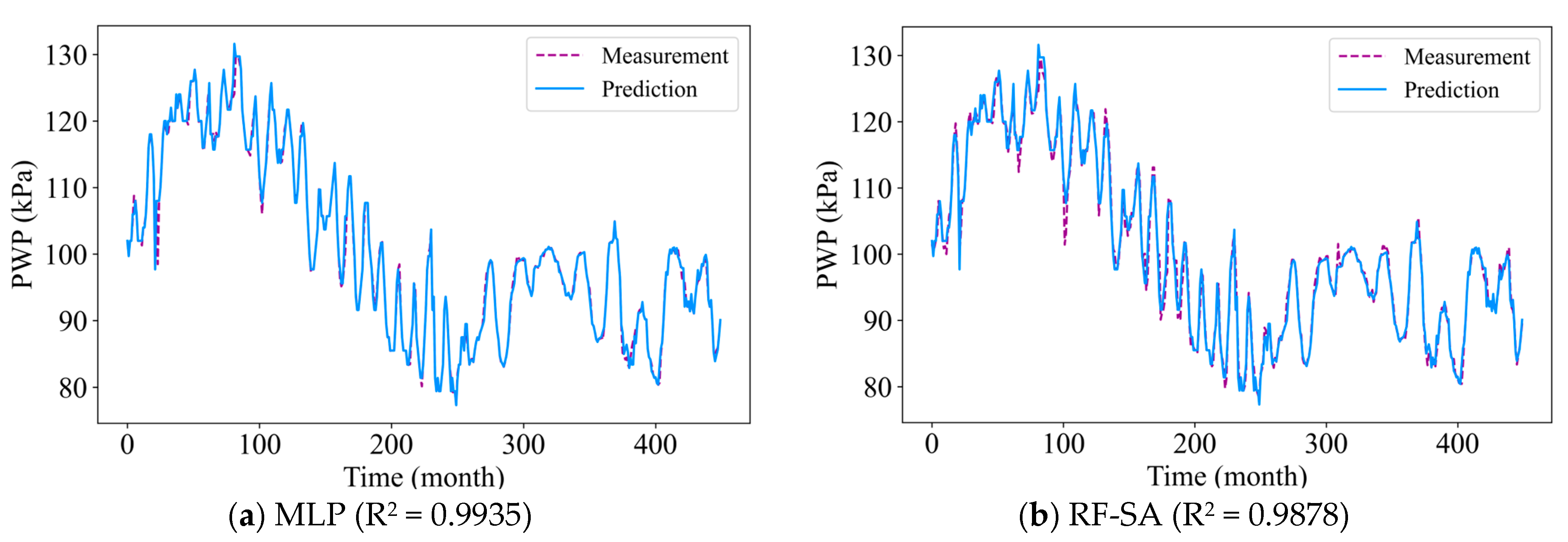
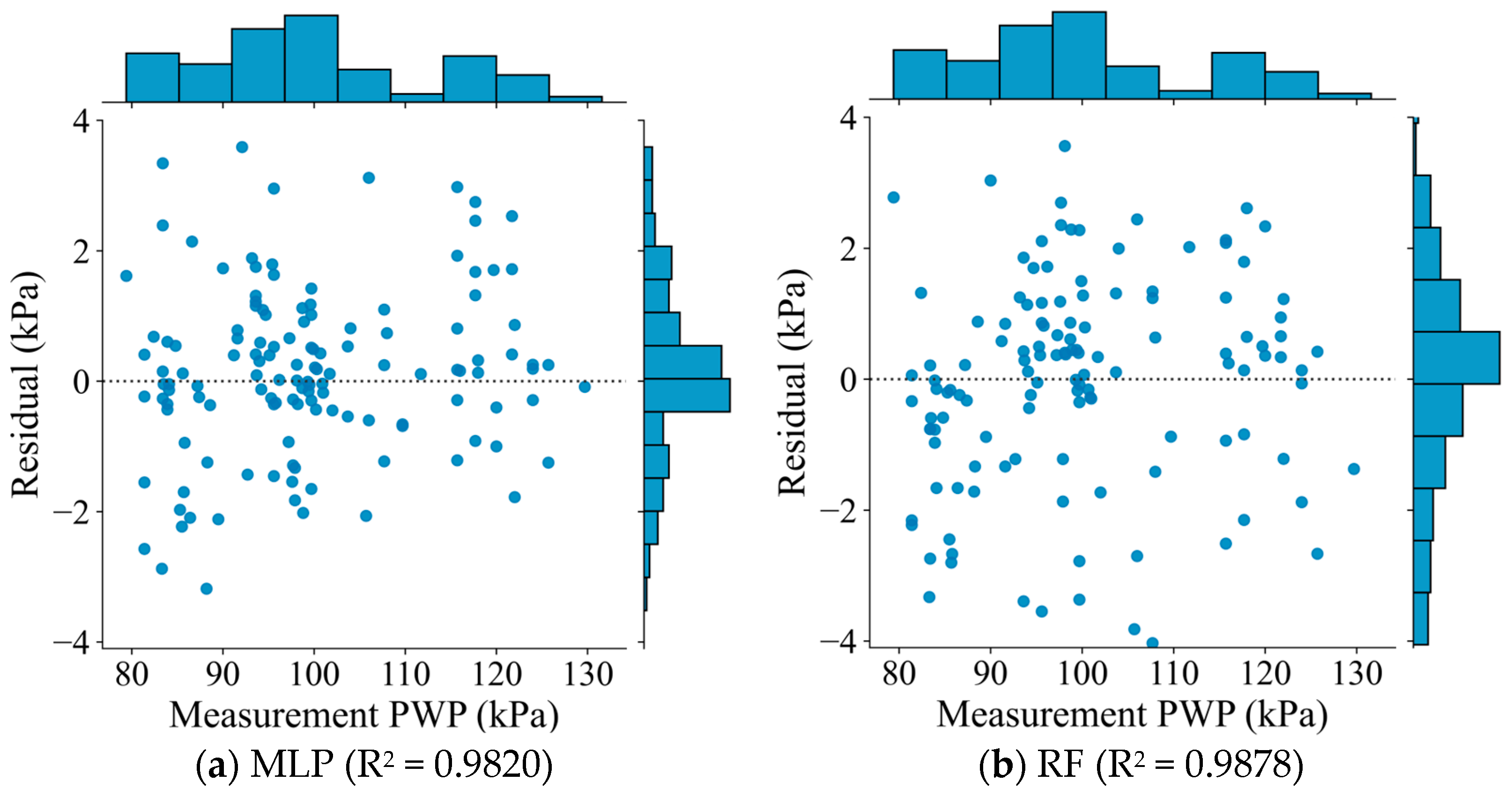
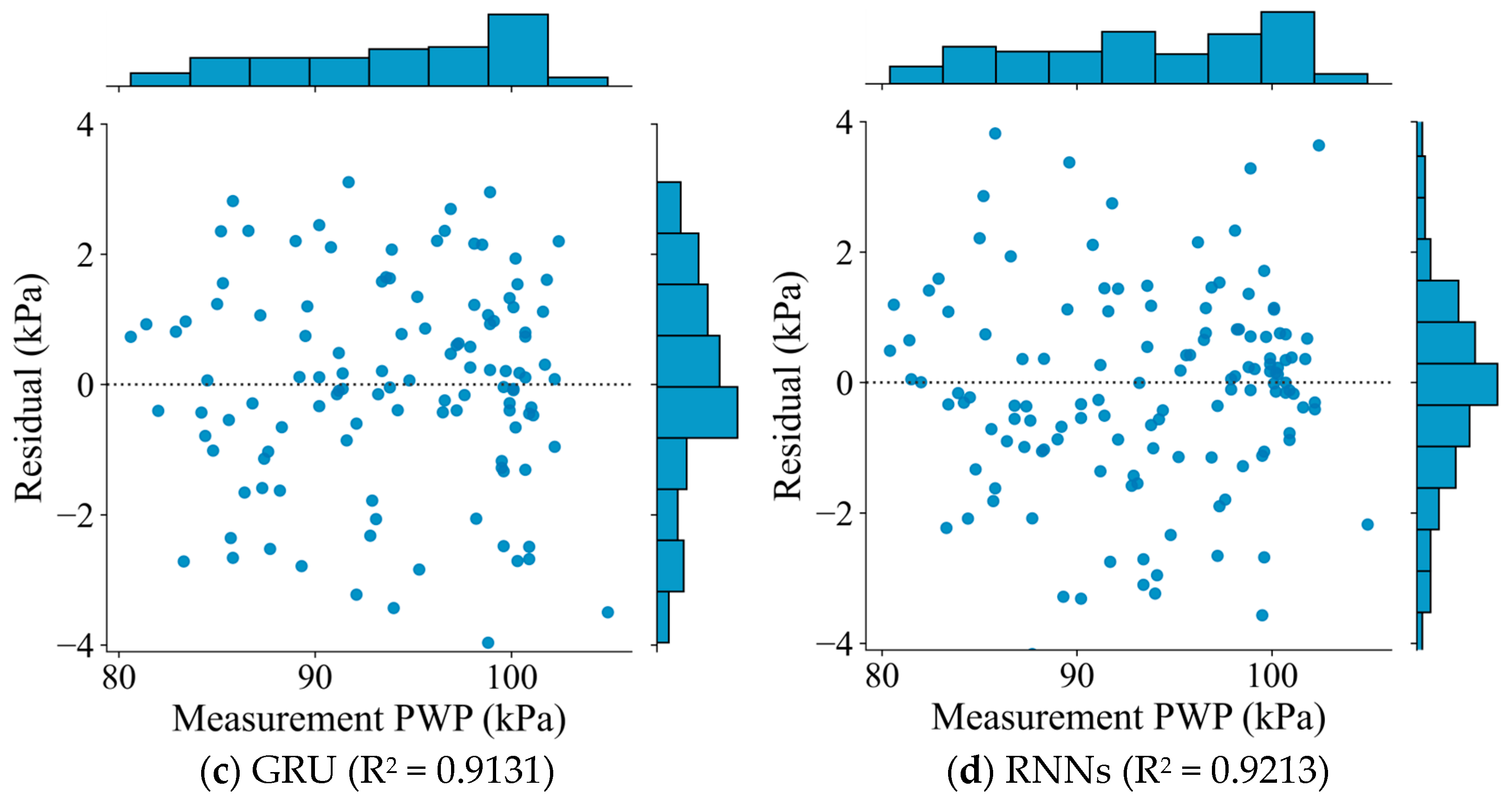
4.1. Model Performance and Comparison

The results of ML models for C2 are presented in Figure 7. They show the powerful prediction capability of the four methods. This may be due to a number of factors. Firstly, the model input variables (hydrostatic, season, time, etc.) explain a large portion of the variations in PWP, for example, higher PWP for a full reservoir (and lower for a low reservoir level), higher PWP in winter and lower PWP in summer. In addition, several values of the hyper-parameters were tested before arriving at a satisfactory model.

These ML models can be useful in detecting pathology or abnormal behavior of the dam, such as an increase in PWP, that is not explained by a reversible variation in the level of the reservoir or by the season.

It should be remembered that the case study relates to the prediction of time series. The dataset has been divided randomly into training data sets (352), validation datasets (44), and test datasets (44).

Table 2. Optimized hyperparameters applied in RF-SA model of C2 piezometer after optimization.

Hyperparameters	Meanings	Value
n_estimators	The number of trees in the forest.	14
max_depth	The maximum depth of the tree.	18
min_samples_leaf	The minimum number of samples required to be at a leaf node.	1
random_state	The number of random seeds to ensure the same results when inputting the same number.	11

shows the optimized hyperparameters applied in the RF-SA model.

Table 3. Prediction performance and efficiency of ML models (both training and testing datasets).

Method		MSE (kPa2)	R2	CPU Training Time (s)
MLP	Mean	0.0087	0.9949	8.14
	Max	0.0091	0.9935	10.35
	Min	0.0066	0.9912	7.12
RF	Mean	0.021	0.9801	52.13
	Max	0.0259	0.9878	96.56
	Min	0.0194	0.9766	12.34
RNNs	Mean	0.0657	0.9601	7.22
	Max	0.0799	0.9623	10.26
	Min	0.0511	0.9594	5.54
GRU	Mean	0.0623	0.9689	27.16
	Max	0.0746	0.9717	37.22
	Min	0.0435	0.9702	19.42

presents the prediction performance and efficiency of the ML models on the training and test datasets.

Table 4. The accuracy comparison of prediction model for four piezometers (testing datasets).

Model	Sensor	MSE (kPa2)	R2
1	C2	0.0292	0.9820
2	C5	0.0051	0.9981
3	C24	0.0040 *	0.9034
4	CCF1	0.0073	0.9925

* MSE is relatively low because PWP of C24 has a small variation compared to C2, C5, and CCF1.

shows the performance of the prediction models on the test datasets.

For the static PWP prediction, there are two types of models: one is established by the MLP method; the other is obtained by random forest combined with simulated annealing (RF-SA). Hyperparameters are set before the learning process begins. For the MLP model, the optimized hyperparameters (learning rate = 0.01, decay = 1 × 10⁻⁶, and momentum = 0.9) used a test size equal to 30% of the dataset. Both the testing and training R² values reached 0.98 (as seen in Figure 7a), signifying the robust prediction capability of the MLP model.

For the RF-SA model, the R² reaches 0.98, as shown in Figure 7b, which is similar to the performance of the MLP model. The single RF training time is so rapid that it only takes several seconds, and commonly, single training results do not seem to be very accurate (R² = 0.92). After optimizing the hyperparameters, the model performance improved. All of the implications and optimal values of the hyperparameters by applying SA in the RF models are shown in Table 2. The optimized model is a distribution of 14 decision trees, and every tree would re-split less than 18 times. The SA processing increases the accuracy (R² increases from 0.92 to 0.98), while on average, the efficiency of RF-SA is a little lower than MLP by contrast to the CPU training time shown in Table 3.

The PWP prediction models are also built by the classic RNNs and GRU methods. The training results show that the accuracy of RNNs and GRU models could achieve 0.96 and 0.97, respectively. Comparing all ML models, the MLP model can predict PWP most accurately. The reason why deep learning methods perform inadequately is that the database consists of 440 groups, which is not enough for training a deep learning model. It is evident that the larger the number of databases, the more accurate the deep learning model, which has powerful robustness for both interpolation and exploitation. The convergence efficiency of MLP is much better than that of RF-SA in terms of similar accuracy, which indicates that the architecture of MLP is more suitable for the small time series database, and the corresponding optimization method is more economical and robust. Some of the studies indicate that RF is good at classification issues based on high-dimensional, small-size databases [50].

Therefore, the PWP prediction models of the other three sensors (C5, C24, CCF1) are built with MLP, as shown in Table 4. Measurements from earlier decades are still influenced by the PWP dissipation processes caused by dam construction, and this aspect is well-represented in the four prediction models.

The dynamic neural networks can memorize the characters inputted by time step, and especially GRU can remember the effects more intelligently by gate units. Several gates allow us to select the most important properties and sensitively evaluate the weight sensitivity. Then, the accuracy of the model could achieve 0.97, and the MSE is less than 0.007 kPa. The ability to predict depends not only on the hyperparameters but also on the architecture. These analytical procedures and the results obtained from them are described in the next section. A higher number of epochs refers to the model completing more iterations of both forward and backward passes across all training batch sizes. This allows the model to capture more information and adjust weights from the dataset. The most proper hyperparameters (with underline) in the GRU model are shown in

Table 5. Optimized hyperparameters applied in GRU of C2 piezometer after optimization.

Hyperparameters	Meanings	Value
n_neurons	The number of neurons in hidden layer.	50, 100, 150, 200, 250, 300
n_layers	The number of layers in network (hidden layer and output layer).	2, 3, 4, 5, 6, 7
n_epochs	The times of the one forward pass and one backward pass of all the training examples.	10, 20, 30, 40, 50, 60, 70, 80, 90
learning_rate	The learning rate is a hyperparameter that controls how much to change the model in response to the estimated error each time the model weight is updated.	0.01, 0.001, 0.0001
batch_size	The number of training examples utilized in one iteration.	2, 4, 8, 16, 32, 64

The underlined values correspond to the optimal values among the tested values.

, which are obtained from the loop algorithm.

Because of the random training mechanism, the model is different every time. Therefore, the hyperparameters should be validated at least 10 times. The maximum, minimum, and statistic mean of R², MSE, and CPU running times of different models are shown in Table 3, which demonstrates the accuracy and efficiency of the prediction capability.

The testing results are shown in Figure 8. The accuracy of the RF and MLP models is similar; however, the MLP is slightly more efficient than the RF-SA. From the histogram, the residual density distribution is normal, with a mean equal to zero. They both have a powerful ability to predict the PWP, which is validated by the testing simulation performance. In the feedback neural networks, the GRU model is more robust than the standard RNNs. That is because GRU is better for long-term memory than the standard RNNs. Hydraulic behavior is not only decided by recent hydrostatic events but also by the structure’s evolution over several decades. For example, in the case study, early decade measurements are still affected by the PWP dissipation process from the dam construction, and this aspect is well-reproduced by the different models used in this paper.

Static ML models perform better for interpolation rather than extrapolation. Therefore, the accuracy of the static ML training model is reliable for the ranges of values of H, S, and $T$, f (t − 1), previously given in Table 1. When the training set is large enough, dynamic neural networks perform better on inputting extrapolative datasets. In the other case [3], the RNNs and GRU have a higher accuracy than static ANNs in predicting PWP. However, due to the frequency of PWP measurement in this study case, which is not enough for dynamic neural networks to study the features accurately, the accuracy seems worse than for the static ML models.

From the comparison results, it is summarized that when the database is small and low-dimensional in size, employing classical MLP is more efficient and accurate. When the database is small and has high dimensions, the RF seems more capable. When the database is large enough, with thousands or more datasets, deep learning techniques perform better and can learn more non-linear relationships from the inputs and target outputs. Consequently, for different case studies, the different ML methods should be attempted to make a comparison.

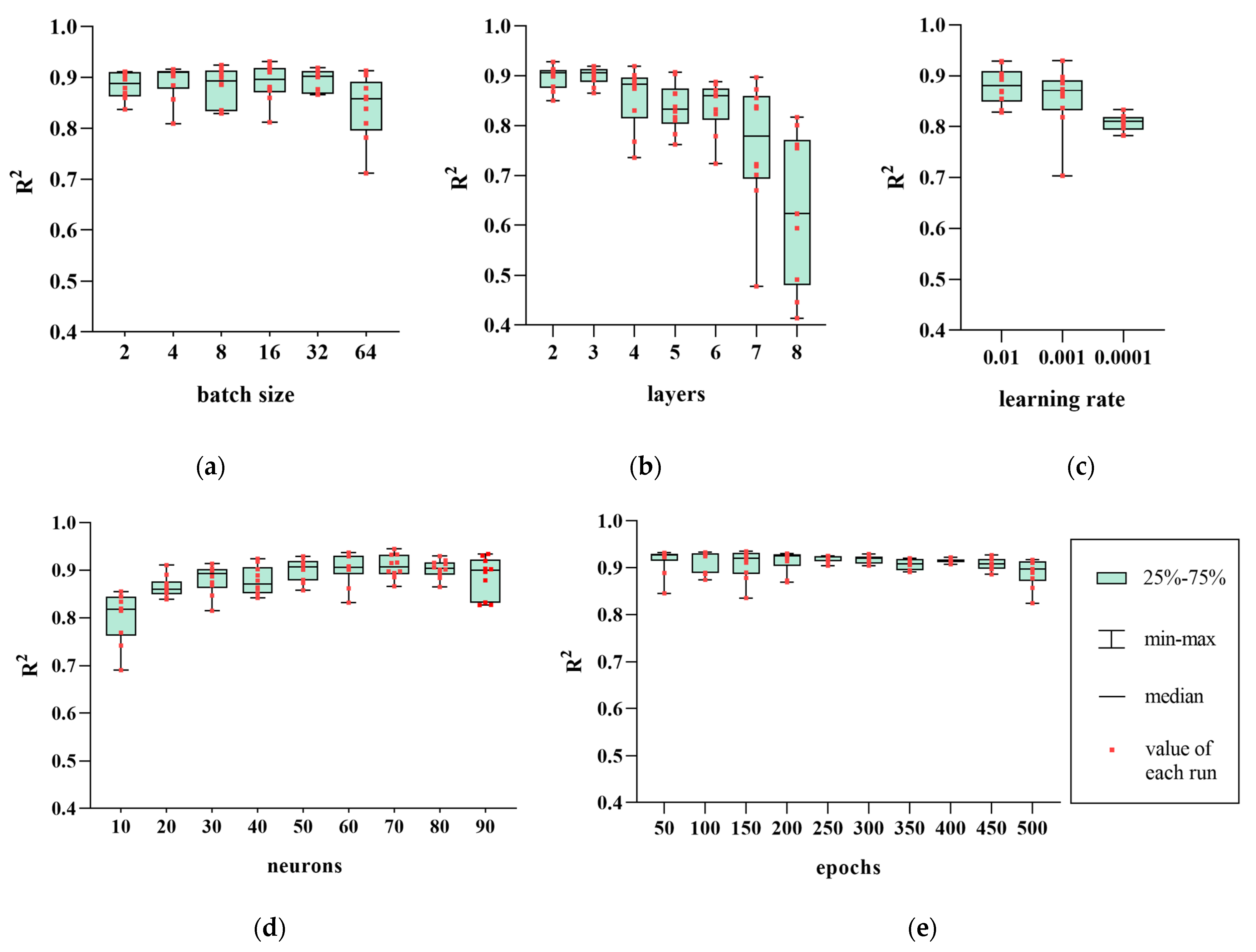
4.2. Sensitivity Analysis

The speed of convergence and expressive power of ML predictive models are affected not only by the architecture of the model but also by the choice of hyperparameters. In the case of the neural network series of ML, the architectural parameters are the number of hidden layers and the number of neurons in the hidden layers. The hyperparameters are learning rate, number of epochs, and number of samples (batch size) per learning.

In this part, the GRU method is used to investigate the impacts of the hyperparameters in neural network architecture. These parameters are tunable and can directly affect how well a model performs. The values of hyperparameters are listed in Table 5; among them is the value, which is bolder and underlined, selected as the fixed value when one of the parameters changes, as shown in the variables. Every set of hyperparameters is validated 10 times.

The batch size determines the number of samples that pass through the network during training. In an entire epoch, the overall N samples are divided into N/batch_size datasets. The learning is taken from the first dataset to the last one. Smaller batch sizes require less memory since the network is trained on fewer samples, reducing the overall memory demand during training. This is important, especially if the whole dataset is so enormous that it cannot be trained using an ordinary computer. Since the memory of the computer is always set as a power series of 2, the batch size is also defined as the same as the memory value. Figure 9a illustrates that the accuracy on testing datasets increases with smaller batch sizes, up until a batch size of 16, beyond which it sharply declines. Typically, networks are trained faster with mini-batches. This is because the networks update the weight after each propagation. Therefore, the batch size set of 16 is more efficient in modeling the PWP of this case study.

The layers and neurons are seen as the basic model properties, which are determined by the model complexity. No hidden layers are needed if the data are regularly linearly distributed. For less complex data with fewer features, neural networks with one to two hidden layers are sufficient, as shown in Figure 9b. If data have large features, it will be necessary to use three to five hidden layers to obtain an optimum solution [13]. One or two hidden layers can be enough because the raw data have few features and reveal some kind of non-linear behavior. The larger the neurons, the more complicated the model. What stands out in Figure 9d is that 70 neurons are enough for the prediction of C2 PWP (when the number of neurons increases from 70 to 80, R² becomes smaller).

The learning rate stands out as a crucial hyperparameter in configuring neural networks. Choosing a proper learning rate is a delicate balance, as too small a value could lead to a lengthy training process with potential stagnation, while a value that is too large might result in rapid learning of sub-optimal weights or an unstable training process. Therefore, it is essential to examine the impact of the learning rate on model performance and gain practical insights into how it influences the model’s behavior. In this GRU model, the number of R² is likely to continue decreasing with the fall of the learning rate, as shown in Figure 9c. What can be clearly seen in this figure is that the R² rises to a high point and peaks when the learning rate equals 0.001.

As seen in Figure 10, the loss (MSE) decreases with epoch times increase. However, more epochs do not mean that the model is more accurate, as shown in Figure 9e. The overfitting phenomenon may happen when the epochs are exaggerated in neural networks. Such a phenomenon could occur in the MLP model as well. When it happens, the training epoch needs to be decreased so as to learn less noise and detail of the dataset evolution. It can be noticed that the impact of varying batch sizes and epochs on model performance is not as pronounced as the effects of varying the number of hidden layers, learning rate, and neurons.

The training results of ANNs could be improved greatly by optimizing the hyperparameters, especially the value of hidden layers and neurons. In the case of this study, the optimization of learning rate, batch size, and epochs did not significantly improve the accuracy of the model. These sensitivity analyses of hyperparameters offer a reference tutorial for the ANNs tuning.

5. Conclusions

In this paper, four different ML methods have been applied to build the PWP prediction models. It has been highlighted that both the static and dynamic neuron networks have a good ability (R² = 0.99) to predict the monitoring PWP in an earth dam. The findings of this study suggest that among four different ML methods, the MLP and RF-SA are more intelligent and accurate for predicting the PWP response. GRUs have a better prediction performance than RNNs in dynamic neural networks. Because the monitoring frequency of PWP in this study case is not enough for dynamic neural networks to study the features accurately, the accuracy of RNNs (which is appropriate for time-series prediction) is worse than that of the static ML models. Therefore, for different case studies, an attempt should be conducted to compare different ML approaches in order to select the best prediction method. In summary, the machine learning methods have some significant advantages in predicting the PWP of hydraulic response. In this case study, early decade measurements are still affected by the PWP dissipation process from the dam construction, and this aspect is well-reproduced by the different models used in this paper. These models can also demonstrate the soil’s non-linear properties. The models established by ML methods are very flexible and do not need additional physical assumptions. They can be used in different earth dam positions, even in different dams.

The architecture of the RF model could be optimized by the SA method efficiently, and the R² could be improved from 0.92 to 0.98. The architectures of ANN models, including MLP, RNNs, and GRU, could be optimized by the Adam method and loop algorithm. The optimizing processes reveal that different batch sizes and epochs do not affect model performance as significantly as different numbers of hidden layers, learning rates, and neurons. The sensitivity analysis of these hyperparameters provides a reference for the tuning of ANNs for other machine learning applicators. By optimizing the hyperparameters (especially the value of hidden layers and neurons), the training results of ANNs can be greatly improved.

The weaknesses of ML methods should also be noted. These methods rely on a large number of training datasets in which the input and output should be highly correlated. Most of the study cases do not have enough datasets, and there is a large uncertainty in the influence of the actual measured data. Therefore, an adequate amount of data is the basis for successful modeling in this study case.

References

1. Abdel-Ghaffar, A.M.; Scott, R.F. Analysis of Earth Dam Response to Earthquakes. J. Geotech. Eng. 1979, 105, 1379–1404. [Google Scholar] [CrossRef]
2. Fattah, M.; Omran, H.; Hassan, M. Behavior of an Earth Dam during Rapid Drawdown of Water in Reservoir—Case Study. Int. J. Adv. Res. 2015, 3, 110–122. [Google Scholar]
3. Wei, X.; Zhang, L.; Yang, H.-Q.; Zhang, L.; Yao, Y.-P. Machine learning for pore-water pressure time-series prediction: Application of recurrent neural networks. Geosci. Front. 2021, 12, 453–467. [Google Scholar] [CrossRef]
4. Guo, X.; Baroth, J.; Dias, D.; Simon, A. An analytical model for the monitoring of pore water pressure inside embankment dams. Eng. Struct. 2018, 160, 356–365. [Google Scholar] [CrossRef]
5. Ng, C.W.W.; Liu, H.W.; Feng, S. Analytical solutions for calculating pore-water pressure in an infinite unsaturated slope with different root architectures. Can. Geotech. J. 2015, 52, 1981–1992. [Google Scholar] [CrossRef]
6. Mouyeaux, A.; Carvajal, C.; Bressolette, P.; Peyras, L.; Breul, P.; Bacconnet, C. Probabilistic analysis of pore water pressures of an earth dam using a random finite element approach based on field data. Eng. Geol. 2019, 259, 105190. [Google Scholar] [CrossRef]
7. Venkatesh, K.; Karumanchi, S.R. Distribution of pore water pressure in an earthen dam considering unsaturated-saturated seepage analysis. E3S Web Conf. 2016, 9, 19004. [Google Scholar] [CrossRef]
8. Tufano, R.; Formetta, G.; Calcaterra, D.; De Vita, P. Hydrological control of soil thickness spatial variability on the initiation of rainfall-induced shallow landslides using a three-dimensional model. Landslides 2021, 18, 3367–3380. [Google Scholar] [CrossRef]
9. de Granrut, M.; Simon, A.; Dias, D. Artificial neural networks for the interpretation of piezometric levels at the rock-concrete interface of arch dams. Eng. Struct. 2019, 178, 616–634. [Google Scholar] [CrossRef]
10. Anello, M.; Bittelli, M.; Bordoni, M.; Laurini, F.; Meisina, C.; Riani, M.; Valentino, R. Robust Statistical Processing of Long-Time Data Series to Estimate Soil Water Content. Math. Geosci. 2024, 56, 3–26. [Google Scholar] [CrossRef]
11. Cho, S.E. Probabilistic analysis of seepage that considers the spatial variability of permeability for an embankment on soil foundation. Eng. Geol. 2012, 133–134, 30–39. [Google Scholar] [CrossRef]
12. Fenton, G.A.; Griffiths, D.V. Statistics of Free Surface Flow through Stochastic Earth Dam. J. Geotech. Eng. 1996, 122, 427–436. [Google Scholar] [CrossRef]
13. Salazar, F.; Morán, R.; Toledo, M.Á.; Oñate, E. Data-Based Models for the Prediction of Dam Behaviour: A Review and Some Methodological Considerations. Arch. Computat. Methods Eng. 2017, 24, 1–21. [Google Scholar] [CrossRef]
14. Li, B.; Yang, J.; Hu, D. Dam monitoring data analysis methods: A literature review. Struct. Control Health Monit. 2020, 27, e2501. [Google Scholar] [CrossRef]
15. Makasis, N.; Narsilio, G.A.; Bidarmaghz, A. A machine learning approach to energy pile design. Comput. Geotech. 2018, 97, 189–203. [Google Scholar] [CrossRef]
16. Habibagahi, G.; Bamdad, A. A neural network framework for mechanical behavior of unsaturated soils. Can. Geotech. J. 2003, 40, 684–693. [Google Scholar] [CrossRef]
17. Goh, A.T.C.; Zhang, R.H.; Wang, W.; Wang, L.; Liu, H.L.; Zhang, W.G. Numerical study of the effects of groundwater drawdown on ground settlement for excavation in residual soils. Acta Geotech. 2020, 15, 1259–1272. [Google Scholar] [CrossRef]
18. Huang, F.-K.; Wang, G.S. ANN-based Reliability Analysis for Deep Excavation. In Proceedings of the EUROCON 2007-The International Conference on “Computer as a Tool”, Warsaw, Poland, 9–12 September 2007; pp. 2039–2046. [Google Scholar] [CrossRef]
19. Lu, Q.; Chan, C.L.; Low, B. Probabilistic evaluation of ground-support interaction for deep rock excavation using artificial neural network and uniform design. Tunn. Undergr. Space Technol. 2012, 32, 1–18. [Google Scholar] [CrossRef]
20. Demirkaya, S.; Balcilar, M. The Contribution of Soft Computing Techniques for the Interpretation of Dam Deformation. In Proceedings of the FIG Working Week, Roma, Italy, 6–12 May 2012. [Google Scholar]
21. Su, H.; Chen, Z.; Wen, Z. Performance improvement method of support vector machine-based model monitoring dam safety: Performance Improvement Method of Monitoring Model of Dam Safety. Struct. Control Health Monit. 2016, 23, 252–266. [Google Scholar] [CrossRef]
22. Bouayad, D.; Emeriault, F. Modeling the relationship between ground surface settlements induced by shield tunneling and the operational and geological parameters based on the hybrid PCA/ANFIS method. Tunn. Undergr. Space Technol. 2017, 68, 142–152. [Google Scholar] [CrossRef]
23. Puri, N.; Prasad, H.D.; Jain, A. Prediction of Geotechnical Parameters Using Machine Learning Techniques. Procedia Comput. Sci. 2018, 125, 509–517. [Google Scholar] [CrossRef]
24. Belmokre, A.; Mihoubi, M.; Santillan, D. Analysis of dam beaviour by statistical models: Application of the random forest approach. KSCE J. Civ. Eng. 2011, 23, 4800–4811. [Google Scholar] [CrossRef]
25. Mata, J. Interpretation of concrete dam behaviour with artificial neural network and multiple linear regression models. Eng. Struct. 2011, 33, 903–910. [Google Scholar] [CrossRef]
26. Mata, J.; Tavares de Castro, A.; Sa da Costa, J. Constructing statistical models for arch dam deformation. Struct. Control. Health Monit. 2014, 21, 423–437. [Google Scholar] [CrossRef]
27. Dai, B.; Gu, C.; Zhao, E.; Qin, X. Statistical model optimized random forest regression model for concrete dam deformation monitoring. Struct. Control Health Monit. 2018, 25, e2170. [Google Scholar] [CrossRef]
28. Hellgren, R.; Malm, R.; Ansell, A. Performance of data-based models for early detection of damage in concrete dams. Struct. Infrastruct. Eng. 2021, 17, 275–289. [Google Scholar] [CrossRef]
29. Tinoco, J.; de Granrut, M.; Dias, D.; Miranda, T.; Simon, A.G. Piezometric level prediction based on data mining techniques. Neural Comput. Appl. 2020, 32, 4009–4024. [Google Scholar] [CrossRef]
30. Kim, Y.S.; Kim, B.T. Prediction of relative crest settlement of concrete-faced rockfill dams analyzed using an artificial neural network model. Comput. Geotech. 2008, 35, 313–322. [Google Scholar] [CrossRef]
31. Mustafa, M.R.; Rezaur, R.B.; Saiedi, S.; Rahardjo, H.; Isa, M.H. Evaluation of MLP-ANN Training Algorithms for Modeling Soil Pore-Water Pressure Responses to Rainfall. J. Hydrol. Eng. 2013, 18, 50–57. [Google Scholar] [CrossRef]
32. Mohammed, M.; Watanabe, K.; Takeuchi, S. Grey model for prediction of pore pressure change. Environ. Earth Sci. 2010, 60, 1523–1534. [Google Scholar] [CrossRef]
33. Tayfur, G.; Swiatek, D.; Wita, A.; Singh, V.P. Case Study: Finite Element Method and Artificial Neural Network Models for Flow through Jeziorsko Earthfill Dam in Poland. J. Hydraul. Eng. 2005, 131, 431–440. [Google Scholar] [CrossRef]
34. Beiranvand, B.; Rajaee, T. Application of artificial intelligence-based single and hybrid models in predicting seepage and pore water pressure of dams: A state-of-the-art review. Adv. Eng. Softw. 2022, 173, 103268. [Google Scholar] [CrossRef]
35. El Bilali, A.; Moukhliss, M.; Taleb, A.; Nafii, A.; Alabjah, B.; Brouziyne, Y.; Mazigh, N.; Teznine, K.; Mhamed, M. Predicting daily pore water pressure in embankment dam: Empowering Machine Learning-based modeling. Environ. Sci. Pollut. Res. 2022, 29, 47382–47398. [Google Scholar] [CrossRef]
36. Qin, S.; Xu, T.; Zhou, W.-H. Predicting Pore-Water Pressure in Front of a TBM Using a Deep Learning Approach. Int. J. Geomech. 2021, 21, 04021140. [Google Scholar] [CrossRef]
37. Breiman, L. Random Forests. Mach. Learn. 2001, 45, 5–32. [Google Scholar] [CrossRef]
38. Kirkpatrick, S.; Gelatt, C.D.; Vecchi, M.P. Optimization by Simulated Annealing. Science 1983, 220, 671–680. [Google Scholar] [CrossRef] [PubMed]
39. Bhanot, G. The Metropolis algorithm. Rep. Prog. Phys. 1988, 51, 429–457. [Google Scholar] [CrossRef]
40. Freiman, M.H. Using Random Forests and Simulated Annealing to Predict Probabilities of Election to the Baseball Hall of Fame. J. Quant. Anal. Sports 2010, 6, 1–35. [Google Scholar] [CrossRef]
41. Rosenblatt, F. The perceptron: A probabilistic model for information storage and organization in the brain. Psychol. Rev. 1958, 65, 386–408. [Google Scholar] [CrossRef]
42. Millar, D.L.; Clarici, E.; Calderbank, P.A.; Marsden, J.R. On the practical use of a neural network strategy for the modelling of the deformability behaviour of Croslands Hill sandstone rock. In International Journal of Rock Mechanics and Mining Sciences and Geomechanics Abstracts; Elsevier: Amsterdam, The Netherlands, 1995; Volume 495, pp. 457–465. [Google Scholar]
43. Bre, F.; Gimenez, J.M.; Fachinotti, V.D. Prediction of wind pressure coefficients on building surfaces using artificial neural networks. Energy Build. 2018, 158, 1429–1441. [Google Scholar] [CrossRef]
44. Elman, J.L. Finding structure in time. Cogn. Sci. 1990, 14, 179–211. [Google Scholar] [CrossRef]
45. Omlin, C.W.; Giles, C.L. Constructing deterministic finite-state automata in recurrent neural networks. J. ACM 1996, 43, 937–972. [Google Scholar] [CrossRef]
46. Li, S.; Li, W.; Cook, C.; Zhu, C.; Gao, Y. Independently Recurrent Neural Network (IndRNN): Building A Longer and Deeper RNN. In Proceedings of the 2018 IEEE/CVF Conference on Computer Vision and Pattern Recognition, Salt Lake City, UT, USA, 18–23 June 2018; pp. 5457–5466. [Google Scholar] [CrossRef]
47. Restelli, F. Systemic Evaluation of the Response of Large Dams Instrumentation. In Proceedings of the ICOLD 2013 International Symposium, Seattle, WA, USA, 12–16 August 2013. [Google Scholar]
48. Cho, S.E. Probabilistic stability analysis of rainfall-induced landslides considering spatial variability of permeability. Eng. Geol. 2014, 171, 11–20. [Google Scholar] [CrossRef]
49. García, S.; Ramírez-Gallego, S.; Luengo, J.; Benítez, J.M.; Herrera, F. Big data preprocessing: Methods and prospects. Big Data Anal. 2016, 1, 9. [Google Scholar] [CrossRef]
50. Cavalheiro, L.P.; Bernard, S.; Barddal, J.P.; Heutte, L. Random forest kernel for high-dimension low sample size classification. Stat. Comput. 2023, 34, 9. [Google Scholar] [CrossRef]
Figure 1. The structure of a random forest regression prediction model.
Applsci 14 04749 g001
Figure 2. The structure of the multilayer perceptron.
Applsci 14 04749 g002
Figure 3. The standard recurrent neural networks architecture.
Applsci 14 04749 g003
Figure 4. The structure of the GRU.
Applsci 14 04749 g004
Figure 5. The profile of studied earth dam and position of sensors.
Applsci 14 04749 g005
Figure 6. Pearson coefficients (C2) between the target (PWP) and influential factors (The numbers above the diagonal line indicate the correlation coefficients of the parameters corresponding to the horizontal and vertical coordinates, and the curves on the scatter plot indicate the regression curves of the two parameters. The cloud graphs illustrate the density of each pair of related parameters: denser circles indicate more concentrated data points; the height of the yellow histogram and the curve above it represent the density of data of every single factor). The notations a, b, c, d, e denote the corresponding rows of the picture; the notations a1, b1, c1, d1, e1 denote the corresponding columns of the picture, and the combination of the two notations can locate a picture. For example, the notation b1a denotes the contour cloud of the correlation coefficients of the parameters S and P. The symbols a1, b1, c1, d1, e1 denote the corresponding picture rows.
Applsci 14 04749 g006
Figure 7. The performance of PWP (C2) model (both training and testing sets) and the R2 of each model: (a) MLP (R2 = 0.9935); (b) RF-SA (R2 = 0.9878); (c) GRU (R2 = 0.9639); (d) RNNs (R2 = 0.9622).
Applsci 14 04749 g007aApplsci 14 04749 g007b
Figure 8. The distribution of the prediction PWP (testing set) and the residual contrast with the following measurements: (a) MLP (R2 = 0.9947); (b) RF (R2 = 0.9878); (c) GRU (R2 = 0.9131); (d) RNNs (R2 = 0.9213). The points represent the residual value, and the histogram on the right and top of the graph denotes the density of data.
Applsci 14 04749 g008aApplsci 14 04749 g008b
Figure 9. Effect of different hyperparameters on the model prediction performance in GRU: (a) batch_size; (b) n_layers; (c) learning_rate; (d) n_neurons; (e) n_epochs.
Applsci 14 04749 g009
Figure 10. Loss function (defined by MSE) convergence processing in (a) RNNs and (b) GRU.
Applsci 14 04749 g010