High Frequency Transformers for Solid-State Transformer Applications

Abstract

This paper focuses on the study of the high frequency transformer incorporated in solid- state transformers, specifically on the development of the steps that enable the design of an optimized high frequency transformer and its equivalent model based on the desired characteristics. The impact of operating a transformer at high frequency and the respective solutions that allow this impact to be reduced are analyzed, alongside the numerous advantages that the utilization of these transformers has over traditional 50/60 Hz transformers. Furthermore, the power scheme of the solid-state transformer is outlined, focusing on the power converters, which are immediately before and after the high frequency transformer (HFT). We also investigate a control technique that allows for correct operation and the existence of power bidirectionality. In a novel approach, this paper demonstrates the systematic steps for designing an HFT according to the desired specifications of each given project, helping students and engineers achieve their objectives in power-electronic applications. Moreover, this paper aims at increasing the knowledge of this area of power electronics and facilitating the development of new topologies with high power density, which are very important to the integration of renewable power sources and other applications. Finally, a simulation is presented to validate a high frequency transformer and its control technique.

1. Introduction

The solid-state transformer (SST) is an emerging technology that can influence power transmission/distribution networks, their integration with renewable energy sources, and traction systems, among others. In recent years, the integration of renewable energy sources has increased significantly, leading to numerous investigations to integrate this principle with electrical distribution networks and their optimization [1,2].

Some advantages of using SSTs instead of conventional transformers, which operate at a low frequency of 50/60 Hz, include reactive power compensation, voltage regulation, power flow control, and the possibility of easy interconnection with equipment, allowing the improvement of power quality. One of the main advantages of using SSTs instead of traditional transformers is the reduction of volume and weight. For example, according to [1], a three-phase STT would accomplish a volume reduction of 80% compared to a conventional 50/60 Hz transformer. This significant difference has a great impact as it facilitates portability, decreases installation costs, and significantly reduces the consumption of raw materials [1].

Some relevant works about the design of HFTs based on a two-level voltage converter include [3], which presents and discusses the effect and influence of HFT parasitic capacitances on the operation and design of an SST with two-level converts. The optimization issues of HFT are addressed in [4], via a physics-based design optimization algorithm combined with multi-objective genetic algorithms. In [5], HFT design in relation to Multi Port SST (MPSST) applications is discussed. Different winding placement and distribution on the same core are suggested, and the inductance and coupling coefficient matrices are calculated using ANSYS Maxwell 3D simulation software. In [6], an optimum design of HFT based on winding spacing, minimum weight, and efficiency constraints is presented. This transformer design takes into account series resonant converter applications. Several other papers with HFT for resonant converters can be found in the literature. In [7], the design of HFT for LLC resonant converters with SiC-based semiconductors and high efficiency is proposed. A similar design solution using a GaN power semiconductor is also proposed in [8]. An extended comparison among different HFTs for resonant power converters can be found in [9]. Several papers about multilevel inverters for SSTs have also been published. In [10], an HFT with a high-voltage insulation structure for SST for medium-voltage multilevel converters is presented. A comparative analysis of a multilevel high frequency link and multilevel DClink DC–DC HFT based on Modular Multilevel Converters (MMC) and a Dual-Active Bridge (DAB) for MVDC application can be found in [11]. Several other studies about HFT and SST discuss different types of transformers. For example, [12], proposes a comparative study of two types of HFT (one made of planar cores and windings in the form of thin copper foil and the other built with E-type cores and Litz wire) in a 20-kW phase-shifted full-bridge converter application. An analysis of the electromagnetic characteristics of HFT based on C-type nanocrystalline magnetic cores is proposed in [13]. Another study presents the design and the main advantages of dry-type high-power HFTs based on triangular closed cores [14]. Considerations about the design, modeling, and analysis of compact planar transformers can be found in [15]. The high-frequency modeling of foil-type transformers for shipboard power-electronic distribution systems is studied and analyzed in [16].

However, to achieve the desired operational objectives of SST, many challenges must still be overcome, especially in the dimensions of the components of the High Frequency Transformer. These include determining the optimal flux density and minimizing power losses to maximize efficiency. To overcome these challenges, it is necessary to know the impact of high frequency operation on the transformer and the options that exist to minimize this impact, such as utilizing different topologies and materials for the magnetic material structure, windings, and conductors [17].

Another challenge to overcome is the constitution of the power converters, namely the power semiconductors that allow the operation of the SST at high power and frequency. Moreover, the development of a control solution allows for maximizing the system efficiency, but this last challenge is not addressed in this article.

The main research objective of this paper is to study the operation of an HFT by considering different types of magnetic cores to achieve higher power densities, and furthermore to investigate different equivalent circuits of the transformer, such as the impact of stray parasitic capacitances. The novelty of this paper lies in demonstrating the systematic steps to design an HFT according to the desired specifications of a given project, helping students and engineers to achieve these objectives in power electronic applications. Moreover, we aim at widening the knowledge of this area of power electronics and improving the development of new topologies with high power density, an area important to the integration of renewable power sources and other applications.

The paper is organized as follows. Section 2 presents the modulation of the converter system, showing the application of SST, its characteristics and design issues. Furthermore, we discuss modeling aspects of converters with SST transformers. Section 3 presents some control aspects of SST and proposes a control solution. Section 4 presents the results of simulations for a fast charger of an electric vehicle with power bidirectionality. Finally, Section 5 is dedicated to conclusions.

Table 1. List of variables and parameters.

${\mathit{A}}_{\mathit{c}}$	Cross section area of the core (${\mathrm{m}}^2$)	$\mathit{M}\mathit{L}\mathit{T}$	Average length of a coil (m)
${\mathit{A}}_{\mathit{p}}$	Product between $W_a$ and $A_c$ (${\mathrm{m}}^4$)	$P_{fe}$	Power losses in iron (W)
${\mathit{B}}_{\mathit{o}\mathit{p}\mathit{t}}$	Optimal density flux (T)	$P_{cu}$	Power losses in copper (W)
${\mathit{B}}_{\mathit{m}\mathit{a}\mathit{x}}$	Maximum density flux (T)	$S$	Apparent power (VA)
${\mathit{B}}_{\mathit{s}\mathit{a}\mathit{t}}$	Saturation density flux (T)	$T_a$	Ambient temperature (K)
$\mathit{f}$	Operation frequency (Hz)	$V_P$	Primary voltage (V)
${\mathit{h}}_{\mathit{c}}$	Convective heat-transfer coefficient (KW2/m);	$V_S$	Secondary voltage (V)
${\mathit{J}}_{\mathit{o}}$	Current density (A/m2)	$V_c$	Core volume (${\mathrm{m}}^3$)
${\mathit{k}}_{\mathit{a}}$	Dimensionless constants	$V_w$	Window volume (${\mathrm{m}}^3$)
${\mathit{k}}_{\mathit{c}}$		$W_a$	Window area (${\mathrm{m}}^2$)
${\mathit{k}}_{\mathit{w}}$		$∆T$	Temperature variation (K)
${\mathit{K}}_{\mathit{c}}$	Magnetic material loss coefficient	$\alpha$	Magnetic core material parameters
${\mathit{k}}_{\mathit{f}}$	Stacking factor	$\beta$
${\mathit{k}}_{\mathit{u}}$	Window utilization factor	$K_c$
${\mathit{K}}_{\mathit{v}}$	Wave factor	$\rho$	Electrical resistance of the conductor
${\mathit{l}}_{\mathit{c}}$	Average length of the magnetic part of the core	${\mu }_o$	Vacuum Permeability (H/m)
${\mathit{L}}_{\mathit{l}}$	Leakage inductance (H)	${\mu }_r$	Relative permeability

shows the variables and parameters used throughout the paper.

2. Modulation of the Converter System

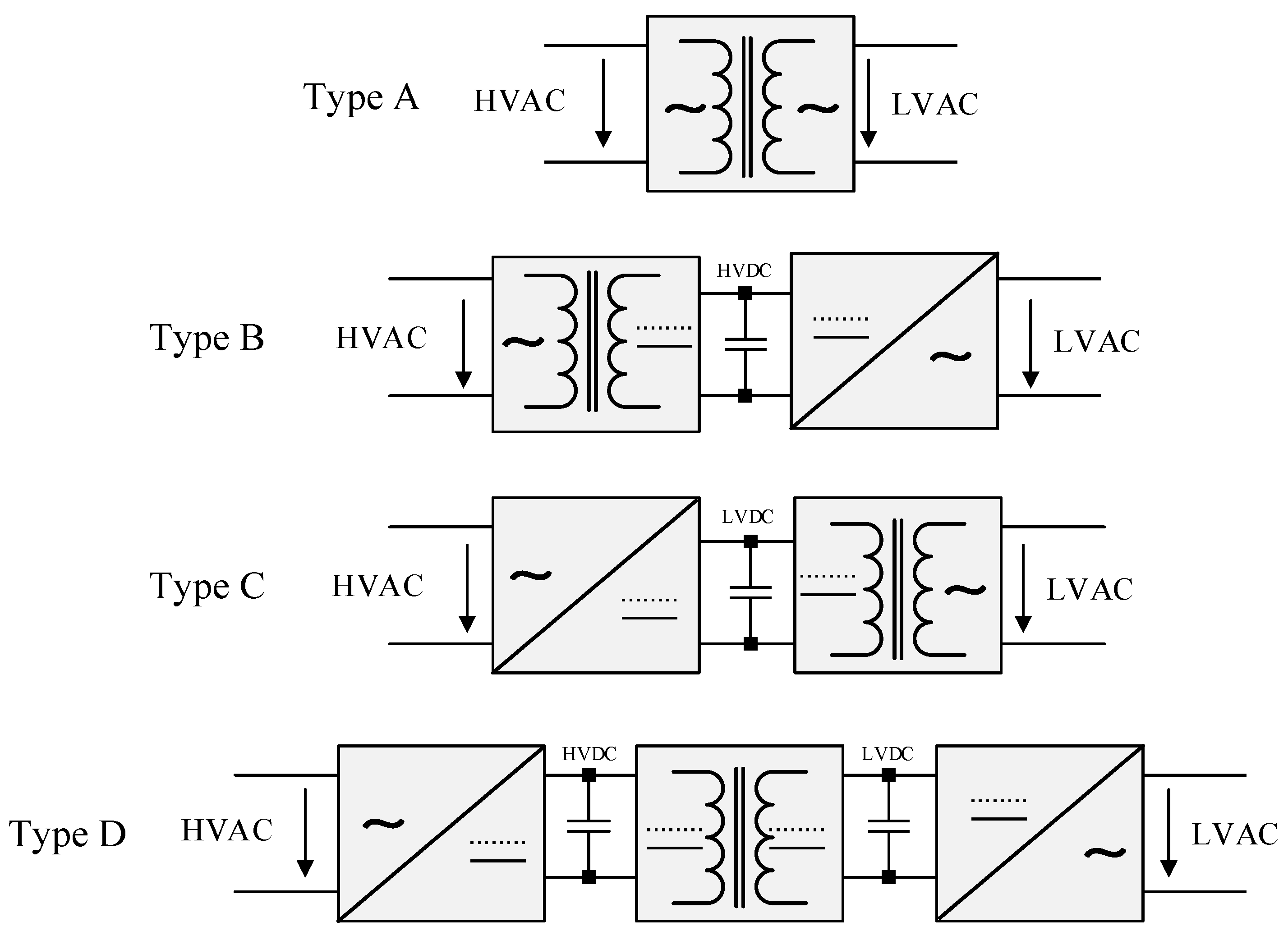
2.1. Solid-State Transformer

The SST can assume several topologies; some examples are given in Figure 1. The main difference between the various topologies is the number of constituent stages, the availability of direct current (DC) buses, the allowed functions, and the control complexity [1,18].

The three-stage topology, Type D, has the greatest popularity due to its features such as reactive power compensation, voltage drop compensation, integration of renewable energy sources, and integration with energy storage systems, among others. It is designed to provide two DC buses, a low voltage (LV), and a high voltage (HV), which allow the integration of other components to improve the power quality or to supply direct current equipment. The main disadvantage of this topology is the large number of power semiconductors required, which generally translates into lower efficiency and lower reliability [18,19].

In all the topologies depicted in Figure 1, power bidirectionality can be ensured by using power semiconductors that support operation in all four quadrants. The topology of the transformer is as important as the components in meeting the requirements of power density and efficiency. As SST applications, we highlight the solenoidal structures, namely the core type, shell type, and matrix type in Figure 2 [2,18].

The main advantage of the core type is that the windings are around a single magnetic core, which results in a weight reduction of the transformer [2]. However, a large part of the magnetic core is surrounded by windings, which, associated with the poor thermal conductivity of the magnetic core, become a disadvantage of the core type and consequently an advantage of the shell type from a thermal point of view. Apparently, the matrix type has the same advantages as the shell type, but it has two major disadvantages that restrict its use: first, the number of magnetic cores, which results in the increased volume and weight of the transformer and, consequently, increased losses and cost; second, the primary and secondary are separated at opposite ends of the magnetic core, leading to higher leakage inductance, an unfavorable quality in large power converters [2].

The main challenge in the design of conductors for high frequency operation is the effect of eddy currents in the windings and their contributions to system losses, namely, the losses due to skin effect and proximity effect, outlined as follows:

• Skin effect: the passage of an alternating current through a conductor causes a time-varying magnetic field, which, according to Faraday’s law, causes an electric field. The electric field induces eddy currents in the conductor, which oppose the variation in current density. The combination of the magnetic field and the induced electric field, both time-varying, creates electromagnetic induction in the conductor. This forces most of the electric current to flow at the surface of the conductor, instead of flowing uniformly. The skin effect is aggravated with increased operating frequency [20,21];
• Proximity effect: when two conductors close to each other are crossed by an alternating current, the current distribution in each conductor is affected by the changing magnetic field of the other conductor. Due to the induced eddy currents, the current will flow in undesired patterns, and this effect is also aggravated with increasing frequency [20,21].

Ultimately, these effects can also be interpreted as increases in the resistivity of the conductor as the frequency increases.

Of the mechanisms developed so far, the most efficient for reduction is the Litz wire. This consists of a set of single conductors isolated from each other, which can also be braided together in a uniform pattern, as illustrated in Figure 3 [22].

For a given application, there is not just one ideal conductor topology. The best solution will depend on the objectives, e.g., minimization of volume, minimization of losses, or minimization of costs. Determining the best conductor topology for a given application requires calculation methods, as in [20].

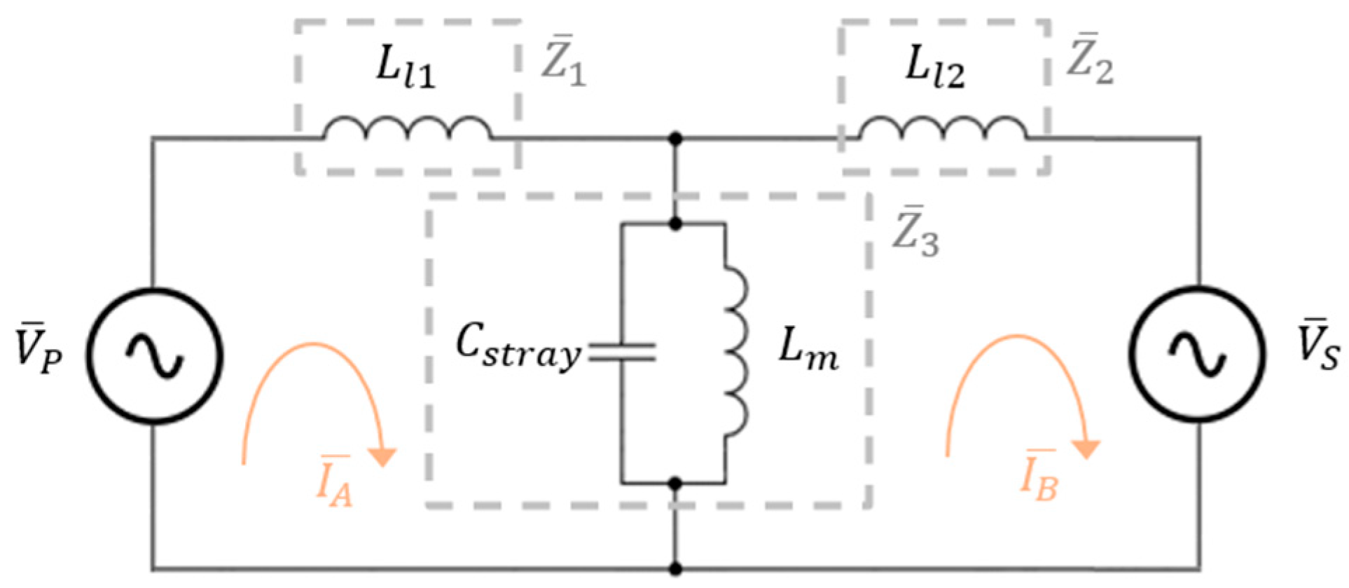
2.2. Transformer Modeling

Over the last decades, the trend has been to increase the power and frequency (typically from some kHz to dozens of MHz) of magnetic circuits. Nevertheless, this leads to a challenging design of magnetic circuits where parasitic effects play a key role. According to [23,24], most of the proposed designs are based on optimization routines, depending on the temperature rise and assuming uniform heat dissipation. Some authors consider the desired efficiency as a design input for the HFT [24]; otherwise, the optimization is focused on the A_p area [25,26]. In [27], the magnetizing inductance is considered the first step for the design process of HFT. In [28], The leakage inductance is first investigated, and then the remaining parameters of HFT are given.

This paper proposes a step-by-step methodology for designing medium and high-frequency transformers and their optimum electrical and magnetic specifications to reduce volume and increase efficiency. The proposed design methodology for the HFT first finds the optimum magnetic- flux density and then arrives at the other parameters according to the desired criteria such as leakage inductance and losses, as shown in Figure 4.

• System and Topology Specifications: Definition of the main system specifications, namely: apparent power ($S$), primary voltage ($V_P$), secondary voltage ($V_S$), operating frequency (f), ambient temperature ($T_a$), admissible temperature variation (ΔT), wave factor ($K_v$), window utilization factor ($k_u$) and stacking factor ($k_f$);
• Magnetic Core Properties: Selection of the material to be used for the magnetic core to find the saturation flux density ($B_{sat}$) and parameters of the constants α, β and Kc of the respective material, essential parameters for the following steps; most common cores, such as amorphous, ferrite, and nanocrystalline magnetic materials are compared in [29] for core losses at 10, 20, 50, and 100 kHz, respectively.
• Calculate Optimum Flux Density: The optimal flux density corresponds to the flux density value that minimizes the sum of copper losses with iron losses. Knowing the expression that describes the losses in copper and iron, as a function of the frequency and flux density, and after numerical simplification, it is possible to obtain the expression of the optimal flux density by Equation (1), as laid out in [30].

$$B_{opt}=\frac{{\left(h_c k_a ∆T\right)}^{\frac{2}{3}}}{{2^{\frac{2}{3}}\left({\rho }_w k_w k_u\right)}^{\frac{1}{12}}{\left(k_c K_c f^{\alpha }\right)}^{\frac{7}{12}}}{\left(\frac{K_V f k_f k_u}{\sum VA}\right)}^{\frac{1}{6}}$$

(1)

where $k_a$, $k_c$, $k_w$ are dimensionless constants, which usually assume the values $40$, $5.6$ and $10$ respectively [30]; $\sum VA$ represents the apparent power of the transformer, $h_c$ is the heat transfer coefficient, and ${\rho }_w$ is the electrical resistance of the conductor that composes the windings.

4.

Magnetic Core Sizing: For the optimal flux density, determined in the previous point, the dimensions of the magnetic core of the transformer are selected based on the product of the window area ($W_a$) by the cross-sectional area ($A_c$); this product is given the nomenclature $A_p$, usually expressed in ${\mathrm{c}\mathrm{m}}^4$. For the analytical determination of this parameter, it is necessary to perform a comparison between the value of the optimal flux density ($B_{opt}$) and the saturation flux density value ($B_{sat}$). Based on the exposition in [30]:

• If $B_{opt}<B_{sat}$, the value of the parameter $A_p$ is given by Equation (2).

$$A_p={\left(\frac{\sqrt{2} \sum VA}{K_V f B_{opt} k_f K_t \sqrt{k_u ∆T}}\right)}^{\frac{8}{7}}$$

(2)

• If $B_{opt}>B_{sat}$, the value of the parameter $A_p$ is given by Equation (3).

$$f\left(A_p\right)=a_0 {A_p}^2-a_1 {A_p}^{\frac{7}{4}}+a_2$$

(3)

where the parameters $a_0$, $a_1$ and $a_2$ are given by Equations (4), (5) and (6) respectively [30].

$$a_0=\frac{k_c K_c f^{\alpha } B_{max}^{\beta }}{{\rho }_w V_w k_u}$$

(4)

$$a_1=\frac{h_c k_a ∆T}{{\rho }_w k_w k_u}$$

(5)

$$a_2={\left(\frac{\sum VA}{K_V f B_{sat} k_f k_u}\right)}^2$$

(6)

Based on the determined analytical value, $A_p$, a magnetic core with an equal or greater value should be chosen.

5.

Calculate the Number of Turns: The number of turns of each winding can be described by Equation (7).

$$N=\frac{V_{rms}}{K_v B_{max} A_m f}$$

(7)

where the parameter $A_m$ represents the effective cross-sectional area of the core, which is given by the product between the physical cross-sectional area of the core ($A_c$) and the staking factor ($k_f$) [17,30].

6.

Conductor Sizing: For the dimensioning of the conductors to be used it is necessary to determine the current density ($J_o$). To determine this parameter, it is necessary to compare the value of the optimum flux density ($B_{opt}$) and the value of the saturation flux density ($B_{sat}$). Based on [30]:

• If $B_{opt}<B_{sat}$, the value of $J_o$ is given by Equation (8).

$$J_o=K_t \sqrt{\frac{\mathsf{\Delta }T}{2k_u}} \frac{1}{\sqrt[8]{A_p}}$$

(8)

• If $B_{opt}>B_{sat}$, the value of $J_o$ is given by Equation (9).

$$J_o=\sqrt{\frac{h_c k_a A_p^{\frac{1}{2}} ∆T-V_c K_c f^{\alpha } B_{sat}^{\beta }}{{\rho }_w V_w k_u}}$$

(9)

For parameter $A_p,$ the value of the previously chosen magnetic core should be used. Where the parameters $V_c$, $V_w$ represent the volume of the core and the volume of the windings respectively, these parameters can be calculated from Equations (10) and (11), respectively. Where $l_c$ is the average length of the magnetic part of the core, $MLT$ is the average length of a coil, and $W_a$ is the area of the magnetic core window.

$$V_c=l_c A_c$$

(10)

$$V_w=MLT W_a$$

(11)

The l_c and MLT length can be obtained using Equations (12) and (13) respectively, where dimensions a, b, d, f and u are obtained from the core dimensions, as in Figure 5.

$$l_c=f+u+\left(a+b\right)$$

(12)

$$MLT=2\left(\frac{b}{4}+a+\frac{b}{4}\right)+2\left(\frac{b}{4}+d+\frac{b}{4}\right)$$

(13)

To minimize the skin effect and the proximity effect, the choice of the Litz wire should consider the previously determined current density. However, the sizing of the internal structure of the Litz wire is highly complex. In [20,31], simplified methods for sizing Litz wire are presented. In this study, we used the data provided by the manufacturers, namely the relationship between section/number of single conductors and the type of construction.

7.

Estimation of Leakage Inductance: The estimation of leakage inductance can be obtained through Dowell’s model, but this model was designed to calculate the leakage inductance in a transformer composed of foil conductor windings. Considering that the model under study uses Litz wire windings, it will first be necessary to perform the equivalence between Litz wire and foil conductors and subsequently estimate the leakage inductance value through Dowell’s model.

The thickness of a sheet conductor, $d_{eq}$, may be given by Equation (14), where $d$ represents the diameter of each conductor that makes up the Litz wire. For the height of the foil winding, it will be considered that it occupies the entire height of the window, a situation that will allow simplification of the calculation. The equivalent section can be given by Equation (15), where $h_w$ and $d_w$ represent, respectively, the height and width of the winding composed of Litz conductors. Thus, the number of sheet conductors, m, will be given by Equation (16), where $N$ represents the number of turns of each winding, and $n$ represents the number of single conductors that make up the Litz wire [32].

$$d_{eq}=d\sqrt{\frac{\pi }{4}}$$

(14)

$$K_w=\frac{h_w}{d_w}$$

(15)

$$m=\sqrt{\frac{N n}{K_w}}$$

(16)

Using Dowell’s model, the estimate of the leakage inductance, referenced to the primary, is given by Equation (17). Where $d_g$ is the distance between windings and $d_i$ is the distance between consecutive sheet conductors. The indices “1” refer to the primary and the indices “2” refer to the secondary of the HFT [30,31,32,33].

$$L_l=\mu {N_1}^2\frac{MLT}{h_{eq}}\left[d_{{eq}_1}\frac{m_1}{3}{F}_{L_1}+d_{{eq}_2}\frac{m_2}{3}{F}_{L_2}+d_g+d_{i_1}\frac{\left(m_1-1\right)}{2m_1}+d_{i_2}\frac{\left(m_2-1\right)}{2m_2}\right]$$

(17)

The inductance factor, $F_L$, is given by Equation (18). The parameter $\mathsf{\Delta }$ is given by the ratio between the thickness of the sheet conductor, $d_{eq}$, and the skin effect, $\delta$, using Equations (19) and (20).

$$F_L=\frac{1}{2 m^2 \mathsf{\Delta }}\left[\left(4m^2-1\right) {\phi }_1-2 \left(m^2-1\right) {\phi }_2\right]$$

(18)

$${\phi }_1=\frac{\sinh \left(2\mathsf{\Delta }\right)-\sin \left(2\mathsf{\Delta }\right)}{\cosh \left(2\mathsf{\Delta }\right)-\cos \left(2\mathsf{\Delta }\right)}$$

(19)

$${\phi }_2=\frac{\sinh \left(\mathsf{\Delta }\right)-\sin \left(\mathsf{\Delta }\right)}{\cosh \left(\mathsf{\Delta }\right)-\cos \left(\mathsf{\Delta }\right)}$$

(20)

8.

Core and Winding Losses and Efficiency: The power losses in the iron can be translated by (21), and the value obtained by this equation will be expressed in W/m³ [30,34].

$$P_{fe}={k_i \left|∆B\right|}^{\beta } \frac{1}{T^{\propto }}\left[D^{1-\propto }+{\left(1-D\right)}^{1-\propto }\right]$$

(21)

where the parameter $k_i$ is given by Equation (22), the parameter $T$ represents the period (inverse of the operating frequency), the parameter $D$ represents the cycle factor, and the parameter $∆B$ represents the flux density variation.

$$k_i=\frac{K_c}{2^{\beta -1} {\pi }^{\alpha -1}\left(1.1044+\frac{6.8244}{\alpha +1.354}\right)}$$

(22)

Particularizing for the case where a Dual Active Bridge, a DAB converter with a Dual Phase Shift (DPS) modulation technique is used, the variation of the flux density ($∆B$), could be translated by twice the maximum flux density ($B_{max}$), where the maximum flux density is given by Equation (23) [30,34].

$$B_{max}=\frac{\sqrt{D} V_{DC}}{K_V f N_p A_c}$$

(23)

The power losses in each winding, considering the harmonic components of the current, can be translated by Equation (24) [30].

$$P_{cu}=R_{DC} {I_{DC}}^2+\sum _{n=1}^{\infty }{R}_{{AC}_n} {I_n}^2$$

(24)

The parameter $I_{DC}$ represents the value of the direct current, and the parameter $I_n$ represents the value of the alternating current for harmonic $n$. It is also necessary to know the value of the DC resistance ($R_{DC}$) and the value of the AC resistance ($R_{AC}$); the latter also depends on the frequency of the harmonic. The value of the DC resistance can be given by Equation (25), where $\rho$ is the electrical resistance of the conductor.

$$R_{DC}=\frac{2 \rho m MLT}{h_{eq} d_{eq}}$$

(25)

The value of the AC resistance, for harmonic n, based on Dowell’s equation is given by Equation (26). It is designed to foil type windings, so the power losses in the windings will be calculated for the equivalent foil winding determined in Topic 7 [35].

$$R_{AC}=R_{DC} A_{str}\sqrt{n}\left(\frac{\sinh \left(2A_{str}\sqrt{n}\right)+\sin \left(2A_{str}\sqrt{n}\right)}{\cosh \left(2A_{str}\sqrt{n}\right)-\cos \left(2A_{str}\sqrt{n}\right)}+\frac{2\left({N_l}^2-1\right)}{3}\frac{\sinh \left(A_{str}\sqrt{n}\right)-\sin \left(A_{str}\sqrt{n}\right)}{\cosh \left(A_{str}\sqrt{n}\right)+\cos \left(A_{str}\sqrt{n}\right)}\right)$$

(26)

The term $A_{str}$ is described by Equation (27), which results from the ratio between sheet conductor thickness, $d_{eq}$, and the skin effect, $\delta$, for the operating frequency [35].

$$A_{str}=\frac{d_{eq}}{\delta }$$

(27)

The efficiency of HFT can be determined by (28).

$$\eta =\frac{P_{out}}{P_{out}+P_{fe}+P_{cu}}$$

(28)

In HFTs, the accounting of parasitic parameters, namely parasitic capacitances, is fundamental for the correct modeling of the system. These capacitances are responsible for unwanted resonance frequencies and oscillations of the temporal evolution of the current and consequently a decrease in the reliability and efficiency of the system.

The parasitic capacitances in a winding are essentially between conductors of the same winding, of different windings, and between the conductors and the magnetic core. The three factors with the greatest contribution to the value of the parasitic capacitance are the dielectric constant of the insulating materials used, conductor geometry (diameter and size of the conductor, space between conductors and their distance from the magnetic core) and the characteristics of the winding (organization of conductors and winding direction) [36,37].

The following calculates the equivalent parasitic capacity, as described in [36,37,38,39].

The equation for determining the $C_{stray}$ is given by Equation (29), based on the equivalent circuit of six capacitors and the simplification to a single equivalent capacitance [38].

$$C_{stray}=C_{P_1}+k^2 C_{S_1}+2k \left(\frac{C_{S_3}{C}_{P_3}-C_{P_2}{C}_{S_2}}{C_{P_2}+C_{S_3}+C_{P_3}+C_{S_2}}\right)+\left(\frac{\left(C_{S_3}+C_{P_2}\right)\left(C_{P_3}+C_{S_2}\right)+k^2\left(C_{P_2}+C_{P_3}\right)\left(C_{S_3}+C_{S_2}\right)}{C_{P_2}+C_{S_3}+C_{P_3}+C_{S_2}}\right)$$

(29)

The equivalent resistance of the transformer’s magnetic core, $R_c$, can be described by Equation (30), in which $l_m$ represents the average length that the magnetic flux describes in the magnetic core [40].

$$R_c=\frac{l_m}{{\mu }_o {\mu }_r A_c}$$

(30)

The equivalent inductance of the magnetic core of the transformer, $L_m$, can be by Equation (31) [17].

$$L_m={\mu }_o {\mu }_r {N_p}^2 \frac{A_c}{l_m}$$

(31)

Figure 6 shows the simplified equivalent scheme of an HFT, referenced to the transformer’s primary [41]. With the transition of a parameter from the secondary to the primary, as a rule, the same nomenclature is maintained, but a pellicle is added.

2.3. Converter Modeling

Based on the HFT modeling exposed above, it is possible to model the converter under study. Figure 7 represents the simplified power and control scheme, consisting of a Type D SST (see Figure 1), the only one between the two DC buses, that are the target of this study.

The schematic depicted in Figure 7 also corresponds to the structure of a DAB, consisting of two single phase bridges, connected to each other via an HFT. To allow power bidirectionality, the semiconductors should be fully controllable, e.g., IGBT or MOSFET. Several control techniques can e used, which are described in more detail in [42,43]. For the present study, rectangular modeling was used and is described below [42].

3. Control System

The implemented output voltage control establishes a phase shift angle control between the primary and secondary voltage waveforms, which is only applied to the second converter of the DAB. The first converter of the DAB assumes a null angle and is constant over time [42].

The purpose of the phase shift angle control is to regulate the power delivered to the load so that the voltage at the load terminals assumes a constant and predefined value, regardless of the load power, considering the power limitations supported by the system. Thus, the phase shift angle is determined by measuring the voltage at the load terminals.

Figure 8 presents the block diagram of the controller. The power converter is modulated with a gain, $K_d$, a delay time, $T_{d,}$ and the load dynamics. Subtracting the reference voltage, $V_{0_{Ref}}$, from the measured voltage at the output of the converter, $V_0$, provides the value of the voltage error. The gain $\alpha$ depends on the configuration of the instrumentation used to perform the output voltage measurement, and for simulation purposes this parameter is assumed to be a unitary.

The controller $C\left(s\right),$ has as output the phase shift angle, given by $\sin \left(\delta \right)$, allows a zero error to be obtained, so that the output voltage, $V_0$, assumes the value of the reference voltage, $V_{0_{Ref}}$.

Based on the simplified equivalent circuit of the HFT, represented in Figure 9, where ${\stackrel{-}{V}}_P$ and ${\stackrel{-}{V}}_S$ represent the voltage at the primary and secondary terminals, respectively, performing the mesh analysis and after algebraic simplification, it is possible to obtain Equation (32).

$${\stackrel{-}{I}}_P=\frac{Z_3 V_S\sin \left(\delta \right)}{A}-\left(\frac{Z_3 V_S\cos \left(\delta \right)+\left(Z_3+Z_2\right) V_P}{A}\right)j$$

(32)

To design the controller C(s), it is necessary to establish the relationship between the input power of the DAB converter, $P_{in}$, and the output power of the DAB converter, $P_0$, which corresponds to the power delivered to the load. Assuming that the converter is ideal, to simplify the controller design, i.e., that the input power is equal to the output power, it is possible to derive the expressions exposed in Equation (33).

$$P_0=P_{in}=Re\left({\stackrel{-}{V}}_P {\stackrel{-}{I}}_P\right)\to V_0=\frac{Z_3 V_P V_S\sin \left(\delta \right)}{A I_0}$$

(33)

Since the controller $C$(s) outputs $\sin \left(\delta \right),$ and based on the equivalent controller scheme depicted in Figure 8, it is possible to conclude that the gain $K_d$ will be given by Equation (34).

$$K_d=\frac{Z_3 V_P V_S}{A I_0}$$

(34)

Considering the use of a proportional integral (PI) controller, starting from the diagram represented in Figure 8, consider $\alpha =1$ and cancelling the dominant pole with the controller zero, it is possible to obtain the closed chain transfer function, represented in Equation (35).

$$\frac{V_0 \left(s\right)}{V_{0_{ref}} \left(s\right)}=\frac{\frac{K_c}{s} \frac{K_d}{1+s{T}_d}}{1+\frac{K_c}{s} \frac{K_d}{1+s T_d}}$$

(35)

By simplifying Equation (35) and comparing it with the canonical second-order equation, it is possible to determine the expressions that define the proportional and integral gain, represented in Equations (36) and (37) [44], respectively.

$$K_I=\frac{{{\omega }_o}^2 T_d}{K_d R}$$

(36)

$$K_P=\frac{{{\omega }_o}^2 T_d}{K_d R} {\tau }_c$$

(37)

4. Simulation Results

4.1. Introduction

The application under study consists in supplying a fast charger of an electric vehicle from the electrical network provided by the energy distributors. Furthermore, it is assumed that there is power bidirectionality. Figure 10 shows the generic block diagram that summarizes the various elements inherent to the application.

The present study focuses only on the “Module”, which consists of the two converters and the HFT, as represented generically in Figure 7. The main considerations assumed are as follows:

• “Three-phase bridge rectifiers”, fed from the conventional three-phase grid (400 V 50 Hz), composed of fully controlled semiconductors. For simulation purposes, consider an ideal DC voltage source of equal effective value;
• To simplify the analysis, the power requested by the “Charger/Battery” will be considered as a pure resistive load with equal power value. Consider that the charger should be powered with 1000 V DC.

Based on the flowchart presented in Figure 4 and the above considerations,

Table 2. Main dimension parameters.

	Parameter	Value
$S$	Apparent power	$50 \mathrm{k}\mathrm{V}\mathrm{A}$
$V_P$	Effective voltage applied to the primary	$530 \mathrm{V}$
$V_S$	Effective voltage applied to the secondary	$1 \mathrm{k}\mathrm{V}$
$f$	Operating frequency	1 kHz
$\mathsf{\Delta }T$	Admissible temperature variation	$35.0 °\mathrm{C}$
	Magnetic core: core type, amorphous material, manufacturer Transmart, model CACC-3604	---
$B_{Sat}$	Saturation flux	$1.56 \mathrm{T}$
$B_{Opt}$	Optimum saturation flux	$0.59 \mathrm{T}$
$A_P$	Value concerning the model CACC-3604	$3563.5 {\mathrm{c}\mathrm{m}}^4$
kf	Stacking factor	0.9
$N_P$	Number of primary coils	$33$
$N_s$	Number of secondary windings	$61$
$J_0$	Current density	0.81 A/mm2

and

Table 3. Constitution of the windings.

Primary Winding: Litz Wire
№ of Single Conductors	$1368$
Construction	$12\times \left(3\times \frac{38}{0.08} {\mathrm{m}\mathrm{m}}^2\right)$
Equivalent Copper Section	$120 {\mathrm{m}\mathrm{m}}^2$
Secondary Winding: Litz Wire
№ of Single Conductors	$840$
Construction	$6\times \left(5\times \frac{24}{0.08} {\mathrm{m}\mathrm{m}}^2\right)$
Equivalent Section	$70 {\mathrm{m}\mathrm{m}}^2$

show the main dimensioned parameters.

For the constitution of the windings, we used the characteristics of the conductors provided by the manufacturer New England Wire Technologies. The size of the windings must be compatible with the size of the magnetic core chosen; Table 3 summarizes this.

For the previous data, we obtain a value of theoretical power losses in the iron of $98.5\mathrm{W}$ and in the copper of $526.5\mathrm{W}$, for calculation purposes until the 13th harmonic. This results in a theoretical efficiency of $98.8\mathrm{\%}$.

The parameters of the HFT, which respond to the equivalent scheme presented in Figure 6, are shown in

Table 4. The HFT equivalent parameters.

Parameter	Value
$R_1$	$17.01 \mathrm{m}\mathsf{\Omega }$
$L_{l1}$	$34.26 \mathsf{\mu }\mathrm{H}$
${L^{\prime }}_{l2}$	$10.37 \mathsf{\mu }\mathrm{H}$
${R^{\prime }}_2$	$5.30 \mathrm{m}\mathsf{\Omega }$
$C_{stray}$	$0.40 \mathrm{n}\mathrm{F}$
$R_c$	$18.55 \mathrm{k}\mathsf{\Omega }$
$L_m$	$58.70 \mathrm{m}\mathrm{H}$
$C_{add}$	$1.00 \mathrm{m}\mathrm{F}$
$L_{add}$	$80.00 \mathrm{m}\mathrm{H}$

. The need to add a capacitor in parallel with the load and an inductance in series with the transformer were verified to improve the behavior/performance of the controller and consequently of the system to be modeled.

4.2. Numerical Simulation Results

To verify the performance of the scaled transformer model and the ability of the control to adapt, three tests were employed:

• Test 1—Constant Load: Consider that the system feeds a constant, purely resistive load in the direct power direction and that the load has a power of 50 kVA.

By analyzing the waveforms of the voltage represented in Figure 11, it is possible to verify that the control system worked as expected, acting on the phase shift angle so that the voltage at the load terminals assumes the previously established reference value. The value of the phase shift angle depends essentially on the equivalent inductance of the model under study and the value of the current that the load requests, having as a maximum value $+\mathsf{\Omega }/2$.

To evaluate the performance of the developed HFT, its performance can be analyzed. Figure 11 represents the average instantaneous power at the primary and secondary terminals. By using the measurement tools integrated in the software, Matlab/Simulink, it is possible to determine the obtained efficiency, having verified a value of $99.5\mathrm{\%}$. Analyzing the obtained efficiency, we conclude that it does not consider the winding resistance variation as a function of frequency and does not account for the skin effect. When the theoretical efficiency is determined without accounting for the skin effect, a theoretical efficiency of $99.4\mathrm{\%}$ is obtained.

The analysis of the voltage waveform at the transformer terminals will be performed in Test 3.

• Test 2—Variable load: Consider that the system is feeding a variable load, purely resistive, in the direct power direction. The initial load presents a power of $25\mathrm{kVA}$ and, at instant $t=1\mathrm{s}$ the load doubles, resulting in a power of $50\mathrm{kVA}$. All the analysis performed for Test 1 is valid for Test 2. The focus of the analysis described below is the impact of varying the value of the load on the system under study.

Analyzing Figure 12 it is possible to verify the occurrence of a voltage drop at the load terminals and a consequent controller action to guarantee the reference voltage at the load terminals. The voltage drop is significant, but it should be considered that the instantaneous doubling of the load is an extremely demanding transient for the system. Nevertheless, it is an excellent case to test the good performance of the controller. The shift angle after load variation and stabilization assumes approximately twice the value because the load has also doubled from $25\mathrm{k}\mathrm{V}\mathrm{A}$ to $50\mathrm{k}\mathrm{V}\mathrm{A}$.

Figure 12 shows the variation of the average instantaneous power at the HFT terminals. Although this is a different test, after the stabilization of the load of $50\mathrm{k}\mathrm{V}\mathrm{A}$, the performance values verified are the same as those in Test 1. When the load assumes a value of $25\mathrm{k}\mathrm{V}\mathrm{A}$, an efficiency in simulation of $99.7\mathrm{\%}$ is verified.

• Test 3—Power Bidirectionality: Consider that the system is supplying a purely resistive load with a power of $50\mathrm{kVA}$ in the direct power direction, and at instant $t=1\mathrm{s}$, the power flow changes from the direct direction to the reverse direction, at which point the load is supplying the grid with a power of $50\mathrm{kVA}$.

The shift angle is only applied to the bridge on the secondary side of the HFT, operating the bridge on the primary side of the HFT with a zero angle. When the power flow switches from the forward to the reverse direction, the phase shift angle will have to take on a negative value, as verified in Figure 13.

Figure 12 also shows the variation of the average instantaneous power at the transformer terminals, where it is possible to see the power bidirectionality. The efficiency verified when the power flow is in the direct direction is equal to the efficiency described in Test 1. When the power flow is in the reverse direction, the same efficiency value is verified, $99.5\mathrm{\%}$, and in this instance, the value of the average instantaneous power in the secondary is higher than the value of the average power in the primary. This allows the conclusion that regardless of the power flow direction, for the same power value, the losses in the transformer will be approximately equal.

The temporal evolutions of the voltage at the load terminals present the same temporal progression as described in Tests 1 and 2.

The impact of the variation of the shift phase angle can also be seen in Figure 14, where the temporal evolution of the voltage at the HFT terminals is represented. When the power flow is in the forward direction, the secondary voltage leads the primary voltage. On the contrary, when the power flow is in the opposite direction, it is verified that the secondary voltage is laggs the primary voltage.

5. Conclusions

SST’s are increasingly used to replace traditional transformers (50/60 Hz) because of the many advantages they provide, such as smaller dimensions, higher power density, ease of integration with alternative systems, supply of loads in direct current, and integration of systems for the improvement of power quality, among others. However, utilizing HFTs instead of low frequency transformers may present higher costs because numerous power components and auxiliary control circuits are required, which can be relatively complex and expensive.

Several simulation tests were performed in Matlab/Simulink on the application of the SST to a fast charger of an electric vehicle supplied by an electrical network. In these simulation tests, an efficiency of around $99.5\mathrm{\%}$ was obtained for a 50 kVA constant resistive load operating at 1 kHz. Another test was also performed, in which the load was changed from 25 kVA to 50 kVA. Despite the extreme load variation, the controller presented good performance and fast stabilization. The maximum efficiency was 99.7% obtained at 25 kVA. The bidirectionality power flow of the solution was also tested and confirmed, showing a gradual transition from battery charging (Grid-to-Vehicle—G2V) to battery discharging (Vehicle-to-Grid—V2G) while the phase shift angle changed from positive to negative values to regulate the power delivered to the load.

According to the simulation results obtained, all our objectives were verified, such as the validation of the theoretical model of the HFT, the validation of the control scheme developed for SST control, and the verification of the ability to support power bidirectionality. Furthermore, temporal evolutions and efficiency values consistent with the theoretical concepts were obtained.

References

1. Hannan, M.A.; Ker, P.J.; Lipu, M.S.H.; Choi, Z.H.; Muttaqi, K.M.; Blaabjerg, F. State of the Art of Solid-State Transformers: Advanced Topologies, Implementation Issues, Recent Progress and Improvements. IEEE Access 2020, 8, 19113–19132. [Google Scholar] [CrossRef]
2. Agheb, E.; Høidalen, H.K. Medium Frequency High Power Transformers, State of Art and Challenges. In Proceedings of the 2012 International Conference on Renewable Energy Research and Applications (ICRERA), Nagasaki, Japan, 11–14 November 2012. [Google Scholar] [CrossRef]
3. Joshi, A.; Nath, S. Effect of High-Frequency Transformer Parasitic Capacitances on Operation of Solid-State Transformers. In Proceedings of the 2022 Second International Conference on Power, Control and Computing Technologies (ICPC2T), Raipur, India, 1–3 March 2022; pp. 1–6. [Google Scholar] [CrossRef]
4. Olowu, T.O.; Jafari, H.; Moghaddami, M.; Sarwat, A.I. Physics-Based Design Optimization of High Frequency Transformers for Solid State Transformer Applications. In Proceedings of the 2019 IEEE Industry Applications Society Annual Meeting, Baltimore, MD, USA, 29 September–3 October 2019; pp. 1–6. [Google Scholar] [CrossRef]
5. Rashidi, M.; Bani-Ahmed, A.; Nasiri, R.; Mazaheri, A.; Nasiri, A. Design and implementation of a multi winding high frequency transformer for MPSST application. In Proceedings of the 2017 IEEE 6th International Conference on Renewable Energy Research and Applications (ICRERA), San Diego, CA, USA, 5–8 November 2017; pp. 491–494. [Google Scholar] [CrossRef]
6. Peng, Z.; Wang, G.; Zhai, X.; Zhang, X.; Zhou, H.; Yi, C. Optimum Design of High Frequency Transformer Based on Winding Spacing. In Proceedings of the 2019 22nd International Conference on Electrical Machines and Systems (ICEMS), Harbin, China, 11–14 August 2019; pp. 1–6. [Google Scholar] [CrossRef]
7. Guo, S.; Liu, P.; Zhang, L.; Huan, A.Q. Design and optimization of the high frequency transformer for a 800V/1.2MHz SiC LLC resonant converter. In Proceedings of the 2017 IEEE Energy Conversion Congress and Exposition (ECCE), Cincinnati, OH, USA, 1–5 October 2017; pp. 5317–5323. [Google Scholar] [CrossRef]
8. Wen, H.; Liu, Y.; Jiao, D.; Yeh, C.-S.; Lai, J.-S. Design Principles and Optimization Considerations of a High Frequency Transformer in GaN Based 1 MHz 2.8 kW LLC Resonant Converter with over 99% Efficiency. In Proceedings of the 2021 IEEE Applied Power Electronics Conference and Exposition (APEC), Phoenix, AZ, USA, 14–17 June 2021; pp. 1939–1944. [Google Scholar] [CrossRef]
9. Di Noia, L.P.; Rizzo, R. Comparison Between Different High-Frequency Transformer for Resonant Power Converter. In Proceedings of the 2022 IEEE 16th International Conference on Compatibility, Power Electronics, and Power Engineering (CPE-POWERENG), Birmingham, UK, 29 June–1 July 2022; pp. 1–5. [Google Scholar] [CrossRef]
10. Kawaguchi, Y.; Furukawa, K.; Shimada, T.; Kusukawa, J. Feasibility Study of High-Frequency Transformer with High-Voltage Insulation Structure for SST Based Medium-Voltage Multi-Level Converter. In Proceedings of the 2022 International Power Electronics Conference (IPEC-Himeji 2022-ECCE Asia), Himeji, Japan, 15–19 May 2022; pp. 1769–1774. [Google Scholar] [CrossRef]
11. Zhao, B.; Song, Q.; Li, J.; Xu, X.; Liu, W. Comparative Analysis of Multilevel-High-Frequency-Link and Multilevel-DC-Link DC–DC Transformers Based on MMC and Dual-Active Bridge for MVDC Application. IEEE Trans. Power Electron. 2018, 33, 2035–2049. [Google Scholar] [CrossRef]
12. Grzejszczak, P.; Wolski, K.; Brzostek, K.; Sitnik, A. Comparative study of two types of high-frequency transformers in a 20-kW Phase-Shifted Full Bridge converter application. In Proceedings of the 2022 Progress in Applied Electrical Engineering (PAEE), Koscielisko, Poland, 27 June–1 July 2022; pp. 1–4. [Google Scholar] [CrossRef]
13. Chen, L.; Zhang, Z.; Wang, X.; Fu, Q.; Xing, Z. Analysis of Electromagnetic Characteristics of High Frequency Transformer Based on C Type Nanocrystalline Magnetic Core. In Proceedings of the 2019 11th International Conference on Measuring Technology and Mechatronics Automation (ICMTMA), Qiqihar, China, 28–29 April 2019; pp. 132–135. [Google Scholar] [CrossRef]
14. Cao, Z.; Chen, W.; Jiang, J.; Zhang, K.; Chen, Y.; Shen, Z. Design of Dry-type High-power High-frequency Transformer Based on Triangular Closed Core. In Proceedings of the 2021 IEEE Sustainable Power and Energy Conference (iSPEC), Nanjing, China, 23–25 December 2021; pp. 3336–3341. [Google Scholar] [CrossRef]
15. Djuric, S.; Stojanovic, G.; Damnjanovic, M.; Radovanovic, M.; Laboure, E. Design, Modeling, and Analysis of a Compact Planar Transformer. IEEE Trans. Magn. 2012, 48, 4135–4138. [Google Scholar] [CrossRef]
16. Barbini, N.; Colavitto, A.; Vicenzutti, A.; Contin, A.; Sulligoi, G. High Frequency Modeling of Foil Type Transformers for Shipboard Power Electronic Power Distribution Systems. In Proceedings of the 2019 AEIT International Annual Conference (AEIT), Florence, Italy, 18–20 September 2019; pp. 1–6. [Google Scholar] [CrossRef]
17. Elrajoubi, A.M.; Ang, S.S. High-Frequency Transformer Review and Design for Low-Power Solid-State Transformer Topology. In Proceedings of the 2019 IEEE Texas Power and Energy Conference (TPEC), College Station, TX, USA, 7–8 March 2019. [Google Scholar] [CrossRef]
18. She, X.; Burgos, R.; Wang, G.; Wang, F.; Huang, A.Q. Review of Solid State Transformer in the Distribution System: From Components to Field Application. In Proceedings of the 2012 IEEE Energy Conversion Congress and Exposition (ECCE), Raleigh, NC, USA, 15–20 September 2012. [Google Scholar] [CrossRef]
19. Falcones, S.; Mao, X.; Ayyanar, R. Topology Comparison for Solid State Transformer Implementation. In Proceedings of the IEEE PES General Meeting, Minneapolis, MN, USA, 25–29 September 2010. [Google Scholar] [CrossRef]
20. Sullivan, C.R. Optimal Choice for Number of Strands in a Litz-Wire Transformer Winding. IEEE Trans. Power Electron. 1999, 14, 283–291. [Google Scholar] [CrossRef] [Green Version]
21. Clement, C. Skin Effect in Electrical Conductors: Any Commercially Viable Solution; University of Aberdeen: Aberdeen, Scotland, 2014. [Google Scholar] [CrossRef]
22. McLyman, C.W.T. Transformer and Inductor Design Handbook; Kg Magnetics, Inc.: Idyllwild, CA, USA, 2004; ISBN 0-8247-5393-3. [Google Scholar]
23. Banumathy, J.R.; Veeraraghavalu, R. High Frequency Transformer Design and Optimization using Bio-inspired Algorithms. Appl. Artif. Intell. 2018, 32, 707–726. [Google Scholar] [CrossRef]
24. Zhang, S.; Chen, D.; Bai, B. Study of a High-Power Medium Frequency Transformer Using Amorphous Magnetic Material. Symmetry 2022, 14, 2129. [Google Scholar] [CrossRef]
25. Banumathy, J.R.; Veeraraghavalu, R. Optimal Design of Minimal Footprint High Frequency Transformer. Serb. J. Electr. Eng. 2021, 18, 303–320. [Google Scholar] [CrossRef]
26. Deepak, S.; Mohanrajan, S.R. High-Frequency Transformer design for a Bi-directional isolated DC-DC converter for Electric Vehicles. In Proceedings of the 2022 IEEE 7th International Conference on Recent Advances and Innovations in Engineering (ICRAIE), Mangalore, India, 1–3 December 2022; pp. 428–432. [Google Scholar] [CrossRef]
27. Dey, S.; Chakraborty, S.S.; Singh, S.; Hatua, K. Design of High Frequency Transformer for a Dual Active Bridge (DAB) Converter. In Proceedings of the 2022 IEEE Global Conference on Computing, Power and Communication Technologies (GlobConPT), New Delhi, India, 23–25 September 2022; pp. 1–6. [Google Scholar] [CrossRef]
28. Zhang, X.; Xiao, F.; Wang, R.; Kang, W.; Yang, B. Modeling and Design of High-Power Enhanced Leakage-Inductance-Integrated Medium-Frequency Transformers for DAB Converters. Energies 2022, 15, 1361. [Google Scholar] [CrossRef]
29. Garcia, R.; Escobar-Mejía, A.; George, K.; Balda, J.C. Loss comparison of selected core magnetic materials operating at medium and high frequencies and different excitation voltages. In Proceedings of the 2014 IEEE 5th International Symposium on Power Electronics for Distributed Generation Systems (PEDG), Galway, Ireland, 24–27 June 2014; pp. 1–6. [Google Scholar] [CrossRef]
30. Hurley, W.H.W.G. Transformers and Inductors for Power Electronics: Theory, Design and Applications; WILEY: Hoboken, NJ, USA, 2013; ISBN 978-1-119-95057-8. [Google Scholar]
31. Sullivan, C.R.; Zhang, R.Y. Simplified Design Method for Litz Wire. In Proceedings of the 2014 IEEE Applied Power Electronics Conference and Exposition—APEC 2014, Fort Worth, TX, USA, 16–20 March 2014. [Google Scholar] [CrossRef]
32. Mogorovic, M.; Dujic, D. Medium Frequency Transformer Leakage Inductance Modeling and Experimental Verification. In Proceedings of the 2017 IEEE Energy Conversion Congress and Exposition (ECCE), Cincinnati, OH, USA, 1–5 October 2017. [Google Scholar] [CrossRef] [Green Version]
33. Cougo, B.; Kolar, J.W. Integration of Leakage Inductance in Tape Wound Core Transformers for Dual Active Bridge Converters. In Proceedings of the 2012 7th International Conference on Integrated Power Electronics Systems (CIPS), Nuremberg, Germany, 6–8 March 2012; ISBN 978-3-8007-3414-6. [Google Scholar]
34. Karthikeyan, V.; Blaabjerg, F.; Rajasekar, S.; Pragaspathy, S. Core Loss Estimation of Magnetic Links in DAB Converter Operated in High-Frequency Non-Sinusoidal Flux Waveforms. In Proceedings of the 2018 IEEE International Conference on Power Electronics, Drives and Energy Systems (PEDES), Chennai, India, 18–21 December 2018. [Google Scholar] [CrossRef]
35. Wojda, R.P. Winding Resistance and Power Loss for Inductors with Litz and Solid-Round Wires. In Proceedings of the 2016 IEEE International Power Electronics and Motion Control Conference (PEMC), Varna, Bulgaria, 25–28 November 2016. [Google Scholar] [CrossRef]
36. Dalessandro, L.; Cavalcante, F.S.; Kolar, J.W. Self-Capacitance of High-Voltage Transformers. IEEE Trans. Power Electron. 2007, 22, 2081–2092. [Google Scholar] [CrossRef]
37. Massarini, A.; Kazimierczuk, M.K. Self-Capacitance of Inductors. IEEE Trans. Power Electron. 1997, 12, 671–676. [Google Scholar] [CrossRef] [Green Version]
38. Laveuve, E.; Keradec, J.-P.; Bensoam, M. Electrostatic of wound components: Analytical results, simulation and experimental validation of the parasitic capacitance. In Proceedings of the 1991 IEEE Industry Applications Society Annual Meeting, Dearborn, MI, USA, 28 September–4 October 1991. [Google Scholar] [CrossRef]
39. Saket, M.A.; Shafiei, N.; Ordonez, M. LLC Converters with Planar Transformers: Issues and Mitigation. IEEE Trans. Power Electron. 2017, 32, 4524–4542. [Google Scholar] [CrossRef]
40. Mohammadi, P.; Samanbakhsh, R.; Koohi, P.; Ibanez, F. High Frequency Transformer Design for Specific Static Magnetising and Leakage Inductances Using Combination of Multi-Layer Perceptron Neural Networks and FEM. In Proceedings of the 2019 IEEE 10th International Symposium on Power Electronics for Distributed Generation Systems (PEDG), Xi’an, China, 3–6 June 2019. [Google Scholar] [CrossRef]
41. Guru, B.S.; Hiziroglu, H.R. Electric Machinery and Transformers; Oxford University Press: New York, NY, USA, 2001; ISBN 978-0-19-513890-0. [Google Scholar]
42. Wang, Y.; de Haan, S.W.H.; Ferreira, J.A. Optimal Operating Ranges of three Modulation Methods in Dual Active Bridge Converters. In Proceedings of the 2009 IEEE 6th International Power Electronics and Motion Control Conference, Wuhan, China, 17–20 May 2009. [Google Scholar] [CrossRef]
43. Kayaalp, I.; Demirdelen, T.; Koroglu, T.; Cuma, M.U.; Bayindir, K.C.; Tumay, M. Comparison of Different Phase-Shift Control Methods at Isolated Bidirectional DC-DC Converter. Int. J. Appl. Math. Electron. Comput. 2016, 4, 68–73. [Google Scholar] [CrossRef] [Green Version]
44. Ellis, G. Control System Design Guide: Using Your Computer to Understand and Diagnose Feedback Controllers—Fourth Edition; Elsevier Inc.: Hoboken, NJ, USA, 2012; ISBN 978-0-12-385920-4. [Google Scholar]
Figure 1. Solid-state transformer topologies.
Applsci 13 07262 g001
Figure 2. Topologies of solenoidal transformers.
Applsci 13 07262 g002
Figure 3. Examples of conductor topologies.
Applsci 13 07262 g003
Figure 4. Methodology of the transformer design.
Applsci 13 07262 g004
Figure 5. Generic magnetic core dimensions diagram.
Applsci 13 07262 g005
Figure 6. Simplified HFT equivalent circuit.
Applsci 13 07262 g006
Figure 7. Converter modeling.
Applsci 13 07262 g007
Figure 8. Control block diagram.
Applsci 13 07262 g008
Figure 9. Simplified HFT equivalent circuit, with the primary and secondary voltages represented.
Applsci 13 07262 g009
Figure 10. Generic application diagram.
Applsci 13 07262 g010
Figure 11. Test 1: Temporal evolution of voltage, phase shift and power.
Applsci 13 07262 g011
Figure 12. Test 2: Temporal evolution of voltage, phase shift and power.
Applsci 13 07262 g012
Figure 13. Test 3: Temporal evolution of phase shift and power.
Applsci 13 07262 g013
Figure 14. Temporal voltage evolution at of the terminal’s transformer.
Applsci 13 07262 g014