4.1. Datasets
Public Datasets. Logpai [
54] is a log parser benchmark that uses 16 real-world log datasets from distributed systems, supercomputers, operating systems, mobile systems, and server applications, as well as standalone software such as HDFS, Hadoop, Spark, Zookeeper, BGL, HPC, Thunderbird, Windows, Linux, Android, HealthApp, Apache, Proxifier, OpenSSH, OpenStack, and Mac. LogHub [
55] provides the above log datasets. Each dataset comprises 2000 log samples, each of which has been tagged by a rule-based log parser. In addition to sampling datasets, we chose datasets from two exemplary systems to assess the proposed ADAL-NN technique.
Table 2 displays the specifics.
The HDFS log collection was obtained from a cluster of 203 nodes on the Amazon EC2 platform [
3], and it contains 11,176,738 raw log messages. The aberrant HDFS actions were categorized manually by researching HDFS code and by talking with Hadoop professionals, including sequential-order anomalies such as “Replica quickly removed” and certain exception logs such as “Receive block error”. More information may be found in the original publication [
3].
Lawrence Livermore National Labs (LLNL) gathered the BGL dataset, which is a supercomputing system log dataset [
56]. BGL’s abnormalities are manually identified by its system administrators. The log messages in these anomalies most likely contain exception descriptions. “ciod: Error generating node map from file [...]” is an example of a log message. More information may be found in the original publication [
56].
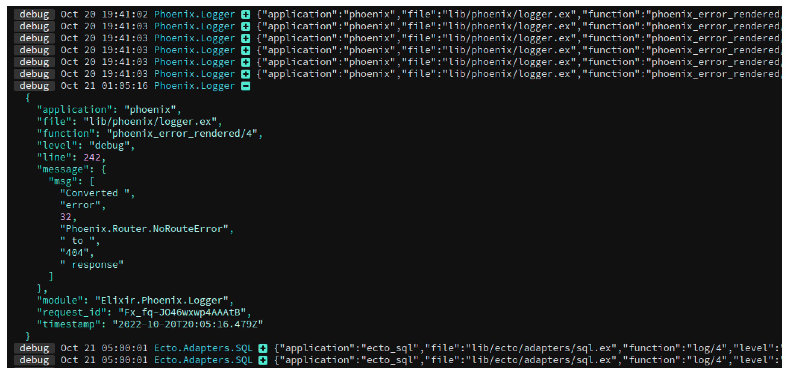
We also gathered real Papertrail log data, which we used for anomaly detection and localization following log parsing. We utilized Papertrail’s search and filtering capabilities to identify the instances or components that may be causing the anomaly. We used the information obtained from the process of anomaly detection and localization to identify and fix the problem’s root cause.
4.3. Results
It is essential to evaluate the performance of a log parser and anomaly-detection system in order to determine how effectively they achieve their objectives. Several different metrics, including parsing accuracy, precision, recall, and F1 score, can be used to evaluate the performance of a log parsing algorithm. Accuracy, the receiver operating characteristic (ROC) curve, and the area under the curve are additional metrics that may be useful for evaluating the performance of a log parsing algorithm (AUC). If the objective was to identify anomalies as precisely as possible, precision may be the most crucial metric to consider. Alternatively, if the objective was to identify as many anomalous instances as possible, recall could be the most important metric. However, we evaluated the log parser based on parsing precision because our current objective is to evaluate the parsing results of the log parser.
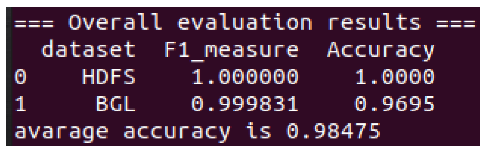
The results of log parsing are depicted in
Figure 3. The results obtained clearly demonstrate the effectiveness of our log parser. It is now time to implement sentence embedding and train the neural network. These results are superior to the logram parser, which achieves an accuracy of 80.9% on HDFS and 58.7% on BGL. It is remarkable that our log parser achieved a parsing accuracy of 98%. This indicates that it can correctly parse the vast majority of log messages, which could be advantageous for extracting useful information and insights from log data.
There are a few factors that contributed to the high parsing accuracy of our log parser:
Robust log parsing algorithm: The log parsing algorithm used by our log parser is robust and able to accurately parse a wide variety of log messages, even if they contain errors or deviations from the expected format.
High-quality training data: The log parser was trained on a large and diverse dataset of log messages, which improved its ability to accurately parse new log messages.
Efficient error handling: The log parser has effective mechanisms for handling and correcting errors in the log messages, which contribute to its high parsing accuracy.
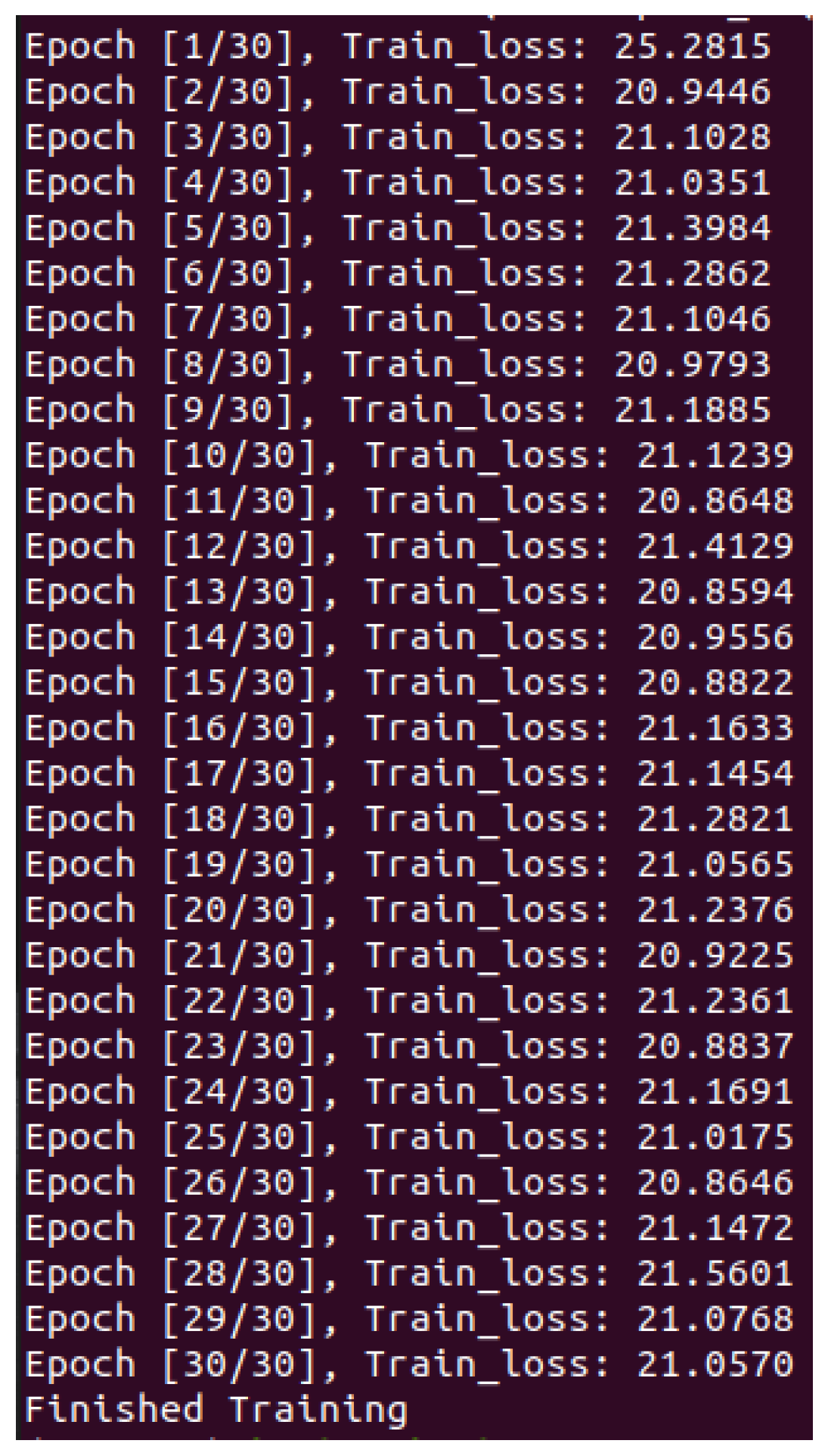
For model training, an attention-based BiLSTM neural network was utilized. In total, 30 epochs were used to train the neural network.
Figure 4 depicts the remarkable results we achieved after training the neural network. Common performance metrics for anomaly-detection systems include detection accuracy, false positive rate, false negative rate, precision, recall, and F1 score. By carefully examining these metrics, the weighted F1 score is the best metric for identifying data anomalies.
Table 3 displays the classification report for the anomaly-detection section.
The classification report is displayed in
Table 3 after the model was updated with the new data. In this research, 88% was the weighted average F1 score attained by the anomaly-detection algorithm. We utilized a weighted average F1 score instead of other commonly used metrics such as precision, recall, and accuracy because there are few samples with anomalous characteristics. The weighted average F1 score accounts for the imbalance between classes in the dataset. In this instance, the F1 score is the average of the F1 scores for each class, with the number of instances in each class serving as the weights.
Anomaly detection is an inherently imbalanced problem, where the number of normal instances significantly outweighs the number of anomalies. In such cases, accuracy can be misleading, as it can be driven by the high accuracy achieved in normal instances while failing to capture the true performance on anomalies. Similarly, precision and recall focus on correctly classifying anomalies, but they may not adequately capture the trade-off between false positives and false negatives, which is crucial in anomaly detection. On the other hand, the F1 score provides a balanced measure that combines precision and recall, making it well suited for imbalanced classification problems. Therefore, in the context of anomaly detection, the weighted average F1 score emerges as a more informative and suitable evaluation metric than accuracy, precision, or recall alone.
We also compared our results with the other methods in the literature.
Table 4 shows the effectiveness of our proposed method.
In the context of anomaly detection and localization, XAI systems can provide explanations for why an anomaly was detected and for its system location. Using XAI for anomaly detection and localization offers a number of advantages:
Improved trust: By providing explanations for their decisions and actions, XAI systems can help to build trust with users and stakeholders who may be skeptical of the capabilities of AI.
Enhanced accountability: XAI systems can help to improve accountability by providing a clear record of the steps that were taken to detect and locate an anomaly, which can be useful for audit and compliance purposes.
Better understandability: XAI systems can help to make the results of anomaly detection and localization more understandable to humans, which can help to improve the effectiveness of the process.
There are several approaches to developing XAI systems for anomaly detection and localization, including:
Rule-based systems: Rule-based systems provide explanations by presenting the specific rules or heuristics that were used to make a decision.
Model-based systems: Model-based systems provide explanations by presenting the underlying model or algorithms that were used to make a decision.
Example-based systems: Example-based systems provide explanations by presenting examples of similar cases that were used to make a decision.
Here, we examine two significant limitations of this study:
First, this study is only capable of identifying anomalies in log data. On the one hand, this study cannot detect abnormalities (such as excessive CPU utilization) revealed by KPI data as opposed to log data. This study employs log time interval change to identify as many potential performance issues as possible, but not all, because not all performance problems are linked to logs.
Second, the scope of this study is limited to log statements whose core meanings are stable despite their constant flux. If the updated logging statement has a different meaning than the previous ones, or if the incoming log message is significantly different from the previous ones, the pre-trained model may not capture the meaning, leading to incorrect results.
4.4. Discussion
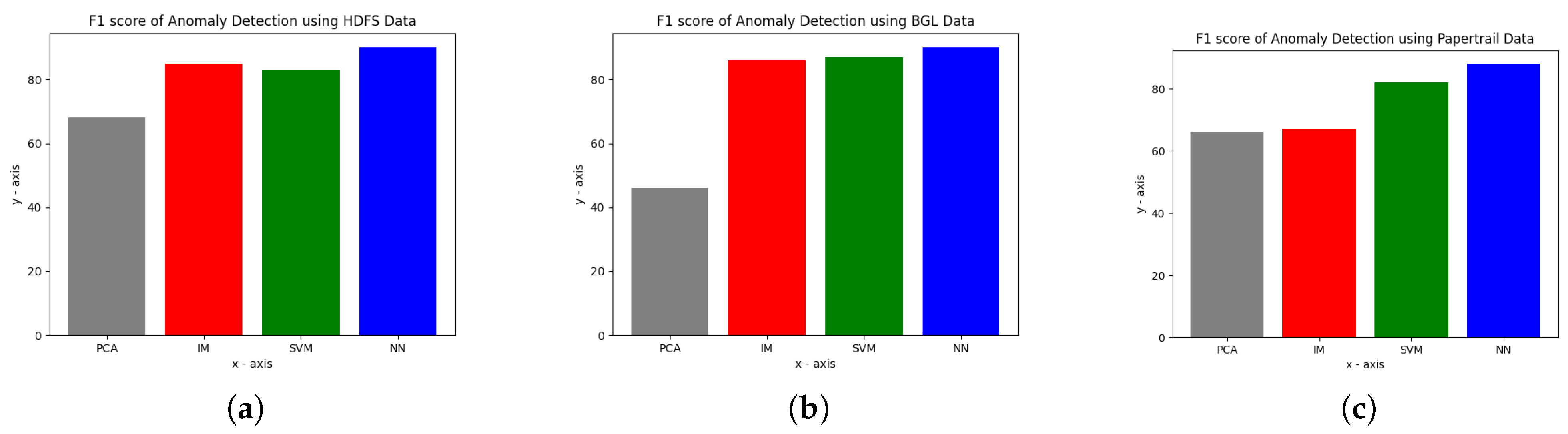
The comparative results of different models are given in
Figure 5. These include deep-learning-based models i.e., Principle Component Analysis (PCA), Initial Margin (IM), Support Vector Machine (SVM), and Neural Network (NN) on HDFS illustrated in
Figure 5a, BGL illustrated in
Figure 5b, and Papertrail illustrated in
Figure 5c data. These illustrated data were actually weighted average F1 scores of different models as we considered them for evaluation purposes.
We also examine the offline training time and online inference time of the anomaly-detection model on the HDFS dataset. This investigation’s execution time is measured in milliseconds per sequence (ms/seq).
In
Table 5, we compare the runtime of the anomaly-detection component of deep-learning-based models and models that do not use deep learning. Training time corresponds to offline training cost, while real or inference time corresponds to online detection time. These times were carried out by using a Python library “timeit”, which is used to calculate the execution time of the algorithm. Due to the fact that a deep-learning-based model must be trained over multiple epochs, only the runtime of one epoch is presented here. Due to the immense complexity of deep-learning-based models and the limited resources of this research’s experimental contexts, it is evident that deep-learning-based models are significantly slower than models that do not utilize deep learning. The ADAL-NN requires four times as much training as alternatives. This is acceptable, as the overhead incurred during offline training has no bearing on the online runtime of anomaly detection. The online inference time of the ADAL-NN is roughly double that of LogRobust. Given that this model is a three-classification problem and LogRobust is a two-classification task, it may take longer to learn and predict an additional class.
A large-scale system may generate over 60 GB of logs per hour, or 120 million log lines [
2] (i.e., 6 million log sequences assuming each sequence comprises 20 log lines). According to
Table 3, due to the limited processing power and device memory of a single Z-book system, it takes approximately one thousand minutes. We have also run the ADAL-NN in parallel on an eight-core CPU, which has a significant impact on the online detection time. The results indicate that it takes approximately 50 min to process such a large volume of log data.
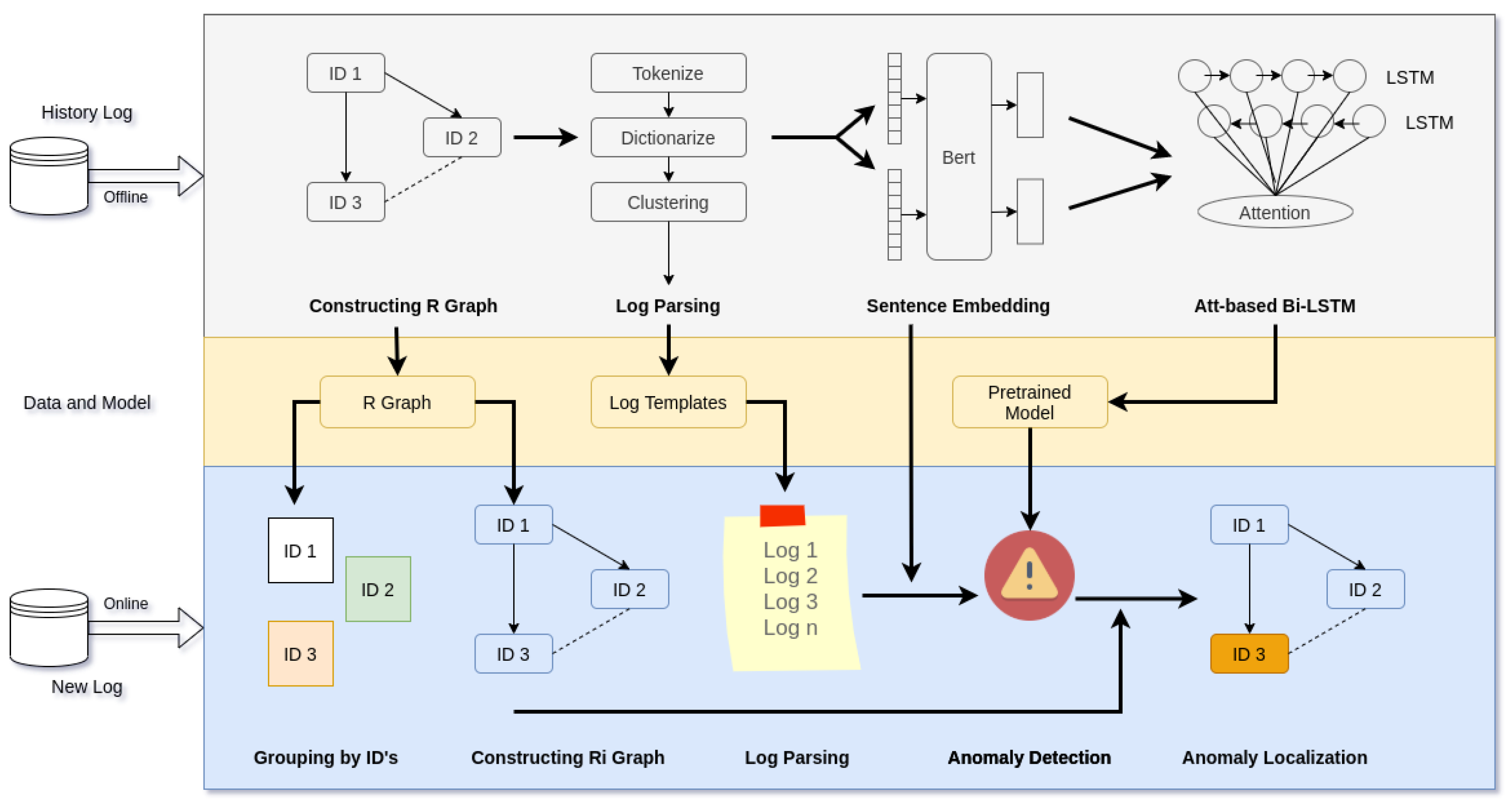
The proposed method presents a notable advancement in terms of efficiency, robustness, and generalization compared to existing approaches. Firstly, in terms of efficiency, the method incorporates various optimizations and techniques that enable faster processing and analysis of log data. By constructing the ID relation graph during the offline phase and leveraging log parsing and sentence embedding techniques, the method efficiently extracts and encodes the relevant semantic and temporal information from log sequences. This streamlined process reduces computational overhead and improves the overall efficiency of anomaly detection and localization.
Secondly, the method exhibits enhanced robustness compared to previous approaches. By employing an attention-based Bi-LSTM, the model effectively captures the intricate patterns and dependencies within log sequences, enabling accurate detection and localization of anomalies. The use of deep learning techniques enhances the model’s ability to handle complex and diverse log data, making it more robust in detecting anomalies across different scenarios and system environments. Additionally, the method’s integration of anomaly identification and localization components further strengthens its robustness by providing a comprehensive understanding of the detected anomalies.
Lastly, the proposed method demonstrates superior generalization capabilities. Through the utilization of large-scale datasets such as HDFS, BGL, and Custom, the model is trained on diverse log data, enabling it to learn and generalize patterns across different domains and applications. This generalization capability allows the method to effectively adapt to new and unseen log data, making it highly applicable in real-world scenarios where log data patterns may vary. The incorporation of explainable AI techniques further enhances the model’s generalization by providing transparent and interpretable explanations for anomaly detection and localization, ensuring its applicability across various domains and facilitating decision-making processes.
In summary, the proposed method offers significant advancements in terms of efficiency, robustness, and generalization. By leveraging optimized techniques, deep learning models, and explainable AI components, the method achieves faster processing, accurate anomaly detection, comprehensive localization, and adaptability to diverse log data, making it a highly promising approach in the field of anomaly detection and localization.
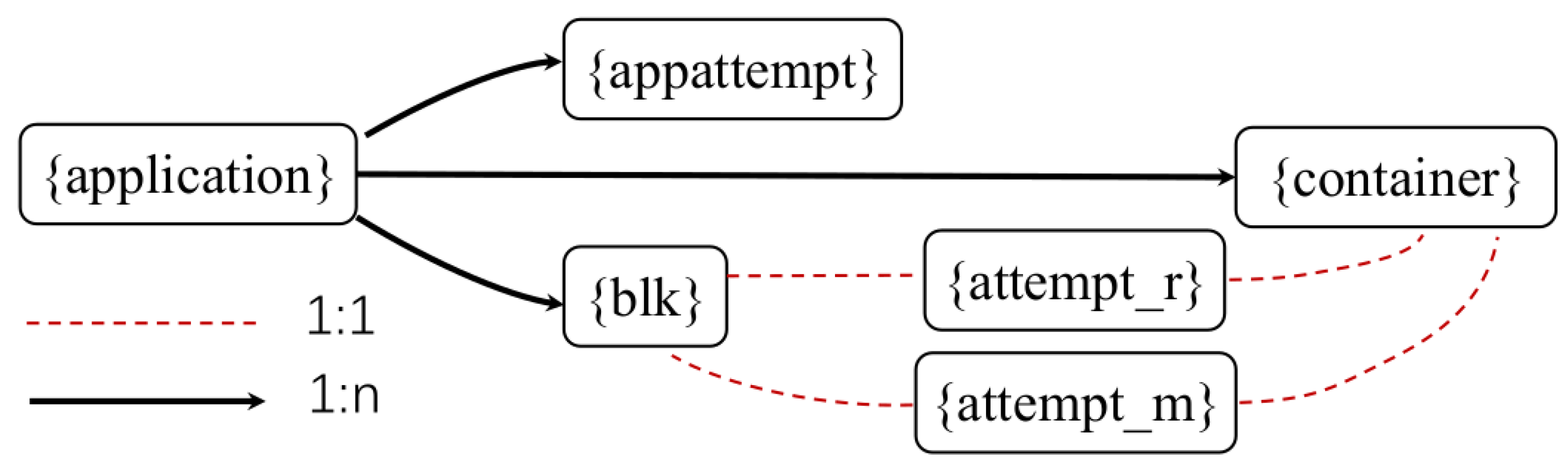
This research provides a case study of a real-world system, Hadoop, to further illustrate the identification and localization of anomalies. The
R graph of a Hadoop cluster is illustrated in
Figure 6. Hadoop consists of six distinct types. The relationship between types is represented by arrow lines, with the 1:1 relationship indicated by a red dashed line and the 1:n relationship indicated by a black line. For instance, if an application creates multiple blocks, their relationship is 1:n. In our research, the 1:1 correlation is eliminated.
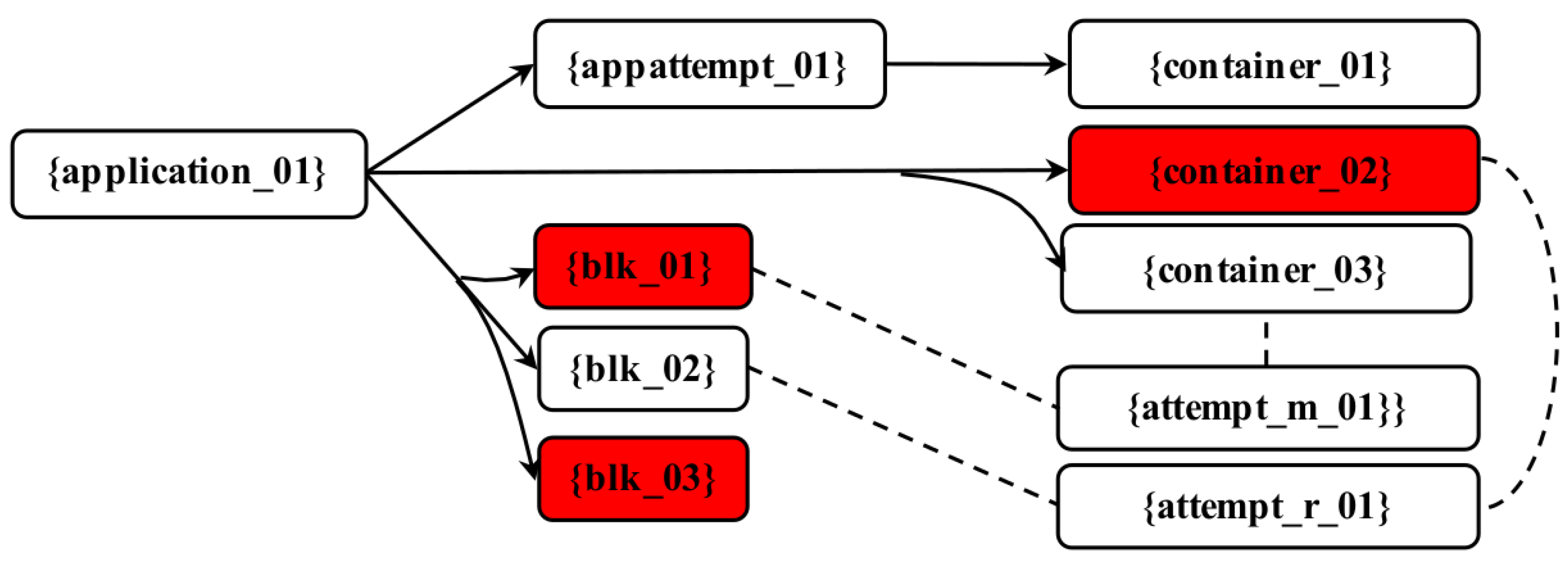
Following that, we provide a real-world anomalous instance. To begin, a series of incoming logs progressively launches the
R graph as the
graph. In reality, application 01 generates a total of 14 blocks and 16 containers. In
Figure 7, we only display the simplified
graph with three blocks, three containers, one app attempt, one attempt r, and one attempt m due to space constraints.
This research first identifies anomalies in log data organized by block ID and labels blk 01 as an anomalous block. Following that, an exception is detected in block 03; consequently, the ADAL-NN identifies block 03 as aberrant as well. Ultimately, the ADAL-NN method detects a killing signal in container 02, which is labeled as flawed. In
Figure 7, all of the incorrect instances in A are colored red. The graph
is then subjected to heuristic searching. The ADAL-NN reports the anomalous instances blk 01, blk 03, and container 02 because they are leaf nodes in the
graph. Consequently, we can identify anomalies in Hadoop at the instance level (blk and container in this example). Such information can greatly aid developers in identifying the source of the issue. We can see, for instance, that not all blocks and containers are affected by these anomalies. In slave clusters, we can assume that a node failure is possible. The associated logs of blk 01, blk 03, and container 02 indicate that slave 2 is experiencing a network issue. Therefore, when we encounter anomalies, this research can aid us in swiftly identifying and analyzing root causes.
4.5. Comparison with Deep Learning Models
To further demonstrate the effectiveness of our proposed method, we conducted additional experiments comparing it with state-of-the-art deep learning models commonly used for anomaly detection. By including these comparisons, we aim to showcase the superiority of our approach over both traditional and modern anomaly-detection techniques.
We selected the three widely used deep learning models in the task of anomaly detection, which are Autoencoders (AE), Variational Autoencoders (VAE), and Recurrent Neural Networks (RNN). These models were chosen based on their popularity and proven performance in anomaly-detection tasks. For each deep learning model, we implemented the necessary architecture and trained it using the same dataset and evaluation metrics as our proposed method. We ensured that the hyperparameters and training settings were appropriately tuned for each model. We then compared the performance of our proposed method with these deep learning models using the F1 score metrics.
In the HDFS anomaly-detection evaluation, the F1 scores for the NN, AE, VAE, and RNN models were 0.90, 0.87, 0.88, and 0.88, respectively. Similarly, in the BGL anomaly-detection evaluation, the F1 scores for the NN, AE, VAE, and RNN models were 0.90, 0.89, 0.90, and 0.89, respectively. Furthermore, in the PT anomaly-detection evaluation, the F1 scores for the NN, AE, VAE, and RNN models were 0.88, 0.86, 0.87, and 0.87, respectively. For better demonstration, we added these results into
Table 6. These scores highlight the capability of the models to identify anomalies in the HDFS, BGL, and PT datasets.
The results were obtained through rigorous cross-validation and statistical analysis to ensure reliable comparisons. By including comparisons with deep learning models, we demonstrate the effectiveness and superiority of our proposed method in detecting and localizing anomalies in unstructured logs.
4.6. Future Work
Future research and development in the field of anomaly detection and localization could be conducted in the following areas.
Researchers can continue to improve the accuracy and robustness of existing anomaly-detection algorithms by developing more effective feature extraction techniques, incorporating additional context and background knowledge, and addressing class imbalance issues.
Developing new approaches for anomaly detection: There is a need for the development of new anomaly-detection methods that can handle a variety of data types, such as high-dimensional data or streaming data, and that can be applied to a wide variety of use cases.
Including domain-specific expertise: Anomalies are frequently easier to detect and localize when domain-specific knowledge is considered. For instance, in a manufacturing environment, understanding the normal operation of a specific machine can help to more precisely identify and locate anomalies.
Exploiting temporal dependencies: numerous anomalies exhibit temporal dependencies, which means they tend to occur in a particular pattern over time. The accuracy and effectiveness of anomaly-detection algorithms can be improved by incorporating this information.
Creating robust and effective localization techniques: Anomaly localization is frequently a difficult task, especially when the data are of high dimension or when the anomalies are small or subtle. The development of robust and efficient localization methods that can precisely identify the location and extent of anomalies can be a significant area of future research.
In many applications, the characteristics of the data and the types of anomalies that can occur can change over time. Important research topics include the development of anomaly-detection algorithms that can adapt to these changes and continue to detect and localize anomalies effectively.


