A Microscopic Traffic Model Considering Driver Reaction and Sensitivity

Abstract

A new microscopic traffic model is proposed that characterizes driver response according to reaction and sensitivity. Driver response in the intelligent driver (ID) model is based on a fixed acceleration exponent and so does not follow traffic physics. This inadequate characterization results in unrealistic traffic behavior. With the proposed model, drivers can be aggressive, sluggish, or typical. It is shown to be string stable, and for appropriate distance headway and velocity (speed), the traffic flow is smooth. Furthermore, the proposed model has better stability than the ID model because it is based on driver reaction and sensitivity, while the ID model is based on a fixed exponent. The ID and proposed models are evaluated on a circular road of length 1200 m with a platoon of 21 vehicles for 150 s. The results obtained show that the proposed model characterizes traffic more realistically than the ID model.

1. Introduction

Traffic models are important for vehicle flow characterization [1]. They are used to develop traffic forecasting and control strategies and improve road infrastructure utilization to mitigate congestion [2,3,4]. During congestion, stop and go waves cause drivers to vary their speed, which creates poor traffic dynamics [5,6]. The distances between vehicles and the time required to adjust (align) to conditions ahead affect driver response and can result in significant variations in traffic flow [7]. Time headway, $\tau$, is the time required to adjust to traffic conditions ahead, and the distance headway is traversed during $\tau$ [8]. A driver responds slowly with a large distance headway and quickly with a small distance headway [9]. Furthermore, driver response is affected by sensitivity, which is proportional to the change in velocity [9]. Since driver response is not the same for all traffic conditions, it should be considered in a model for accurate and realistic traffic characterization.

Three categories of models have been used for traffic flow: microscopic, macroscopic, and mesoscopic. Microscopic models are used to study individual vehicle behavior and employ parameters such as velocity, position, time, and distance headway. They are often based on driver physiological and psychological responses [10] and are employed to predict vehicle dynamics [11,12,13]. Macroscopic models are used to study aggregate traffic behavior. Mesoscopic models blend microscopic and macroscopic models and typically involve probability distributions [14].

Gazis et al. [15] introduced a microscopic model that considers how drivers respond to forward vehicles using velocity differences. However, this model neglects changes in driver behavior due to traffic conditions. Drivers adjust their speed to forward vehicles with a constant delay of $1.30$ s, which can result in poor traffic behavior. Newell [16] developed a microscopic model that characterizes traffic flow during congestion. In this model, velocity is dependent on the distance headway. A larger distance headway reduces congestion so the velocity increases. However, a larger change in velocity results in excessive acceleration, which is not realistic [17]. Bando et al. [18] proposed an improvement to the Newell model, but it ignores velocity differences, which can lead to instability. The equilibrium velocity distribution is density-dependent so the velocity decreases with increasing density. However, deviations from this distribution lead to uniform acceleration, which is unrealistic. Furthermore, driver behavior is the same for all conditions, which does not follow traffic physics.

Bosch [19] developed a model using regression, but it has many parameters so the complexity is high. Helbing and Tilch [20] proposed a model that employs velocity differences to characterize velocity and time headway during congestion, but acceleration can be unrealistic. Gipps [21] created a model that considers acceleration and driver behavior, but the accuracy is limited to a narrow set of parameters.

Treiber, Henneck, and Helbing [17] developed the Intelligent Driver (ID) model, which incorporates driver reaction and takes into account the velocity and distance headway of preceding vehicles [22,23,24]. A limitation of this model is that it employs a fixed acceleration exponent so driver behavior is not considered. This can produce unrealistic results. The ID model was modified in [25] to incorporate driver intent by considering deceleration at intersections. The safe distance between vehicles with the ID model is small at high velocities, which can result in accidents when employed in applications such as Adaptive Cruise Control (ACC). This distance has been adjusted using velocity-based parameters [26]. The ID model has been used to characterize the car-following behavior and stability of Connected and Autonomous Vehicles (CAVs) [27,28]. However, it fails to capture the characteristics of CAVs in real traffic environments [29].

Advanced Driver Assistant Systems (ADASs) are deployed in many new vehicles [30] and interest in automated driving (AD) is increasing [31]. Traffic safety and environmental impact can be examined using microscopic models, but the connection to real traffic is unclear [30]. However, they have been used in the Project for the Establishment of Generally Accepted quality criteria, tools and methods as well as Scenarios and Situations (PEGASUS) to address AD challenges [31].

Software such as SUMO, PTV Vissim, and CARLA has been developed to predict traffic behavior. SUMO is a multi-modal microscopic traffic simulator that can be used to model large traffic networks such as in cities [32]. It has been integrated with the ID model to examine features such as free and congested flow, but driver behavior is not considered [33]. SUMO can be used to investigate multi-lane streets with lane changing, intersections with streets having the same or different priorities such as right-before-left, and lane-to-lane connections [32].

Connected vehicles interact with their surroundings to ensure safety [34]. PTV Vissim [35] can be used to forecast freeway capacity and facilitate CAV deployment [36]. However, characterizing the interactions between autonomous and non-autonomous vehicles poses significant challenges [37]. The NGSIM dataset [38] is widely used in transportation research. However, it only focuses on human-driven vehicle behavior and traffic flow. Automated Driving System (ADS) data were introduced in [39] for CAV analysis such as the interaction between human-driven and ADS-equipped vehicles, car-following behavior, and traffic flow. CARLA is an open-source urban driving simulator designed to facilitate the development and validation of autonomous vehicles under different weather and lighting conditions [40].

A microscopic traffic model is proposed that models the acceleration exponent in the ID model [17] using driver reaction and sensitivity. Driver sensitivity is the reaction to changes in velocity and can be typical, sluggish, or aggressive. This variable exponent provides better stability and is more realistic than the fixed exponent in the ID model. This is because it is based on real traffic parameters. The performance of the proposed and ID models is evaluated on a single-lane circular road of length $1200$ m. A circular road can be considered worst-case because there is no loss of vehicles. A platoon of $21$ vehicles is considered for $150$ s. The results obtained show that the changes in density with the proposed model are appropriate and the velocity and density evolve smoothly over time.

2. Traffic Models

The ID model characterizes vehicle movement and is given by [17]

$$\frac{dv}{dt}=a\left(1-{\left(\frac{v}{v_{max}}\right)}^{\delta }-{\left(\frac{D}{s}\right)}^2\right),$$

(1)

where $a$ is the maximum acceleration, v is the average velocity, $v_{max}$ is the maximum velocity (speed limit) on the road, s is the actual distance headway between vehicles, $s_j$ is the jam distance as shown in Figure 1, which is the smallest possible distance between vehicles at maximum density, $\tau$ is the time headway during alignment when a change in velocity $\Delta v$ occurs, and $\delta$ is the acceleration exponent. This exponent is a constant chosen to fit traffic behavior and is not based on traffic dynamics. According to $\left(1\right)$, acceleration is a function of driver response, the distance between vehicles, and the time needed to adapt to traffic conditions. Driver response is affected by the ratio of average velocity to maximum velocity. For a smooth flow with little acceleration, this ratio approaches $1$ so the velocity is near maximum. The term $D$ represents the desired distance headway during traffic alignment and can be expressed as [17]

$$D=s_j+\tau v+\frac{v\Delta v}{2\sqrt{ab}},$$

(2)

where $b$ is the minimum acceleration. The ID model parameters are given in Table 1. In this model, driver response to changes in traffic conditions is described by the fixed exponent $\delta$, so vehicle behavior is the same for all scenarios, which is unrealistic. Therefore, a model is proposed that characterizes driver response using a variable exponent that is based on traffic physics.

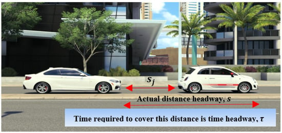
Figure 1. The distance and time headways.

Table 1. ID model parameters.

Parameter	Description
$dv/dt$	Driver response
$a$	Maximum acceleration
$v$	Average velocity
$v_{max}$	Maximum velocity
$s$	Actual distance headway
$s_j$	Jam spacing
$\tau$	Time headway
$b$	Minimum acceleration
$\Delta v$	Change in velocity during traffic alignment
$\delta$	Acceleration exponent (constant)

A driver reacts based on the acceleration required to align to forward vehicles. This acceleration depends on the time headway between vehicles so a large time headway results in a slow reaction. Conversely, driver reaction is quick for a small time headway and the acceleration is large. Thus, driver reaction during alignment can be characterized as

$$V_t=a\tau ,$$

(3)

However, the ratio of actual distance headway $s$ to desired distance headway $D$ influences this reaction, so (3) is modified to

$$V_r=a\tau \left(\frac{s}{D}\right).$$

(4)

The value of $\frac{s}{D}$ varies between $0$ and $1$. When $\frac{s}{D}=0$, driver response is 0 so there is no change in velocity. In this case, the density is maximum, i.e., during congestion when there is no vehicle movement. When $\frac{s}{D}=1$, the change in velocity is large so the traffic flow is smooth and the maximum speed is achieved.

Driver sensitivity plays a significant role in the driver response. The safe time headway is defined as

$${\tau }_s={\tau }_p+{\tau }_r+\tau ,$$

(5)

where ${\tau }_p$ is the time required to perceive changes in traffic, ${\tau }_r$ is the time required to react, and $\tau$ is the time required to cover the distance headway. The safe time headway is required to cover the distance headway safely and avoid accidents. Driver response is fast when the time headway is smaller than the safe time headway. In heterogeneous traffic, vehicles frequently change lanes to occupy any forward distance so vehicles align quickly to avoid lane changes by other vehicles. This reduces the distance headway and increases the time headway, and is a major cause of stop and go traffic. When the time headway is greater than the safe time headway, traffic flow is smooth and the distance headway can increase. In this case, lane changes do not reduce the time headway and driver response is slow.

Driver sensitivity can be expressed as $\frac{\tau }{{\tau }_s}$. A driver is aggressive when $\frac{\tau }{{\tau }_s}<1$ and sluggish when $\frac{\tau }{{\tau }_s}>1$. For a typical driver, $\frac{\tau }{{\tau }_s}=1$. Therefore, the driver response from (4) can be expressed as

$$a\tau \left(\frac{s}{D}\right)\left(\frac{\tau }{{\tau }_s}\right).$$

(6)

The proposed model is obtained by replacing $\delta$ in (1) with (6) giving

$$\frac{dv}{dt}=a\left(1-{\left(\frac{v}{v_{max}}\right)}^{a\tau \left(\frac{s}{D}\right)\left(\frac{\tau }{{\tau }_s}\right)}-{\left(\frac{D}{s}\right)}^2\right).$$

(7)

With this model, changes in velocity are affected by the time and distance headway. It can be extended to include lane changes by considering lateral distances [41]. Predicting turns and stops at intersections is required for ADASs. This can be achieved with the proposed model for both car following and turning at intersections by inferring driver response [25]. It can also be incorporated into ACC and cooperative ACC systems [42].

The traffic density is given by $\rho =\frac{1}{s_e}$ [5] where $s_e$ is the equilibrium distance headway. At equilibrium, changes in velocity are negligible, that is, $\Delta v=0$. Incorporating this equilibrium condition in (2) and substituting (1) gives $s_e$ for the ID model [17] as

$$s_e=(s_j+\tau v){\left(1-{\left(\frac{v}{v_{max}}\right)}^{\delta }\right)}^{-\frac{1}{2}}.$$

(8)

For the proposed model, substituting $\delta$ with (6) in (8) gives

$$s_e=(s_j+\tau v){\left(1-{\left(\frac{v}{v_{max}}\right)}^{a\tau \left(\frac{s}{D}\right)\left(\frac{\tau }{{\tau }_s}\right)}\right)}^{-\frac{1}{2}}.$$

(9)

According to (8), the equilibrium distance headway between vehicles with the ID model is the same for all traffic conditions because $\delta$ is a constant chosen as a compromise to fit all scenarios. Conversely, (9) is based on the distance and time headways and so is not a constant. Thus, changes in equilibrium distance headway are affected by driver sensitivity and reaction.

The traffic flow is the product of velocity and density $Q=\frac{v}{s_e}$ [22] so the ID model flow is

$$Q=\frac{1}{(s_j+\tau v){\left(1-{\left(\frac{v}{v_{max}}\right)}^{\delta }\right)}^{-\frac{1}{2} }}v,$$

(10)

while the proposed model flow is

$$Q=\frac{1}{(s_j+\tau v){\left(1-{\left(\frac{v}{v_{max}}\right)}^{a\tau \left(\frac{s}{D}\right)\left(\frac{\tau }{{\tau }_s}\right)}\right)}^{-\frac{1}{2} }}v,$$

(11)

This indicates that the traffic flow with the proposed model is based on driver reaction and sensitivity. A smaller distance headway results in a faster driver response as there are significant interactions between vehicles, i.e., during congestion [9], so the flow is low. Conversely, with a large distance headway, driver response is slow and there are few interactions between vehicles so the flow is high [9]. Furthermore, a higher sensitivity results in larger changes in traffic flow.

Obtaining real speed (velocity) and headway data can be expensive and challenging. These data are prone to noise and inaccuracies that must be considered when calibrating a model. Traffic model calibration is employed to determine appropriate parameter values [43]. One method to address the problems with sensor noise is sensor fusion, which utilizes both Global Navigation Satellite System (GNSS) and Inertial Measurement Unit (IMU) information [44]. The GNSS provides global position information, while the IMU measures acceleration and angular rates. Techniques such as filtering, weighting, redundancy, and error modeling can also be employed to reduce the effects of noise. The calibration process is often iterative to refine the parameters and achieve more accurate traffic modeling [43,44].

3. Stability Analysis

In this section, the theoretical and numerical stability of the ID and proposed models are evaluated.

3.1. Theoretical Stability

The stability of both the ID and proposed models is analyzed over an infinite road. The driver response and vehicles are assumed identical and the equilibrium distance headway $s_e$ is maintained between all vehicles [45]. Thus, drivers align to forward conditions with little acceleration, and only small changes in equilibrium velocity $v_e\left(s_e\right)$ occur. The changes in distance headway $x$ are therefore small as are the changes in velocity $y$. The distance headway during a change in velocity is then

$$s=s_e+x,$$

(12)

and the corresponding velocity is

$$v=v_e\left(s_e\right)+y.$$

(13)

During traffic alignment over the distance headway, the temporal change in velocity [37] is

$$x\left(t\right)=\frac{dx}{dt}=y_l-y_F,$$

(14)

where the subscripts $l$ and $F$ denote the leading and following vehicles, respectively. The changes in headway are small as the changes in $v_e\left(s_e\right)$ are small, so $y\left(t\right)$ during alignment can be expressed as [45]

$$y\left(t\right)=\frac{dy}{dt}=f_s{x}_F+(f_v+f_{\Delta v})y_F-f_{\Delta v}{y}_l,$$

(15)

where $f_{\Delta v}$ is the partial derivative with respect to the change in velocity, $f_v$ is the partial derivative with respect to velocity, and $f_s$ is the partial derivative with respect to distance headway, and are given by

$$f_s=\frac{\partial f}{\partial s}, f_v=\frac{\partial f}{\partial v}, \mathrm{and} f_{\Delta v}=\frac{\partial f}{{\partial }_{\Delta v}}.$$

Equations (14) and (15) are solved using Fourier-Ansatz as

$$y\left(t\right)=\widehat{y}{e}^{\gamma t+ik},$$

(16)

$$u\left(t\right)=\widehat{u}{e}^{\gamma t+ik},$$

(17)

so (16) and (17) take the form

$$\left(\begin{array}{c}x\left(t\right)\\ y\left(t\right)\end{array}\right)=\left(\begin{array}{c}\widehat{x}\\ \widehat{y}\end{array}\right)e^{\gamma t+ik},$$

(18)

where $\gamma =\alpha +i\omega$ is the change in traffic oscillations during alignment and $i=\sqrt{-1}$. The real part $\alpha$ denotes the change in amplitude, $\omega =\frac{2\pi }{T}$ is the oscillation frequency, $T$ is the oscillation period, $k$ is the phase shift that corresponds to the delay experienced by a driver [45], and $\widehat{y}$ and $\widehat{x}$ are the changes in velocity and distance headway, respectively.

Substituting (18) in (14) and (15) gives

$$x\left(t\right)=y-y{e}^{ik},$$

(19)

$$y\left(t\right)=f_{s}x{e}^{ik}+\left(f_v+f_{\Delta v}\right)y{e}^{ik}-f_{\Delta v}y.$$

(20)

The model is stable if the real parts of the eigenvalues are negative. The eigenvalues are obtained from

$$\left|J-\left(\begin{array}{cc}\lambda & 0\\ 0& \lambda \end{array}\right)\right|=0,$$

(21)

where $J$ is the Jacobian matrix given by

$$J=\left(\begin{array}{cc}{j}_{11}& j_{12}\\ j_{21}& j_{22}\end{array}\right),$$

and $j_{11}$ and $j_{21}$ are the partial differentials of (19) and (20) w.r.t. $x$ and $j_{12}$ and $j_{22}$ are the partial differentials of (19) and (20) w.r.t $y$ so that

$$J=e^{ik}\left(\begin{array}{cc}0& e^{-ik}-1\\ f_s& \left(f_v+f_{\Delta v}\right)-f_{\Delta v}{e}^{-ik}\end{array}\right).$$

(22)

Then substituting (22) in (21) we have

$$\left|\begin{array}{cc}\lambda & 1-e^{-ik}\\ -f_s& \lambda -f_v-f_{\Delta v}+f_{\Delta v}{e}^{-ik}\end{array}\right|=0,$$

(23)

which gives

$${\lambda }^2+\left(-f_v-f_{\Delta v}+f_{\Delta v}{e}^{-ik}\right)\lambda +f_s\left(1-e^{-ik}\right)=0$$

(24)

Let $X\left(k\right)=-f_v-f_{\Delta v}+f_{\Delta v}{e}^{-ik}$ and $Y\left(k\right)=f_s\left(1-e^{-ik}\right)$ in (24) so that

$${\lambda }^2+X\left(k\right)\lambda +Y\left(k\right)=0$$

(25)

The eigenvalues from $\left(25\right)$ are

$${\lambda }_{1,2}=-\frac{X\left(k\right)}{2}\left( 1\pm \sqrt{1-\frac{4Y\left(k\right)}{X^2\left(k\right)}}\right),$$

(26)

The model is string stable [45] if the real parts of the eigenvalues are negative. In this case, vehicles maintain the distance headway and changes in the equilibrium velocity are small [46]. Then the oscillations in flow decay over time so it is stable (smooth). A model is unstable if the flow increases over time. An example is stop and go traffic, which occurs during congestion. In this case, acceleration is high, whereas in string stable traffic, acceleration is low [5]. In unstable traffic, $k\to 0$ so there is a negligible delay between changes in flow (traffic waves) [45]. Using Taylor series, $Y\left(k\right) \mathrm{and} X\left(k\right)$ can be approximated for a small delay, i.e., $k\to 0$, as

$$X\left(k\right)=-f_v-i{f}_{\Delta v}k,$$

(27)

$$Y\left(k\right)=i{f}_{s}k+\frac{f_s}{2}{k}^2.$$

(28)

At equilibrium [45]

$$f_s=-v_e^{\prime }\left(s_e\right)f_v.$$

(29)

where $v_e^{\prime }\left(s_e\right)$ is the gradient of the equilibrium velocity (speed) with respect to the equilibrium distance headway. Substituting (29) in (28) gives

$$Y\left(k\right)=-i{v}_e^{\prime }\left(s_e\right)f_v-\frac{v_e^{\prime }\left(s_e\right)}{2}{f}_v.$$

(30)

Let

$$\begin{gathered} X\left(k\right)=a_1+a_{2}k, \\ Y\left(k\right)=b_{1}k+b_2{k}^2, \end{gathered}$$

(31)

where

$$\begin{gathered} a_1=-f_v, \\ {a}_2=-i{f}_{\Delta v}, \\ {b}_1=-i{v}_e^{\prime }\left(s_e\right)f_v=i{v}_e^{\prime }\left(s_e\right)a_0, \\ {b}_2=-\frac{v_e^{\prime }\left(s_e\right)}{2}{f}_v=\frac{v_e^{\prime }\left(s_e\right)}{2}{a}_0. \end{gathered}$$

(32)

Employing a Taylor series approximation, the square root in (26) becomes

$$\sqrt{1-\frac{4Y\left(k\right)}{X^2\left(k\right)}}=1-\frac{2Y\left(k\right)}{X^2\left(k\right)}-\frac{2Y^2\left(k\right)}{X^4\left(k\right)}.$$

(33)

which results in

$${\lambda }_2=\frac{-Y\left(k\right)X^2\left(k\right)-Y^2\left(k\right)}{X^3\left(k\right)}.$$

(34)

and from (31)

$${\lambda }_2=-\frac{b_1}{a_1}k+\left(\frac{b_1{a}_2}{a_1^2}-\frac{b_2}{a_1}-\frac{b_1^2}{a_1^3}\right)k^2.$$

(35)

Now using (32) we obtain

$${\lambda }_2=-i{v}_e^{\prime }\left(s_e\right)k+\frac{v_e^{\prime }\left(s_e\right)}{f_v}\left[\frac{-2f_{\Delta v}-f_v}{2}-v_e^{\prime }\left(s_e\right)\right]k^2.$$

(36)

The real part of (36) denotes the change in amplitude of the traffic oscillations (growth rate). The traffic flow is string stable if this is negative. Since

$$v_e^{\prime }\left(s_e\right) \ge 0 \mathrm{and} f_v<0,$$

(37)

$\left[\frac{-2f_{\Delta v}-f_v}{2}-v_e^{\prime }\left(s_e\right)\right]$ is the string stability criterion [26], i.e.

$$v_e^{\prime }\left(s_e\right)\le -\frac{f_v}{2}-f_{\Delta v}.$$

(38)

From (37) and (38), the product of $\left[-\frac{2f_{\Delta v}-f_v}{2}-v_e^{\prime }\left(s_e\right)\right]$ and $\frac{v_e^{\prime }\left(s_e\right)}{f_v}$ indicates that ${\lambda }_2$ has a negative real part.

At equilibrium, $f_v$ and $f_{\Delta v}$ for the ID model (1) are

$$f_v=a\left(-\frac{\delta v_e{\left(s_e\right)}^{\delta -1}}{v_{max}^{\delta }}-\frac{2\tau \left(s_j+v_e\left(s_e\right)\tau \right)}{s_e^2}\right),$$

(39)

$$f_{\Delta v}=-\frac{v_e\left(s_e\right)}{s_e}\sqrt{\frac{a}{b}}\left(\frac{s_j+v_e\left(s_e\right)\tau }{s_e}\right).$$

(40)

Using (39) and (40), the string stability criterion from (38) is

$$v_e^{\prime }\left(s_e\right)\le \frac{a\left(\delta {\left(s_e\right)}^2{v}_e{\left(s_e\right)}^{\delta -1}+2\tau s_j{v}_{max}^{\delta }+2v_e\left(s_e\right){\tau }^2{v}_{max}^{\delta }\right)}{2{\left(s_e\right)}^2{v}_{max}^{\delta }}+\frac{v_e\left(s_e\right)\sqrt{ab}\left(s_e+\tau v_e\left(s_e\right)\right)}{{\left(s_e\right)}^{2}b}$$

(41)

This shows that changes in velocity with the ID model are characterized by the constant $\delta$. A traffic string is more stable with a larger value of $\delta$, but in this case, congestion ends quickly. Thus, making $\delta$ larger to ensure stability ignores traffic physics and results in unrealistic traffic behavior [11]. The velocity changes during traffic alignment are affected by driver sensitivity and reaction. Thus, to ensure appropriate behavior, $\delta$ in (41) is replaced with (6), which gives the proposed model stability criteria as

$$\begin{gathered} v_e^{\prime }\left(s_e\right)\le \frac{a\left(a\tau \left(\frac{s}{D}\right)\left(\frac{\tau }{{\tau }_s}\right){\left(s_e\right)}^2{v}_e{\left(s_e\right)}^{a\tau \left(\frac{s}{D}\right)\left(\frac{\tau }{{\tau }_s}\right)-1}+2\tau s_j{v}_{max}^{a\tau \left(\frac{s}{D}\right)\left(\frac{\tau }{{\tau }_s}\right)}+2v_e\left(s_e\right){\tau }^2{v}_{max}^{a\tau \left(\frac{s}{D}\right)\left(\frac{\tau }{{\tau }_s}\right)}\right)}{2{\left(s_e\right)}^2{v}_{max}^{a\tau \left(\frac{s}{D}\right)\left(\frac{\tau }{{\tau }_s}\right)}}+ \\ \frac{v_e\left(s_e\right)\sqrt{ab}\left(s_e+\tau v_e\left(s_e\right)\right)}{{\left(s_e\right)}^{2}b}. \end{gathered}$$

(42)

Thus, with the proposed model, changes in velocity are based on driver sensitivity and reaction. Drivers are more sensitive to large changes in velocity, which results in a traffic flow that is string stable [9]. Furthermore, a smaller distance headway than at equilibrium means vehicles move slowly so congestion takes longer to dissipate [2]. Conversely, a larger distance headway than at equilibrium means congestion dissipates quickly resulting in a stable traffic flow [11].

3.2. Numerical Stability

Both models are evaluated over a $1000$ m single-lane circular road for $180$ s with a platoon of $21$ vehicles. The time headway with the ID model is $2$ s. For the proposed model, $\tau =1$ s, which corresponds to an aggressive driver, $\tau =2.5$ s, which corresponds to a sluggish driver, and $\tau =2$ s, which corresponds to a typical driver, are considered. The value of $h=\frac{s}{D}$ ranges between $0$ and $1$, so here $0.3, 0.5,$ and $1$ are used. The value of $\delta$ varies between $1$ and $\infty$, and is usually $4$ [17]. Hence, the values of $\delta$ considered are $1, 4,$ and $20$. The initial equilibrium velocity is $4$ m/s and the number of vehicles is $21$. A perturbation is induced at $30$ s based on the minimum acceleration. The stability analysis parameters for the ID and proposed models are given in Table 2.

Table 2. Parameters for stability analysis.

Parameter	Value
Proposed model acceleration, $a$	$1.5$ m/s2
Time headway for the ID model, $\tau$	$2$ s
Time headway for the aggressive driver, τ	$1$ s
Time headway for the sluggish driver, $\tau$	$2.5$ s
Time headway for the typical driver, τ	$2$ s
Ratio of actual to desired distance headway, $h=\frac{s}{D}$	$0.3, 0.5$, and $1$
Jam spacing, $s_j$	$5$ m
Maximum acceleration, $a$	0.73 m/s2
Minimum acceleration, $b$	1.67 m/s2
Vehicle length,$l$	5 m
Time step, $\Delta t$	$0.5$ s
Initial equilibrium velocity, $v$	$4$ m/s
Acceleration exponent, $\delta$	$1, 4$, and $20$
Safe time headway, ${\tau }_s$	$2$ s

Figure 2 presents the velocity trajectories for the ID and proposed models. The trajectory of the $1$st vehicle is represented by the red line, while the black lines indicate the trajectories of the following $20$ vehicles. For the ID model, when $\delta =1$, the velocity of the $1$st vehicle decreases to $3.1$ m/s and then increases to $4.3$ m/s at $38.0$ s. At $47.5$ s, the velocity oscillates between $3.8$ and $4.2$ m/s and increases over time. At $179.5$ s, the velocity fluctuates between $2.5$ and $5.1$ m/s as shown in Figure 2a. When $\delta =4$, the velocity of the $1$st vehicle decreases to $3.1$ m/s and then increases to $4.3$ m/s at $37.0$ s. At $47.5$ s, the velocity oscillates between $3.7$ and $4.3$ m/s, and at $179.5$ s, it fluctuates between $0.03$ and $7.4$ m/s as shown in Figure 2b. When $\delta =20$, the velocity of the $1$st vehicle decreases to $3.1$ m/s and then increases to $4.3$ m/s $\mathrm{at} 37.0$ s. At $45.5$ s, the velocity oscillates between $3.7$ and $4.3$ m/s, and at $179.5$ s, it fluctuates between $0.03$ and $7.4$ m/s as shown in Figure 2c.

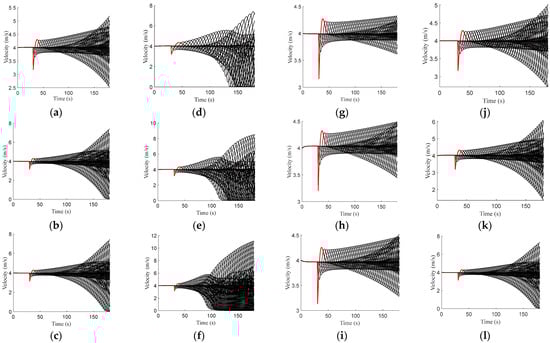
Figure 2. Velocity on a $1000$ m circular road for the ID model with (a) $\delta =1$, (b) $\delta =4$, and (c) $\delta =20$, and the proposed model when $\frac{\tau }{{\tau }_s}<1$ with (d) $h=0.3,$ (e) $h=0.5$, and (f) $h=1.0$, $\frac{\tau }{{\tau }_s}>1$ with (g) $h=0.3$, (h) $h=0.5$, and (i) $h=1.0$, and $\frac{\tau }{{\tau }_s}=1$ with (j) $h=0.3$, (k) $h=0.5$, and (l) $h=1.0$.

For the proposed model with $\frac{\tau }{{\tau }_s}<1$ (aggressive driver), when $h=0.3$, the velocity of the first vehicle decreases to $3.2$ m/s and then increases to $4.3$ m/s at $43.5$ s. At $63.0$ s, it oscillates between $3.5$ and $4.5$ m/s. These oscillations increase over time, and at $178.0$ s, the velocity fluctuates between $0.03$ and $7.3$ m/s as shown in Figure 2d. When $h=0.5$, the velocity of the first vehicle decreases to $3.1$ m/s and then increases to $4.3$ m/s at $40.0$ s. At $50.5$ s, the velocity oscillates between $3.6$ and $4.4$ m/s, and at $179.5$ s, it fluctuates between $0.07$ and $8.5$ m/s as shown in Figure 2e. When $h=1.0$, the velocity of the 1st vehicle decreases to $3.1$ m/s and then increases to $4.3$ m/s at $37.5$ s. At $69.5$ s, the velocity oscillates between $3.1$ and $5.1$ m/s, and at $179.0$ s, it fluctuates between $0.16$ and $11.1$ m/s as shown in Figure 2f.

With $\frac{\tau }{{\tau }_s}>1$ (sluggish driver), at $h=0.3$ the velocity of the $1$st vehicle decreases to $3.1$ m/s and then increases to $4.2$ m/s at $38.0$ s. At $52.0$ s, the velocity oscillates between $3.8$ and $4.2$ m/s, and at $179.5$ s, it fluctuates between $3.6$ and $4.3$ m/s as shown in Figure 2g. When $h=0.5$, the velocity of the $1$st vehicle decreases to $3.2$ m/s and then increases to $4.3$ m/s at $37.5$ s. At $47.5$ s, the velocity oscillates between $3.8$ and $4.2$ m/s, and at $179.5$ s, it fluctuates between $3.4$ and $4.4$ m/s as shown in Figure 2h. When $h=1.0$, the velocity of the $1$st vehicle decreases to 3.1 m/s and then increases to $4.2$ m/s at $38.0$ s. At $55.0$ s, the velocity oscillates between $3.8$ and $4.2$ m/s, and at $179.0$ s, it fluctuates between $3.2$ and $4.5$ m/s as shown in Figure 2i.

With $\frac{\tau }{{\tau }_s}=1$ (typical driver), at $h=0.3$ the velocity of the $1$st vehicle decreases to $3.1$ m/s and then increases to $4.2$ m/s at $38.0$ s. At $47.5$ s, the velocity oscillates between $3.7$ and $4.2$ m/s, and at $179.5$ s, it fluctuates between $2.7$ and $4.9$ m/s as shown in Figure 2j. When $h=0.5$, the velocity of the $1$st vehicle decreases to 3.2 m/s and then increases to $4.3$ m/s at $37.0$ s. At $53.5$ s, the velocity fluctuates between $3.8$ and $4.3$ m/s, and at $179.0$ s, it oscillates between $1.4$ and $6.0$ m/s as shown in Figure 2k. When $h=1$.0, the velocity of the $1$st vehicle decreases to $3.1$ m/s and then increases $\mathrm{to} 4.3$ m/s at $37.0$ s. At $52.0$ s, the velocity fluctuates between $3.7$ and $4.3$ m/s, and at $179.5$ s, it oscillates between $0.04$ and $7.3$ m/s as shown in Figure 2l.

Figure 3 presents the time and space evolution of the vehicles over a circular road of length $1000$ m for the ID and proposed models. This shows the instability that results with both models in the form of stop and go waves. The thick red line represents the $1$st vehicle, while the black lines correspond to the other $20$ vehicles. For the ID model, as $\delta$ increases, the stop and go waves propagate over time and space as shown in Figure 3a,c. For the proposed model, with $\frac{\tau }{{\tau }_s}<1$ (aggressive driver), the stop and go waves are larger, and with $\frac{\tau }{{\tau }_s}>1$ (sluggish driver), they are smaller than with $\frac{\tau }{{\tau }_s}=1$ (typical driver) as shown in Figure 3d,l.

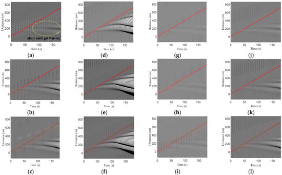
Figure 3. Spatial and temporal vehicle evolution with the ID model for (a) $\delta =1$, (b) $\delta =4,$ and (c) $\delta =20$, and the proposed model for $\frac{\tau }{{\tau }_s}<1$ and (d) $h=0.3$, (e) $h=0.5$, and (f) $h=1.0$, $\frac{\tau }{{\tau }_s}>1$ and (g) $h=0.3$, (h) $h=0.5$, and (i) $h=1.0$, and $\frac{\tau }{{\tau }_s}=1$ and (j) $h=0.3$, (k) $h=0.5$, and (l) $h=1.0$.

The results in Figure 2 and Figure 3 show that with the proposed model, the velocity oscillations are larger for an aggressive driver, and hence, more stop and go waves are produced. This is expected since there are significant interactions between vehicles, which causes congestion [9]. With a sluggish driver, the oscillations are smaller, and hence, fewer stop and go waves are produced. This is because there are fewer interactions between vehicles so the traffic is smooth [9]. The ID model [17] employs a constant exponent $\delta$, which is not based on driver response but rather is a compromise used to characterize all situations. Hence, with the ID model, the velocity oscillations and stop and go waves produced are based on this value, which is inadequate and unrealistic.

4. Simulation Results

The performance of the proposed and ID models is evaluated over a single-lane circular road of length $1200$ m for $150$ s using the explicit Euler method [5] with a time step of $0.5$ s. There are no vehicle exits or entrances on the road. The ID model is evaluated with time headway $2$ s. The proposed model is evaluated with $\tau =1$ s (sensitivity $\frac{\tau }{{\tau }_s}<1$), which corresponds to an aggressive driver, $\tau =2.5$ s (sensitivity $\frac{\tau }{{\tau }_s}>1$), which corresponds to a sluggish driver, and $\tau =2$ s (sensitivity $\frac{\tau }{{\tau }_s}=1$), which corresponds to a typical driver. The value of $h=\frac{s}{D}$ ranges between $0$ and $1$, so here $0.3, 0.5$, and $1.0$ are used. The value of the acceleration exponent $\delta$ varies between $1$ and $\infty$, and is usually $4$ [17], so $\delta =1$, 4, and $20$ are employed. The maximum normalized density is $\frac{1}{s_j}=0.2$ and a platoon of $21$ vehicles is considered. The simulation parameters are given in Table 3.

Table 3. Simulation parameters.

Parameter	Value
Maximum velocity, $v_{max}$	$33.3$ m/s
Maximum acceleration, $a$	$0.73$ m/s2
Minimum acceleration, $b$	$1.67$ m/s2
Jam spacing, $s_j$	$5$ m
Time headway for the ID model, $\tau$	$2$ s
Time headway for the aggressive driver, $\tau$	$1$ s
Time headway for the sluggish driver, $\tau$	$2.5$ s
Time headway for the typical driver, $\tau$	$2$ s
Safe time headway, ${\tau }_s$	$2$ s
Ratio of actual to desired distance headway, $h=\frac{s}{D}$	$0.3, 0.5,$ and $1.0$
Proposed model acceleration, $a$	$1.5$ m/s2
Time step size, $\Delta t$	$0.5$ s
Acceleration exponent, $\delta$	$1, 4$, and $20$
Maximum normalized density, ${\rho }_m=\frac{1}{s_j}$ at $v=0$ m/s	$0.2$
Vehicle length, $l$	$5$ m

Figure 4 presents the flow and velocity with the ID model and the results are summarized in Table 4. When $\delta =1$, the maximum flow is $0.33$ veh/s at a density of $0.03$, and the corresponding velocity is $9.9$ m/s. When $\delta =4$, the maximum flow is $0.42$ veh/s at a density of $0.02$, and the corresponding velocity is $16.9$ m/s. When $\delta =20$, the maximum flow is $0.45$ veh/s at a density of $0.02$, and the corresponding velocity is $27.3$ m/s. Table 4 shows that a smaller value of $\delta$ results in a lower maximum flow and velocity but a larger density. As $\delta$ increases, the maximum flow increases, while the density decreases, whereas the corresponding velocity increases.

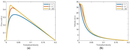
Figure 4. Vehicle behavior with the ID model for $\delta =1, 4,$ and $20,$ (a) flow and (b) velocity.

Table 4. Maximum flow, density, and critical velocity for the ID model.

Acceleration Exponent $\mathit{\delta }$	Maximum Flow (veh/s)	Maximum Density	Critical Velocity (m/s)
$1$	$0.33$	$0.03$	$9.9$
$4$	$0.42$	$0.02$	$16.9$
$20$	$0.45$	$0.02$	$27.3$

Figure 5 presents the flow and velocity with the proposed model for $h=0.3, 0.5,$ and $1.0,$ and the results are summarized in Table 5. With $\frac{\tau }{{\tau }_s}>1$ (aggressive driver), the maximum flow at $h=0.3$ is $0.32$ veh/s at a density of $0.03,$ and the corresponding velocity is $9.4$ m/s. For $h=0.5$, the maximum flow is $0.40$ veh/s at a density of $0.04$, and the corresponding velocity is $10.2$ m/s. For $h=1.0$, the maximum flow is $0.52$ veh/s at a density of $0.05$, and the corresponding velocity is $11.3$ m/s. With $\frac{\tau }{{\tau }_s}>1$ (sluggish driver), the maximum flow at $h=0.3$ is $0.30$ veh/s at a density of $0.03$, and the corresponding velocity is $10.3$ m/s. For $h=0.5$, the maximum flow is $0.33$ veh/s at a density of $0.02$, and the corresponding velocity is 13.2 m/s. For $h=1.0$, the maximum flow is $0.35$ veh/s at a density of $0.02$, and the corresponding velocity is $17.2$ m/s. With $\frac{\tau }{{\tau }_s}=1$ (typical driver), at $h=0.3$, the maximum flow is $0.33$ veh/s at a density of $0.04$, and the corresponding velocity is $9.2$ m/s. For $h=0.5$, the maximum flow is $0.37$ veh/s at a density of $0.03$, and the corresponding velocity is $11.3$ m/s. For $h=1.0$, the maximum flow is $0.41$ veh/s at a density of $0.03$, and the corresponding velocity is $12.1$ m/s. Table 5 indicates that with an aggressive driver, an increase in $h$ increases the maximum flow, density, and velocity. However, with sluggish and typical drivers, an increase in $h$ increases the maximum flow and velocity but decreases the density. Moreover, with an aggressive driver, an increase in $h$ results in a faster increase in the maximum flow compared to a sluggish driver. As expected, with a typical driver the flow and velocity behavior are between the results for aggressive and sluggish drivers.

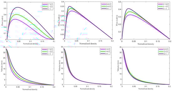
Figure 5. Flow and velocity with the proposed model versus density with $\frac{\tau }{{\tau }_s}<1$, $\frac{\tau }{{\tau }_s}>1$, and $\frac{\tau }{{\tau }_s}=1$ for $h=0.3, 0.5,$ and $1$.

Table 5. Maximum flow, density, and critical velocity for the proposed model.

Driver Sensitivity	$\mathit{h}=\frac{\mathit{s}}{\mathit{D}}$	Maximum Flow (veh/s)	Maximum Density	Critical Velocity (m/s)
$\frac{\tau }{{\tau }_s}<1$ (aggressive driver)	$0.3$	$0.32$	$0.03$	$9.4$
	$0.5$	$0.40$	$0.04$	$10.2$
	$1$.0	$0.52$	$0.05$	$11.3$
$\frac{\tau }{{\tau }_s}>1$ (sluggish driver)	$0.3$	$0.30$	$0.03$	$10.3$
	$0.5$	$0.33$	$0.02$	$13.2$
	$1$.0	$0.35$	$0.02$	$17.2$
$\frac{\tau }{{\tau }_s}=1$ (typical driver)	$0.3$	$0.33$	$0.04$	$9.2$
	$0.5$	$0.37$	$0.03$	$11.3$
	$1$.0	$0.41$	$0.03$	$12.1$

Figure 6 presents the temporal and spatial evolution of a queue for the ID model, and the congestion results are summarized in Table 6. This shows that the velocity within the queue is zero. When $\delta =1$, the queue dissipates at $57.5$ s as shown in Figure 6a, and the corresponding velocity is $1.3$ m/s. When $\delta =4$, the queue dissipates at $56.0$ s as shown in Figure 6b, and the corresponding velocity is $1.2$ m/s. When $\delta =20$, the queue exists from $0$ to $55.5$ s, and the velocity after the queue dissipates varies between $1.1$ and $5.2$ m/s. However, a new queue forms at $84.5$ s and remains until $150.0$ s, spanning $40.0$ to $53.3$ m as shown in Figure 6c. With $\delta =1$, the maximum velocity is $20.0$ m/s, whereas with $\delta =4$ and $20$, it is $25.0$ and $30.0$ m/s, respectively. These results indicate that the traffic queue with the ID model dissipates based on the constant $\delta$ rather than driver response, which is unrealistic.

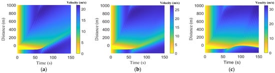
Figure 6. Velocity versus time and space with the ID model over a $1200$ m circular road for (a) $\delta =1$, (b) $\delta =4$, and (c) $\delta =20$.

Table 6. Velocity and time for the ID model during and after congestion.

$\mathbf{Acceleration} \mathbf{Exponent} \mathit{\delta }$	Time during Which Congestion Occurs (s)	Velocity after Congestion Dissipates (m/s)	Time after Congestion Dissipates (s)
$1$	$0-57.5$	$1.3$	$57.5$
$4$	$0-56.0$	$1.2$	$56.0$
$20$	$0-55.5$ and $84.5-150.0$	$1.1-5.2$	$84.5-150.0$

Figure 7 presents the temporal and spatial evolution of a queue with the proposed model, and the congestion results are summarized in Table 7. This shows that the velocity within the queue is zero. For $\frac{\tau }{{\tau }_s}<1$ (aggressive driver), with $h=0.3,$ the queue dissipates at $91.5$ s as shown in Figure 7a, and the corresponding velocity is $1.3$ m/s. With $h=0.5$ and $1.0$, the queue dissipates at $68.0$ and $54.5$ s, respectively, as shown in Figure 7b,c. With $h=0.5$, the velocity after the queue dissipates is $1.6$ m/s, while with $h=1.0$, it is 2.5 m/s. For $\frac{\tau }{{\tau }_s}>1$ (sluggish driver), with $h=0.3$ and $0.5$, the queue dissipates at $62.5$ and $61.0$ s, respectively, as shown in Figure 7d,e. With $h=0.3$, the velocity after the queue dissipates is $1.4$ m/s, while with $h=0.5$, it is $1.2$ m/s. With $h=1.0$, the initial queue dissipates at $60.0$ s and the corresponding velocity is between $1.0$ and $1.9$ m/s as shown in Table 7. A queue again develops at $125.0$ s and lasts until $150.0$ s between $-43.3$ and $-56.6$ m as shown in Figure 7f. For $\frac{\tau }{{\tau }_s}=1$ (typical driver), with $h=0.3$, the queue dissipates at $60.0$ s as shown in Figure 7g, and the corresponding velocity is $1.7$ m/s. With $h=0.5$ and $1.0$, the queue dissipates at $58.5$ and $59.0$ s, respectively, as shown in Figure 7h,i. With $h=0.5$, the velocity after the queue dissipates is $1.8$ m/s, while with $h=1.0$, the velocity is $2.1$ m/s. The largest velocity after the queue dissipates is $2.5$ m/s. These results indicate that queue dissipation is quick with an aggressive driver compared to a sluggish driver. Furthermore, the dissipation with a typical driver is between that of aggressive and sluggish drivers, as expected.

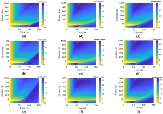
Figure 7. Velocity versus time and space for the proposed model over a $1200$ m circular road for $\frac{\tau }{{\tau }_s}<1$ with (a) $h=0.3,$ (b) $h=0.5,$ and (c) $h=1.0$, $\frac{\tau }{{\tau }_s}>1$ with (d) $h=0.3$, (e) $h=0.5$, and (f) $h=1.0$, and $\frac{\tau }{{\tau }_s}=1$ with (g) $h=0.3$, (h) $h=0.5$, and (i) $h=1.0$.

Table 7. Velocity and time for the proposed model during the queue and after the queue dissipates.

Driver Sensitivity	$\mathit{h}=\frac{\mathit{s}}{\mathit{D}}$	Time during Which Congestion Occurs (s)	Velocity after Congestion Dissipates (m/s)	Time after Congestion Dissipates (s)
$\frac{\tau }{{\tau }_s}<1$ (aggressive driver)	$0.3$	$0-91.5$	$1.3$	$91.5$
	$0.5$	$0-68.0$	$1.6$	$68.0$
	$1.0$	$0-54.5$	$2.5$	$54.5$
$\frac{\tau }{{\tau }_s}>1$ (sluggish driver)	$0.3$	$0-62.5$	$1.4$	$62.5$
	$0.5$	$0-61.0$	$1.2$	$61.0$
	$1.0$	$0-60.0$ and 1$25.0-150.0$	$1.0$ and $1.9$	$60.0$ and $125.0$
$\frac{\tau }{{\tau }_s}=1$ (typical driver)	$0.3$	$0-60.0$	$1.7$	$60.0$
	$0.5$	$0-58.5$	$1.8$	$58.5$
	$1.0$	$0-59$.0	$2.1$	$59.0$

Figure 8 presents the temporal and spatial trajectories of the vehicles with the ID model, and the corresponding congestion results are given in Table 8. The thick red line represents the $1$st vehicle, while the black lines correspond to the other $20$ vehicles. At $55.0$ s, with $\delta =1$, the $1$st vehicle is at $742.0$ m, while the $10$th and $20$th vehicles are at $112.0$ and $-89.9$ m, respectively. With $\delta =4$, the $1$st vehicle is at $919.3$ m, while the $10$th and $20$th vehicles are at $166.4$ and $-88.6$ m, respectively. With $\delta =20$, the $1$st vehicle is at $958.9$ m, while the $10$th vehicle is at $167.6$ m and the $20$th vehicle is at $-88.6$ m. Table 8 indicates that as $\delta$ increases, the distance traveled by the $1$st and $10$th vehicles increases but decreases for the $20$th vehicle.

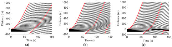
Figure 8. Trajectories of 21 vehicles with the ID model over a $1200$ m circular road for (a) $\delta =1$, (b) $\delta =4$, and (c) $\delta =20$.

Table 8. Position of the $1$st, $10$th, and $20$th vehicles at $55.0$ s with the ID model.

Acceleration Exponent $\mathit{\delta }$	1st Vehicle Position (m)	10th Vehicle Position (m)	20th Vehicle Position (m)
$1$	742.0	112.0	−89.9
4	919.3	166.4	−88.6
20	958.9	167.6	−88.6

The temporal and spatial trajectories of the vehicles with the proposed model are presented in Figure 9 and the corresponding congestion results are given in Table 9. The positions of the $1$st, $10$th, and $20$th vehicles at $55.0$ s are compared. For an aggressive driver, with $h=0.3$, the $1$st vehicle is at $403.4$ m, while the $10$th and $20$th vehicles are at $-11.5$ and $-95.0$ m, respectively. With $h=0.5$, the first vehicle is at $519.3$ m, while the $10$th and $20$th vehicles are at $60.6$ and $-94.9$ m, respectively. With $h=1.0$, the first vehicle is at $683.6$ m, while the $10$th and $20$th vehicles are at $167.6$ and $-77.5$ m, respectively. For a sluggish driver, with $h=0.3$, the $1$st vehicle is at $801.5$ m, while the $10$th and $20$th vehicles are at $95.9$ and $-92.8$ m, respectively. With $h=0.5$, the first vehicle is at $871.1$ m, while the $10$th and $20$th vehicles are at $112.8$ and $-92.7$ m, respectively. With $h=1.0$, the first vehicle is at $923.8$ m, while the $10$th and $20$th vehicles are at $117.9$ and $-92.7$ m, respectively. For a typical driver, with $h=0.3$, the $1$st vehicle is at $720.3$ m, while the $10$th and $20$th vehicles are at $102.6$ and $-90.6$ m, respectively. With $h=0.5$, the first vehicle is at $815.3$ m, while the $10$th and $20$th vehicles are at $141.3$ and $-88.8$ m, respectively. With $h=1.0$, the first vehicle is at $898.5$ m, while the $10$th and $20$th vehicles are at $163.9$ and $-88.6$ m, respectively. Table 9 indicates that for all three driver types, an increase in $h$ increases the position (distance covered) of the 1st and 10th vehicles, whereas the position of the 20th vehicle decreases.

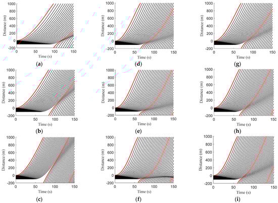
Figure 9. Trajectories of 21 vehicles with the proposed model over a $1200$ m circular road for $\frac{\tau }{{\tau }_s}<1$ with (a) $h=0.3$, (b) $h=0.5$, and (c) $h=1.00$, $\frac{\tau }{{\tau }_s}>1$ with (d) $h=0.3,$ (e) $h=0.5$, and (f) $h=1.0$, and $\frac{\tau }{{\tau }_s}=1$ with (g) $h=0.3$, (h) $h=0.5$, and (i) $h=1.0$.

Table 9. Position of the $1$st, $10$th, and $20$th vehicles at $55.0$ s with the proposed model.

Driver Sensitivity	$$\mathit{h}=\frac{\mathit{s}}{\mathit{D}}$$	1st Vehicle Position (m)	10th Vehicle Position (m)	20th Vehicle Position (m)
$\frac{\tau }{{\tau }_s}<1$ (aggressive driver)	$0.3$	403.4	−11.5	−95.0
	$0.5$	519.3	60.6	−94.9
	1.0	683.6	167.6	−77.5
$\frac{\tau }{{\tau }_s}>1$ (sluggish driver)	$0.3$	801.5	95.9	−92.8
	$0.5$	871.1	112.8	−92.7
	$1.0$	923.8	117.9	−92.7
$\frac{\tau }{{\tau }_s}=1$ (typical driver)	$0.3$	720.3	102.6	−90.6
	$0.5$	815.3	141.3	−88.8
	$1.0$	898.5	163.9	−88.6

Figure 10 presents the traffic flow with the ID model over a $1200$ m circular road for $\delta =1, 4,$ and $20$. This shows that as $\delta$ increases, the variations in the flow also increase. The corresponding flow with the proposed model for $\frac{\tau }{{\tau }_s}<1$ (aggressive driver) is given in Figure 11. This shows that a larger value of $h$ results in smaller variations in flow. Figure 12 and Figure 13 present the flow with the proposed model for $\frac{\tau }{{\tau }_s}>1$ (sluggish driver) and $\frac{\tau }{{\tau }_s}=1$ (typical driver), respectively. These show that the flow is larger with an increase in $h$.

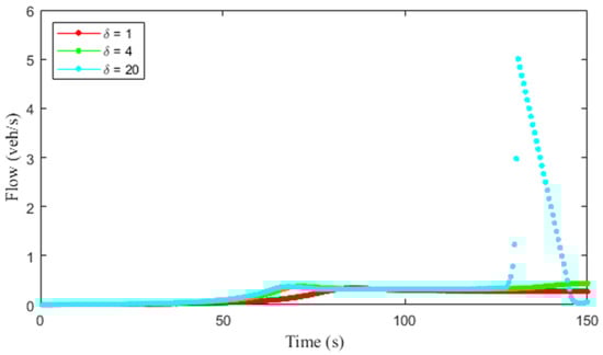
Figure 10. Flow with the ID model for $\delta =1, 4,$ and $20$ over a $1200$ m circular road.

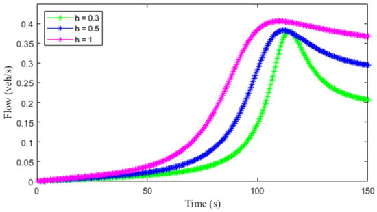
Figure 11. Flow with the proposed model over a $1200$ m circular road for $\frac{\tau }{{\tau }_s}<1$ and $h=0.3, 0.5,$ and $1.0$.

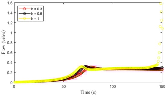
Figure 12. Flow with the proposed model over a $1200$ m circular road for $\frac{\tau }{{\tau }_s}>1$ and $h=0.3, 0.5,$ and $1.0$.

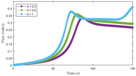
Figure 13. Flow with the proposed model over a $1200$ m circular road for $\frac{\tau }{{\tau }_s}=1$ and $h=0.3, 0.5,$ and $1.0$.

Figure 14 presents the velocity with the ID model over a $1200$ m road for $\delta =1, 4,$ and $20$. This shows that an increase in $\delta$ increases the variations in velocity. The corresponding velocity with the proposed model for $\frac{\tau }{{\tau }_s}<1$ (aggressive driver) is given in Figure 15. This indicates that the variations in velocity are smaller with a larger value of $h$. The velocities with the proposed model for $\frac{\tau }{{\tau }_s}>1$ (sluggish driver) and $\frac{\tau }{{\tau }_s}=1$ (typical driver) are presented in Figure 16 and Figure 17, respectively. These show that the variations in velocity increase with $h$.

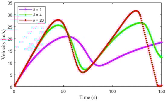
Figure 14. Velocity with the ID model for $\delta =1, 4,$ and $20$ over a $1200$ m circular road.

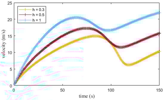
Figure 15. Velocity with the proposed model for $h=0.3, 0.5,$ and $1.0$ with $\frac{\tau }{{\tau }_s}<1$ over a $1200$ m circular road.

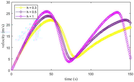
Figure 16. Velocity with the proposed model for $h=0.3, 0.5,$ and $1.0$ with $\frac{\tau }{{\tau }_s}>1$ over a $1200$ m circular road.

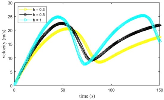
Figure 17. Velocity with the proposed model for $h=0.3, 0.5,$ and $1.0$ with $\frac{\tau }{{\tau }_s}=1$ over a $1200$ m circular road.

Figure 18 presents the density evolution over time and distance with the ID model. When $\delta =1$, the density is $0.012$ from $0$ to $136.5$ m at $149.5$ s. At $336.3$ m, it is $0.03$ and then decreases to $0.016$ at $709.2$ m as shown in Figure 18a. From $0$ to $47.0$ s, there is a traffic queue as the density is $0.20$. At $80.5$ s, the density at $148.0$ s decreases to $0.032$ after the congestion ends. When $\delta =4$, at $147.0$ s the density is $0.014$ from $0$ to $23.3$ m. It increases to $0.036$ at $219.8$ m and then decreases to $0.014$ at $619.4$ m as shown in Figure 18b. From $0$ to $45.0$ s, the density is $0.20$, which indicates a traffic queue. At $149.00$ s, the density decreases to $0.036$. When $\delta =20$, at $147.0$ s the density between $-66.6$ m and $-50.0$ m is $0.20,$ which indicates a traffic queue. At $509.9$ m, it decreases to $0.008$ as shown in Figure 18c. It is $0.20$ from $0$ to $46.5$ s, so there is a traffic queue. The density then decreases to $0.05$ at $66.0$ s. A queue again develops at $77.0$ s as the density is $0.20$ and remains until $150.0$ s between $-66.6$ and $-50.0$ m. Figure 18 shows that as $\delta$ increases, the change in density over time increases, which indicates the model is unstable.

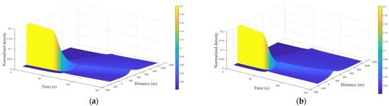
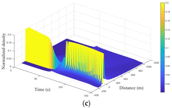
Figure 18. Traffic density with the ID model over a $1200$ m circular road for (a) $\delta =1$, (b) $\delta =4$, and (c) $\delta =20$.

Figure 19 presents the density evolution over time and distance with the proposed model for $\frac{\tau }{{\tau }_s}<1$ (aggressive driver). With $h=0.3$, from $0$ to $53.3$ m at $149.0$ s the density is $0.01$. It increases to $0.06$ at $129.8$ m and then decreases to $0.016$ at $456.2$ m as shown in Figure 19a. From $0$ to $79.0$ s, the density is $0.20,$ which indicates a traffic queue. At $114.5$ s, the queue dissipates and the density decreases to $0.05$ and then increases to $0.06$ at $149.0$ s. With $h=0.5$, from $0$ to $336.3$ m at $148.5$ s, the density is $0.012$. It increases to $0.03$ at $492.8$ m and then decreases to $0.016$ at $885.7$ m as shown in Figure 19b. From $0$ to $49.5$ s, the density is $0.20,$ which indicates a queue, and at $149.0$ s, it decreases to $0.035$. With $h=1.0$, from $0$ to $732.6$ m at $149.5$ s the density is $0.014$. At $985.6$ m it increases to $0.020$ as shown in Figure 19c. From $0$ to $43.0$ s, the density is $0.20$, which indicates a queue. At $146.0$ s, the queue dissipates and the density decreases to $0.015$ at $169.8$ m.

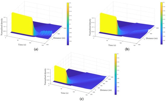
Figure 19. Traffic density with the proposed model over a $1200$ m circular road for $\frac{\tau }{{\tau }_s}<1$ and (a) $h=0.3$, (b) $h=0.5$, and (c) $h=1.0$.

Figure 20 presents the density evolution over time and distance with the proposed model for $\frac{\tau }{{\tau }_s}>1$ (sluggish driver). With $h=0.3$, from $0$ to $26.6$ m, the density is $0.014$ at $149.5$ s. At $150$ s, it is $0.02$ at $329.6$ m and decreases to $0.015$ at $586.0$ m as shown in Figure 20a. From $0$ to $48.5$ s, it is $0.20,$ which indicates a traffic queue, and at $149.0$ s, it decreases to $0.03$. With $h=0.5$, from $0$ to $9.99$ m at $150.0$ s, the density is $0.017$. At $99.9$ m, it increases to $0.038$ and then decreases to $0.014$ at $479.5$ m as shown in Figure 20b. From $0$ to $48.5$ s, it is $0.20$, which indicates a queue, and at $149.0$ s, it decreases to $0.03$. With $h=1.0$, from $-56.6$ to $-43.2$ m at $150.0$ s, the density is $0.20,$ which indicates a queue. It then decreases to $0.012$ at $316.3$ m as shown in Figure 20c. From $0$ to $49.5$ s, the density is $0.20$, which indicates a queue, and at $70.0$ s, it decreases to $0.07$. A queue with density $0.20$ again forms at $131.0$ s and remains until $150.0$ s between $-56.6$ and $-43.2$ m.

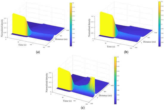
Figure 20. Traffic density with the proposed model over a $1200$ m circular road for $\frac{\tau }{{\tau }_s}>1$ and (a) $h=0.3$, (b) $h=0.5$, and (c) $h=1.0$.

Figure 21 presents the density evolution over time and distance with the proposed model for $\frac{\tau }{{\tau }_s}=1$ (typical driver). With $h=0.3$, from $0$ to $153.2$ m at $150.0$ s, the density is $0.012$. It then decreases to $0.01$ at $526.1$ m as shown in Figure 21a. From $0$ to $43.5$ s, the density is $0.20$, which indicates a queue, and at $147.5$ s, it decreases to $0.032$. With $h=0.5$, from $0$ to $149.8$ m at $150.0$ s, the density is $0.013$. It then increases to $0.029$ at $362.9$ m and decreases to $0.016$ at $729.2$ m as shown in Figure 21b. From $0$ to $46.0$ s, the density is $0.20$, which indicates a queue, and at $148.5$ s, it decreases to $0.03$. With $h=1.0$, from $0$ to $79.9$ m at $149.0$ s, the density is $0.015$ and decreases to $0.013$ at $785.8$ m as shown in Figure 21c. From $0$ to $45.0$ s, the density is $0.20$, which indicates a queue, and it decreases to $0.032$ at $148.0$ s.

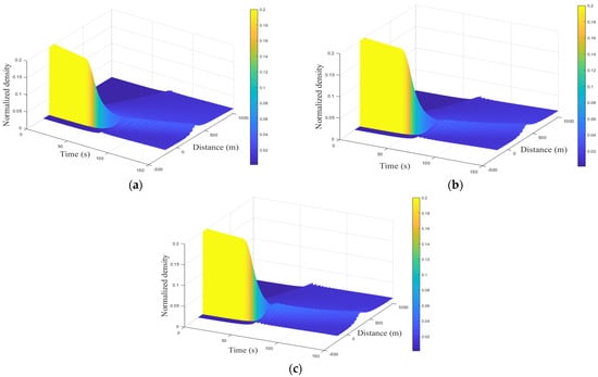
Figure 21. Traffic density with the proposed model over a $1200$ m circular road for $\frac{\tau }{{\tau }_s}=1$ and (a) $h=0.3$, (b) $h=0.5$, and (c) $h=1.0$.

The results presented in this section indicate that with the proposed model and an aggressive driver, the changes in velocity and density are small, but with a sluggish driver, these changes are large. As expected, the response with a typical driver is between that for an aggressive driver and a sluggish driver. However, the ID model employs a fixed exponent regardless of the density and velocity, so the results are unrealistic. Furthermore, vehicle positions are based on a constant rather than the actual and desired distance headways as with the proposed model. Driver sensitivity also affects traffic as movement is faster with an aggressive driver and slower with a sluggish driver. Thus, the proposed model achieves a smooth flow considering driver reaction and sensitivity, which is more realistic than with the ID model. For example, the variations in flow and velocity with the proposed model are greater for a sluggish driver compared to an aggressive driver, as expected.

5. Conclusions

A new microscopic traffic model was introduced which is based on driver response considering both driver reaction and sensitivity. The performance of the proposed model was compared with the well-known ID model over a circular road that can be considered a worst-case scenario. The results obtained show that the density and velocity evolution with the proposed model are realistic as they are based on real traffic parameters. Conversely, the constant exponent used in the ID model produces less realistic results. The proposed model incorporates driver reaction and sensitivity, which generates a smooth traffic flow. Moreover, the variations in flow and velocity are greater with a sluggish driver compared to an aggressive driver, as expected.

The stability results demonstrate that with the proposed model, congestion dissipates quickly with an aggressive driver (large sensitivity). Furthermore, there are larger oscillations in velocity and stop and go waves than with a sluggish driver (small sensitivity), as expected. Hence, the traffic behavior with the proposed model is more stable than with the ID model. This is because the ID model employs a constant exponent $\delta$ to characterize traffic behavior, which is not based on real traffic dynamics.

The proposed model can be integrated into CAVs and ACC systems for efficient and effective traffic management. In addition, it can be used in ADASs to ensure traffic safety by providing information about driver behavior. The proposed model can also be employed in ADSs for realistic traffic characterization.

References

- Khan, Z.H.; Gulliver, T.A.; Khattak, K.S.; Qazi, A. A macroscopic traffic model based on reaction velocity. Iran. J. Sci. Technol. Trans. Civ. Eng. 2020, 44, 139–150. [Google Scholar] [CrossRef]
- Khan, Z.H.; Imran, W.; Azeem, S.; Khattak, K.S.; Gulliver, T.A.; Aslam, M.S. A macroscopic traffic model based on driver reaction and traffic stimuli. Appl. Sci. 2019, 9, 2848. [Google Scholar] [CrossRef]
- Kerner, B.S.; Klenov, S.L. A theory of traffic congestion at moving bottlenecks. J. Physics A Math. Theor. 2010, 43, 425101. [Google Scholar] [CrossRef]
- Long, J.; Gao, Z.; Ren, H.; Lian, A. Urban traffic congestion propagation and bottleneck identification. Sci. China F Inform. Sci. 2008, 51, 948–964. [Google Scholar] [CrossRef]
- Kessels, F. Traffic Flow Modelling: Introduction to Traffic Flow Theory through a Genealogy of Models; Springer: Cham, Switzerland, 2019. [Google Scholar]
- Wang, J.; Chai, R.; Xue, X. The effects of stop-and-go wave on the immediate follower and change in driver characteristics. Procedia Eng. 2016, 137, 289–298. [Google Scholar] [CrossRef]
- Khan, Z. Traffic Modelling for Intelligent Transportation Systems. Ph.D. Dissertation, University of Victoria, Victoria, BC, Canada, 2016. [Google Scholar]
- Khan, Z.H.; Gulliver, T.A. A macroscopic traffic model based on anticipation. Arab. J. Sci. Eng. 2019, 44, 5151–5163. [Google Scholar] [CrossRef]
- Khan, Z.H.; Gulliver, T.A.; Khattak, K.S. A novel macroscopic traffic model based on distance headway. Civ. Eng. J. 2021, 7, 32–40. [Google Scholar] [CrossRef]
- Henein, C.M.; White, T. Microscopic information processing and communication in crowd dynamics. Phys. A Stat. Mech. Appl. 2010, 389, 4636–4653. [Google Scholar] [CrossRef]
- Ali, F.; Khan, Z.H.; Khan, F.A.; Khattak, K.S.; Gulliver, T.A. A new driver model based on driver response. Appl. Sci. 2022, 12, 5390. [Google Scholar] [CrossRef]
- Ali, F.; Khan, Z.H.; Khattak, K.S.; Gulliver, T.A.; Khan, A.N. A microscopic heterogeneous traffic flow model considering distance headway. Mathematics 2023, 11, 184. [Google Scholar] [CrossRef]
- Ali, F.; Khan, Z.H.; Khan Khattak, K.S.; Gulliver, T.A. A microscopic traffic flow model characterization for weather conditions. Appl. Sci. 2022, 12, 12981. [Google Scholar] [CrossRef]
- Khan, Z.H.; Gulliver, T.A.; Nasir, H.; Rehman, A.; Shahzada, K. A macroscopic traffic model based on driver physiological response. J. Eng. Math. 2019, 115, 21–41. [Google Scholar] [CrossRef]
- Gazis, D.C.; Herman, R.; Rothery, R.W. Nonlinear follow-the-leader models of traffic flow. Oper. Res. 1961, 9, 545–567. [Google Scholar] [CrossRef]
- Newell, G.F. Nonlinear effects in the dynamics of car following. Oper. Res. 1961, 9, 209–229. [Google Scholar] [CrossRef]
- Treiber, M.; Hennecke, A.; Helbing, D. Congested traffic states in empirical observations and microscopic simulations. Phys. Rev. E 2000, 62, 1805–1824. [Google Scholar] [CrossRef] [PubMed]
- Bando, M.; Hasebe, K.; Nakayama, A.; Shibata, A.; Sugiyama, Y. Dynamical model of traffic congestion and numerical simulation. Phys. Rev. E 1995, 51, 1035–1042. [Google Scholar] [CrossRef]
- Krautter, W.; Bleile, T.; Manstetten, D.; Schwab, T. Traffic simulation with ARTIST. In Proceedings of the Conference on Intelligent Transportation Systems, Boston, MA, USA, 9–12 November 1997. [Google Scholar]
- Helbing, D.; Tilch, B. Generalized force model of traffic dynamics. Phys. Rev. E 1998, 58, 133–138. [Google Scholar] [CrossRef]
- Gipps, P.G. A behavioural car-following model for computer simulation. Transp. Res. Part B 1981, 15, 105–111. [Google Scholar] [CrossRef]
- Cao, Z.; Lu, L.; Chen, C.; Chen, X.U. Modeling and simulating urban traffic flow mixed with regular and connected vehicles. IEEE Access 2021, 9, 10392–10399. [Google Scholar] [CrossRef]
- Dahui, W.; Ziqiang, W.; Ying, F. Hysteresis phenomena of the intelligent driver model for traffic flow. Phys. Rev. E 2007, 76, 2–8. [Google Scholar] [CrossRef] [PubMed]
- Kesting, A.; Treiber, M.; Helbing, D. Enhanced intelligent driver model to access the impact of driving strategies on traffic capacity. Philos. Trans. R. Soc. A Math. Phys. Eng. Sci. 2010, 368, 4585–4605. [Google Scholar] [CrossRef]
- Liebner, M.; Baumann, M.; Klanner, F.; Stiller, C. Driver intent inference at urban intersections using the intelligent driver model. In Proceedings of the IEEE Intelligent Vehicle Symposium, Madrid, Spain, 3–7 June 2012. [Google Scholar]
- Derbel, O.; Peter, T.; Zebiri, H.; Mourllion, B.; Basset, M. Modified intelligent driver model for driver safety and traffic stability improvement. IFAC Proc. 2013, 46, 744–749. [Google Scholar] [CrossRef]
- Li, y.; Li, Z.; Wang, H.; Wang, W.; Xing, L. Evaluating the safety impact of adaptive cruise control in traffic oscillations on freeways. Accid. Anal. Prev. 2017, 104, 137–145. [Google Scholar] [CrossRef]
- Schakel, W.J.; van Arem, B.; Netten, B.D. Effects of cooperative adaptive cruise control on traffic flow stability. In Proceedings of the International IEEE Conference on Intelligent Transportation Systems, Funchal, Portugal, 19–22 September 2010. [Google Scholar]
- Jafaripournimchahi, A.; Cai, Y.; Wang, H.; Sun, L.; Weng, J. Integrated-hybrid framework for connected and autonomous vehicles microscopic traffic flow modelling. J. Adv. Transp. 2002, 2022, 2253697. [Google Scholar] [CrossRef]
- Tapani, A. Traffic simulation modelling of driver assistance systems. Adv. Transp. Stud. 2011, 1, 41–50. [Google Scholar]
- Mazzega, J.; Lipinski, D.; Eberle, U.; Schittenhelm, H.; Wachenfeld, W. PEGASUS Method. Zenodo 2019, 2019, 6595201. [Google Scholar] [CrossRef]
- Krajzewicz, D.; Hertkorn, G.; Feld, C.; Wagner, P. SUMO (Simulation of Urban MObility) An open-source traffic simulation. In Proceedings of the Middle East Symposium on Simulation and Modelling, Sharjah, United Arab Emirates, 28–30 September 2002. [Google Scholar]
- Salles, D.; Kaufmann, S.; Reuss, H. Extending the intelligent driver model in SUMO and verifying the drive off trajectories with aerial measurements. In Proceedings of the SUMO User Conference, Online, 26–28 October 2020. [Google Scholar]
- Kokuti, A.; Hussein, A.; Marín-Plaza, P.; de La Escalera, A.; García, F. V2X communications architecture for off-road autonomous vehicles. In Proceedings of the IEEE International Conference on Vehicular Electronics and Safety, Vienna, Austria, 27–28 June 2017. [Google Scholar]
- PTV Group. PTV Vissim Multimodal Traffic Simulation Software. Available online: https://www.myptv.com/en/mobility-software/ptv-vissim (accessed on 30 August 2022).
- Liu, P.; Fan, W. Exploring the impact of connected and autonomous vehicles on freeway capacity using a revised intelligent Driver Model. Transp. Plan. Technol. 2020, 43, 279–292. [Google Scholar] [CrossRef]
- Hallerbach, S.; Xia, Y. Simulation-based identification of critical scenarios for cooperative and automated vehicles. SAE Int. J. Connect. Autom. Veh. 2018, 1, 93–106. [Google Scholar] [CrossRef]
- U.S. Department of Transportation. Next Generation Simulation (NGSIM) Vehicle Trajectories and Supporting Data. Available online: https://datahub.transportation.gov/Automobiles/Next-Generation-Simulation-NGSIM-Vehicle-Trajector/8ect-6jqj/data (accessed on 5 May 2023).
- Xia, X.; Meng, Z.; Han, X.; Li, H.; Tsukiji, T.; Xu, R.; Zheng, Z.; Ma, J. An automated driving systems data acquisition and analytics platform. Transp. Res. Part C Emerg. Technol. 2023, 151, 104120. [Google Scholar]
- Dosovitskiy, A.; Ros, G.; Codevilla, F.; López, A.; Koltun, V. CARLA: An open urban driving simulator. In Proceedings of the Annual Conference on Robot Learning, Mountain View, CA, USA, 13–15 November 2017. [Google Scholar]
- Imran, W.; Khan, Z.H.; Gulliver, T.A.; Khattak, K.S.; Nasir, H. A macroscopic traffic model for heterogeneous flow. Chin. J. Phys. 2020, 63, 419–435. [Google Scholar] [CrossRef]
- Askari, A.; Farias, D.A.; Kurzhanskiy, A.A.; Varaiya, P. Measuring impact of adaptive and cooperative adaptive cruise control on throughput of signalized intersections. arXiv 2017, arXiv:1611.08973. [Google Scholar]
- Hellinga, B.R. Requirements for the calibration of traffic simulation models. Proc. Can. Soc. Civ. Eng. 1998, 4, 211–222. [Google Scholar]
- Liu, W.; Xia, X.; Xiong, L.; Lu, Y.; Gao, L.; Yu, Z. Automated vehicle sideslip angle estimation considering signal measurement characteristic. IEEE Sens. J. 2021, 21, 21675–21687. [Google Scholar] [CrossRef]
- Treiber, M.; Kesting, A. Traffic Flow Dynamics: Data, Models and Simulation; Springer: Berlin, Germany, 2013. [Google Scholar]
- Feng, S.; Zhang, Y.; Li, S.E.; Cao, Z.; Liu, H.X.; Li, L. String stability for vehicular platoon control: Definitions and analysis methods. Ann. Rev. Control 2019, 47, 81–97. [Google Scholar] [CrossRef]
Disclaimer/Publisher’s Note: The statements, opinions and data contained in all publications are solely those of the individual author(s) and contributor(s) and not of MDPI and/or the editor(s). MDPI and/or the editor(s) disclaim responsibility for any injury to people or property resulting from any ideas, methods, instructions or products referred to in the content. |
© 2023 by the authors. Licensee MDPI, Basel, Switzerland. This article is an open access article distributed under the terms and conditions of the Creative Commons Attribution (CC BY) license (https://creativecommons.org/licenses/by/4.0/).