Abstract
Most granular flow in nature and industrial processing has the property of polydispersity, whereas we are always restricted to using the monodisperse drag force model in simulations since the drag force model with polydispersity is difficult to establish. Ignoring polydispersity often results in obvious deviations between simulation and experimental outcomes. Generally, it is very hard for us to describe the characteristics of polydispersity in drag force by using a function with analytic expression. Recently, the artificial neural network (ANN) model provides us the advantages of estimating these kinds of outcomes with better accuracy. In this work, the ANN is adopted to model the drag force in polydisperse granular flows. In order to construct a reasonable ANN algorithm for modeling the polydisperse drag force, the structures of ANN are elaborately designed. As training for the ANN drag model, a direct numerical simulation method is proposed, based on the lattice Boltzmann method (LBM), to generate the training data, and an adaptive data filtering algorithm, termed as the optimal contribution rate algorithm (OCRA), is introduced to effectively improve the training efficiency and avoid the over-fitting problems. The results support that the polydispersity of the system can be well scaled by the ANN drag model in a relatively wide range of particle concentrations, and the predicted results coincide well with the experimental ones. Moreover, the ANN drag model is not only effective for polydisperse systems, but compatible with monodisperse systems, which is impossible using traditional drag models.
1. Introduction
Most granular flows encountered in daily life and industrial processing have polydisperse characteristics [1,2,3,4,5,6,7], for instance, drug production, coal gasification, haze control, and sandstorm prevention [8,9]. The polydisperse gas–solid system, compared with the monodisperse counterpart, usually contains particles with different sizes and demonstrates heterogeneous characteristics [10,11,12]. Generally, the drag force of polydisperse systems, which is very important to the discrete element method (DEM) simulations [13,14,15,16,17], is substantially different from that of the monodisperse systems [18,19,20]. The polydispersity has been recognized as one of the most important factors that greatly affects the fluidization state of the granular system [21]. Accordingly, the drag force model for the monodisperse system is no longer applicable for polydisperse systems [22,23].
In recent years, there have been many important studies on the drag force models of polydisperse granular systems. In 2005, van der Hoef et al. [24] extended the monodisperse drag force model of Hill et al. [25] to polydisperse granular systems by introducing a corrected volume fraction, a diameter fraction, and the Sauter mean diameter. In 2006, Benyahia et al. [26] extended the applicability for the Hill et al. formula [25] in a wider range of the Reynolds number. In 2007, Beetstra et al. [27] indicated that the linear dependence on the Reynolds number in the Ergun drag force model [28] is insufficient, and revised the model subsequently by using the direct simulation data that were obtained by the lattice Boltzmann method (LBM). Subsequently, the drag model of polydisperse granular flow with Gaussian and log-normal distribution was constructed by Sarkar et al. in 2009 [29]. However, the above models are only applicable to some high and moderate void fraction flow systems. For low void fraction and moderate-to-high Reynolds number flow systems, these models have not been thoroughly verified yet.
To improve the applicability of the drag force models in the polydisperse granular systems, Holloway and Sundaresan [30] and Yin et al. [31] made further corrections based on the work of van der Hoef et al. [24] and Beetstra et al. [27]. Compared with Yin et al.’s work [31], Cello et al. [14] gave a more concise and unified model by using the data from [24,31]. It has been verified that these improvements can give good predictions for bi-disperse granular systems, but it is not confirmed that these models are applicable to polydisperse granular systems mixed with three or more kinds of granules [15]. For more general cases, Rong et al. considered the particle size distribution in their model, where the data were obtained by using LBM simulations [32]. In 2019, Qin et al. [22] derived a polydisperse energy-minimization multiscale (EMMS) drag model by dividing the systems into three particle phases and considering each phase separately.
Although a lot of important progress has been achieved in modeling the drag force for polydisperse granular flows, there are still some drawbacks that need to be addressed and improved. Firstly, the samples used in building the drag models are few and mainly derived from bi-disperse granular systems. Secondly, most drag models are only applicable to dilute phase systems with a large void fraction. Thirdly, these polydisperse drag models are in general not compatible with monodisperse systems. In view of these drawbacks, this paper establishes a new drag model for polydisperse granular flows by using a supervised machine learning approach. More samples will be used in the proposed model, so that it can be applied to dense phase systems and be compatible with monodisperse systems.
So far, much attention has been paid to the supervised machine learning approach in modeling the granular drag force. Jiang et al. [33] scaled the drag force applied in a filtered two-fluid model (TFM) by using the slip velocity predicted by an artificial neural network (ANN). Only the datasets obtained from the simulation of the bubbling fluidized beds containing bubble-dominated meso-scale structures were employed in training the network; therefore, the resulting model may not be suitable for flows in other regimes. He and Tafti [34] used ANN to build the drag force model for polydisperse spherical granules; besides a solid fraction and Reynolds number, the relative neighboring granule locations are also considered as new inputs in the ANN to improve the predicted capability of the model. Yet, the model’s applicable range is only in a low-intermediate Reynolds number and low solid fraction in a polydisperse granular system. Further, Zhu et al. [35] compared the performance of two different machine learning models, ANN and eXtreme gradient boosting (Xgboost), in predicting the drag force between interphases in a filtered sub-grid model (SGM). They found that the Xgboost model is more suitable for fewer training samples, while the ANN is more suitable for adequate training samples. In 2020, Zhang et al. [36] applied the convolutional neural network (CNN) to predict the drag force in a filtered TFM. They found the information (e.g., Reynolds stress and solid phase stress) from the neighboring coarse grids is of great significance in improving the accuracy. Luo et al. [37] modeled the drag force in deep bubbling beds by using ANN with the data obtained from the immerse boundary method. Besides the Reynolds number and solid volume fraction, two new inputs, the velocity fluctuation and position fluctuation of granules, were introduced to the ANN to improve the accuracy of the model. Compared to Tang’s drag model [38], their model can give better predictions for monodisperse granular systems. In 2022, Ashwin et al. [39] used CNN to study three types of ellipsoidal granules; the training data are obtained from particle resolved simulations (PRSs), but the solid fraction of the drag model is 0.1–0.3, and the applicable range of the model is limited in bubbling fluidized beds. In 2023, Hwang et al. [40] used deep learning techniques to study the drag force of polydisperse irregular-shaped granules in particle-laden flow; the applicable range of the model was expanded to an intermediate Reynolds number incompressible flow compared to their previous work [41]. Whereas their drag model still mainly focused on dilute polydisperse flows, the applicability in a dense monodisperse granular flow has not been verified yet. Beyond that, there are still other works associated with the drag force based on ANN [42,43,44].
The above studies took full advantage of ANN in self-learning and high compatibility during modeling of the drag force. Compared with the classical mathematical analysis approaches, the ANN can learn complex nonlinear relationships from the datasets spontaneously. It has the advantages of flexible structure, simple algorithm, self-learning ability, and good compatibility [45]. The strong predictive capabilities of ANN in modeling the drag force have been well demonstrated in the present studies. However, the models given by these studies still have three imperfections. First, these polydisperse models are applicable in the relatively dilute low-intermediate Reynolds number flow systems; they can scarcely be adopted in a relatively dense granular system. Second, these polydisperse drag models are hardly compatible with a monodisperse granular system since the training samples were mainly from the direct simulations of polydisperse granular systems. Third, the polydisperse drag model suffers from low computational efficiency and over-fitting problems because of the huge training sample set; these studies rarely focus on the training strategy to improve the computational efficiency and avoid over-fitting problems. So, the primary objective of this paper is to extend the applicability of the ANN drag model and improve its computational efficiency. The original contribution of this paper can be drawn in three points. To start with, the drag model with wide applicability in a solid fraction is proposed by using ANN techniques. Next, the proposed ANN drag model is not only applicable in a polydisperse granular system, but has good prediction accuracy in a monodisperse granular system. Finally, a new adaptive data filtering algorithm based on the conception of a contribution rate to improve the training efficiency and avoid over-fitting problems is proposed, so that the redundant samples and singular samples are automatically eliminated from the training set.
The paper is organized as follows. In Section 2, we introduce the numerical method for generating the dataset and how to split it. In Section 3, the structure and parameters of the ANN for the polydisperse drag model are discussed, and an efficient and accurate algorithm that has the adaptive characteristics for training the ANN drag model is proposed. Subsequently, in Section 4, the developed model is compared with the Beestra et al. (BVK) [27], Cello et al. [21], and Holloway and Sundaresan (HS) formula [30] to demonstrate the validity, feasibility, and practicability of the model. Finally, some concluding remarks are given in Section 5.
2. Numerical Method for Dataset Generation
2.1. Numerical Method
LBM, as a mesoscopic method, can be considered as a numerical method independent of continuous kinetic theory. Compared with traditional macroscopic numerical methods, LBM has the advantages of easy coding implementation [46], good parallelism, easily handled geometrically complicated boundaries, and accurately describing the macroscopic motion phenomenon between gas–solid two phases at the microscopic level [46,47]. Therefore, LBM is suitable for the polydisperse system of granular flow by considering its computational accuracy and efficiency of large complex fluid systems.
So far, LBM is widely adopted as a solver to describe the characteristics of granular flow in which rigid granules are immersed in the continuum Newtonian fluid. In this context, we start with the Navier–Stokes equation, which is described by the lattice Boltzmann equation [48] as:
where is the distribution function with discrete velocity at a position and a time , is the time step size, is the total number of discrete velocities, and is the relaxation time. is the equilibrium distribution function, which depends on the density , velocity , and temperature of the fluid. [48] can be described as:
where is the model-dependent weight coefficient, ( is the gas constant) is the lattice sound velocity. The fluid density and velocity can be derived as the zero-th and first order moments of , respectively, as:
The fluid pressure is defined directly as . Through the Chapman–Enskog expansion, the Navier–Stokes equations can be obtained with the viscosity [49] given by:
According to the definition of the Reynolds number , the relaxation time [50] is calculated by:
where and are the characteristic velocity and length, respectively.
To obtain the drag force of a polydisperse system of granular flow, the structure of a polydisperse granular cluster in the flow field was randomly generated. Regarding the boundary condition, our model was referred to the LBM model of Chen et al. [51]. The inlet boundary condition of the fluid field was set to the constant velocity, which was U = 0.1 m/s. At the outlet boundary, a stress-free condition was set, and the periodic boundary conditions were applied to the other two directions. For these settings, as shown in Figure 1, the flows horizontally from left to right with a steady state were gradually achieved, which means the flow field reaches the equilibrium state at each moment.
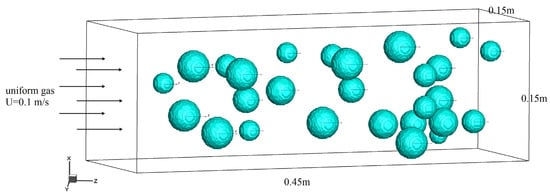
Figure 1.
The sketch of polydisperse system of granular flow.
Considering our previous study [23], a grid was employed, and a single-relaxation-time collision operator in conjunction with a D3Q19 lattice was adopted for the accuracy and stability of the model. In order to improve the computational efficiency of a polydisperse system, a parallel algorithm (MPI+LBM) was used to implement the numerical simulation in the flow field. An in-house C++ LBM solver developed by our research group was used, and the parameters of direct numerical simulation (DNS) [52] are listed in Table 1.

Table 1.
The DNS parameters.
Given the advantages of a simple calculation process, ease of programming, and good prediction accuracy in particle-suspended flow, the momentum exchange method [53] is adopted to calculate the drag force. Specifically, the drag force that acts on the solid surface is obtained by calculating the momentum exchange on each boundary link between each two opposing directions of the neighboring nodes as:
where , are the fluid node and its neighboring solid node, respectively, and .
For training the ANN, the particle Reynolds number [20] is calculated by
where
with is the gas instantaneous velocity in the position of an individual granule, is the solid velocity; in the simulation, the solid velocity was set to zero. is the solid volume fraction. is the Sauter mean diameter [54], which is defined as:
The solid volume fraction [20] is the ratio of the volume of the granular cluster to the grid volume occupied by the granular cluster and can be represented as:
and the void fraction as:
Table 2 presents the average drag force of the granules calculated by the LBM model when the void fraction . Moreover, the scaling of the dimensionless average drag coefficient is the drag force acting on a single granule in the flow field under . The diameter of a single granule is 12. After comparison, the simulation results are consistent with the published literature [19].
Table 2.
Dimensionless drag of granules calculated by 3D LBM when .
2.2. Dataset Splitting
In the 3-dimensional (3D) LBM model, 450 granules were randomly generated per simulation, and approximately 430 simulations were conducted. Then, 80% of the total 243,260 training data with Re = 0.01 to 1100 is obtained in the simulation. The information for each granule after simulation will be grouped in a set . Overall, 17% of the total training data is acquired from Ref. [24] for a monodisperse system with , and the other 3% is obtained from Ref. [25] for a monodisperse system with .
The dataset is composed of the samples for the monodisperse system and polydisperse system of granules. The void fraction range of the granular system is . To ensure a large diversity of shapes, 5 sizes of granules (see Table 1) are randomly distributed in and , then the dataset is systematically divided into 3 subsets: 70% of samples for the training set, 15% of samples for the validation set, and 15% of samples for the testing set. If the ANN model appears to have over-fitting problems during the prediction step, a filtering algorithm will be adopted to avoid it.
The training dataset is used for training the ANN model, the validation dataset is for fine-tuning the hyperparameters of the model, [55] and the testing dataset is for evaluating the trained model performance. It should be noted that there are no intersections among the three datasets, which ensures that the testing dataset will reflect the generalization performance of the model on invisible data.
3. ANN Drag Model and Training Strategy
3.1. The Construction of ANN
A proper design of the ANN structure can greatly improve the computing efficiency and prediction accuracy of the neural network. In order to obtain a reasonable ANN frame for modeling the drag force, the learning algorithm, activation function, hidden layers, and input variables of ANN will be discussed based on the TensorFlow to build the patterning drag model.
As the 243,260 training samples are the local drag forces for each individual granule, it is worth noting that with the changes of sampling location and time, the local drag force will be changed obviously. Moreover, the mesoscale heterogeneity, particle motion characteristics, fluid–solid density ratio, and other factors may affect the simulation results substantially. Thus, it is necessary to preprocess local drag force data by statistical averaging methods, hoping to eliminate the influence of statistical fluctuation that is caused by incomplete consideration of influencing factors.
The local drag forces were grouped in the 2-dimensional interval (, ), with an interval size of and . The average local drag forces [56] were calculated in each interval by:
where represents the number of data in the interval (, ), with an interval size of and . After local drag force averaging, 66,000 samples are left.
Due to the particle Reynolds number , the solid volume fraction and slip velocity , which are used to characterize the movement characteristics of particles, have clear physical meaning and an explicit relationship with drag force [19]. Thus, the above variables will be chosen as the inputs of the ANN drag model. Moreover, the Sauter mean diameter is selected as the input, considering the description of the polydisperse characteristics in the ANN drag model. The input–output variables relationship of the ANN is illustrated in Figure 2.
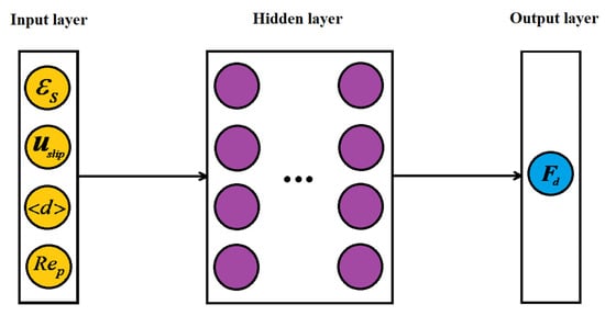
Figure 2.
ANN structure of polydisperse drag model.
3.1.1. The Learning Algorithm of ANN Drag Model
Since the gradient descent with momentum (GDM) algorithm and the Levenberg–Marquardt (LM) algorithm are the commonly used learning algorithms in ANN [45], we decided to compare their performance on the convergence of ANN. Two termination rules, “rule A”, which gives the maximum number of iterations, and “rule B”, which is the given error tolerance, are adopted simultaneously. To reduce the impact of the random initialization of weights, we conducted three independent experiments and recorded the mathematical expectation of the Spearman correlation coefficient [57] between the outputs and the expected outputs in Table 3. It can be found that LM has more accurate prediction results in terms of convergence and applicability compared to the GDM algorithm. However, GDM has advantages of computational efficiency in simulations. Considering the principle of precision priority in designing the ANN, the LM algorithm will be adopted as the learning algorithm of ANN.
Table 3.
Spearman correlation coefficient and CPU time for two training algorithms.
3.1.2. The Activation Function
Different activation functions have various ranges of influence on the prediction accuracy of the ANN; thus, it is necessary to discuss the performance of commonly used activation functions, including Sigmoid, Tanh, Leaky-LU, and Gauss. The predicted results of ANN with a single hidden layer under three independent experiments are illustrated in Table 4.
Table 4.
Comparison of activation functions of 1 hidden layer with 15 neurons.
There is an obvious difference in computational accuracy among the four activation functions. Specifically, the Leaky-LU function demonstrates the lowest prediction accuracy compared to the Tanh function and the Sigmoid function. The prediction results of the Gauss function for the three independent experiments show significant differences. Considering the characteristics of the Gauss activation function, this may be caused by its local response property [45]. Therefore, it is suggested to avoid using it to build the polydisperse drag force model. Moreover, the Sigmoid and Tanh activation functions have a similar prediction accuracy, and both belong to the so-called “S-function”. Because the Tanh function shows a symmetry property with the origin point in the Cartesian coordinate system, it will be beneficial to be utilized for preserving the original properties of the parameters [45]. Consequently, it is more reasonable to use the Tanh function as the activation function in modeling the drag force.
3.1.3. The Structure of Hidden Layers
The structure of the hidden layers is an important factor that influences the ANN performance. Montavon et al. [45] have proved that a one-hidden-layer back-propagation (BP) neural network can realize arbitrary nonlinear mapping. Thus, we will first discuss the influence of the number of hidden layers on the convergence speed and accuracy of the neural network with a multi-hidden-layer structure, as shown in Figure 2.
The independent experimental results of an ANN with one, two, three, and four hidden layers are given in Table 5. It is found that the calculation time and number of iterations increase as the number of hidden layers increases. Accordingly, considering the prediction accuracy and efficiency of ANN, the single hidden layer is preferred in modeling the drag force.
Table 5.
Comparison of the number of hidden layers for ANN’s experimental results.
Next, we will discuss the influence of the structure and the number of neurons in the single hidden layer of the ANN on the convergence speed, correlation coefficient, and CPU time. We took the average results of three independent experiments and recorded them in Table 6. It can be found that considering the influence of the number of neurons on the correlation coefficient and CPU time, a single-hidden-layer BP neural network with 15 neurons is suggested to be implemented for the current study. Moreover, the impacts of input and output correlations for ANN are illustrated in Appendix A.
Table 6.
Comparison of the number of neurons in single hidden layer.
Finally, the conclusion can be drawn that the Levenberg–Marquardt (LM) algorithm is recommended as the learning method, and a single hidden layer with a 15-neurons back-propagation (BP) neural network attached to the Tanh activation function is suggested during the construction of the polydisperse granular drag force model.
3.2. The Optimal Contribution Rate Algorithm (OCRA)
The ability of ANN to explore the correlation between variables is not limitless [45], and the predicted results depend significantly on the correlation between inputs and outputs. When the input samples corresponding to the output variable are incomplete and the relationship between them is not clear, it will bring great challenges to the ANN. Thus, an additional preprocessing method may be required when the correlation between the inputs and outputs is found to be ambiguous.
In the applications of the ANN-machine learning model, various fitting problems are encountered due to diverse functional realizations. In order to complete the prediction of some complex nonlinear relationships, a huge training sample set is required to construct a precise ANN prediction model. However, the huge training sample set will bring a significant reduction in the training and computing efficiency of the ANN. The reason is that according to the characteristics of the ANN-machine learning model, it is prone to result in repeated and inefficient training for ANN by using the linearly correlated training samples (i.e., inefficient training samples). Meanwhile, the training samples with the property of mutual independence (i.e., efficient training samples) are more preferable [45]. Considering that the huge training sample set for the complex nonlinear relationships contains the efficient and inefficient training samples, it is necessary to design an algorithm that can identify the different types of training samples and search for the most efficient one for training. For this purpose, we will propose an adaptive data filtering algorithm, i.e., the OCRA. The implementation of the algorithm can be divided into two steps. The first step is to analyze the contribution rate of the training samples inspired by the idea of the kernel principal component analysis (KPCA) [58]. The second step is to search for an optimal training sample set adaptively with the best contribution rate according to the certain tolerance of the training error.
3.2.1. Contribution Rate Analysis Algorithm
We assume that the input samples in the training model of ANN are represented by:
where denotes the j-th input sample
where represents the i-th index of the j-th input sample. The process of obtaining the data contribution rate and the cumulative contribution rate of training samples is divided into four steps:
- (I)
- Considering the logarithmic characteristics of drag distribution in the polydisperse gas–solid system (see Table 2) and the following contribution rate analysis, in which the input data are required by principal component analysis to maintain a standardized and linear property [58,59], we propose a kernel function to process the input samples as follows:In the above formula, is the j-th sample of the i-th index after that the original matrix was standardized and linearized. is the statistical average of the i-th sample, and is the standard deviation of the i-th sample.
- (II)
- To explore the independence between training samples, we need to construct the covariance matrix of the standardized sample set [57] as:
- (III)
- Perform similarity transformations on the covariance matrix and calculate the eigenvalues of the covariance matrix to demonstrate the property of independence for each training sample [60]whereis a diagonal matrix with the eigenvalues of matrix .
- (IV)
- Finally, the contribution rate and the cumulative contribution rate of the training sample and training sample set will be calculated by
Through the above four steps, we can obtain the contribution rate and the cumulative contribution rate of the training sample and training sample set.
3.2.2. Adaptive Searching of Optimal Contribution Rate
In the previous section, we have introduced the concept of the contribution rate of the training samples. To effectively improve the training efficiency in the certain error tolerance, it needs to analyze the training sample set and use the most valuable information to train the ANN. Meanwhile, some samples with a low contribution rate need to be excluded from the training. In view of these, an adaptive searching method of the optimal contribution rate for the training dataset needs to be designed; it is hoped to maximize the computational efficiency of the ANN within the given error tolerance of the system.
To establish the adaptive searching algorithm of the optimal contribution rate in the training dataset, the basic idea of the bisection algorithm for solving nonlinear equations is employed. The algorithm can be divided into four steps:
(I) First, set the error tolerance of the system as:
Since the mean square error (MSE) has the approximate growing trend with the mean absolute error (MAE) and mean relative error (MRE) in the data fitting, and can better demonstrate the degree of errors dispersion of the predicted results, the MSE is adopted as the standard of error. denotes the coefficient of error, and , , and denote the MSE, MAE, and MRE of the system [57], respectively. Their mathematical expressions are given as follows:
(II) The contribution rate interval [0, 100] is divided into 2 equivalent intervals: [0, 50] and [50, 100]. If the at the midpoint 50 meets the given error tolerance , the left interval [0, 50] will be selected; otherwise, the right interval [50, 100] will be selected.
(III) It will determine whether the difference between the right end of the interval and the left end of the interval meets the accuracy of the solution. If the accuracy of the solution is met, go to step (IV); otherwise, it will return to step (II) to divide the interval again until the accuracy of the solution is met.
(IV) Output the midpoint of the interval that meets the accuracy.
In Figure 3, denotes the left end of the contribution rate interval, denotes the right end of the contribution rate interval, denotes the midpoint of the contribution rate interval, denotes the coefficient of error, denotes the MSE of the system, and denotes the MSE of the midpoint in the contribution rate interval. One of the main advantages of the OCRA is the adaptability. This algorithm can identify the training sample set with the optimal contribution rate, where the given error tolerance of the system is met automatically.
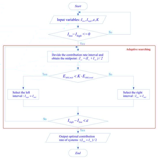
Figure 3.
Adaptive searching process of optimal contribution rate.
The verification that the system can identify the optimal contribution sample set automatically via the above-mentioned four steps will be demonstrated in the next section.
4. The Polydisperse Drag Model
4.1. Drag Model without OCRA
The learning process of the ANN can be regarded as the process of finding the optimal solution in the given error tolerance of the system. The better compatibility and self-learning capabilities of ANN, which are different from traditional regression methods, are promising to obtain the implicit connections and relationships among variables under different granular sizes. Because the difference of granular size will bring obvious heterogeneity in the granular flow, the drag force model of a polydisperse system has complex and implicit nonlinear characteristics. Generally, it has great advantages for the application of ANN to establish the polydisperse drag model.
Since a small training sample set will produce large deviations for ANN training, it is not reasonable to use a small training sample set in the training process. Meanwhile, the training sample set should not be set too large either, considering the computational efficiency and over-fitting problems. In order to find a reasonable training sample set, we start with 990 samples and increase samples with the interval size of and to search for the optimal number of training samples in each interval (, ). The specific searching process and results are illustrated in Appendix B.
After preprocessing the training sample set, a single hidden layer with a 15-neuron BP neural network is used to fit the training data. The LM algorithm and Tanh function are used as the learning method and activation function, respectively, in addition to the input and output variables, which are shown in Figure 2. Since the prediction results are similar, we only show the drag force of granules of different sizes when .
Figure 4 presents the neural network; in general, it can accurately describe the drag force of the polydisperse granular system. Yet, it can still be shown that there is an accuracy difference in the prediction of different-sized granules. From the prediction results, ANN has good prediction accuracy for larger-sized granules (see in Figure 4c,d), but it produces certain deviations for smaller granules, and these deviations will become more obvious in a larger Reynolds number flow system. The main reason is perhaps that the motion of smaller granules is prone to be influenced by larger granules in polydisperse granular flow, and it will lead to irregular features for a smaller granule’s motion that will bring drastic fluctuations in the granular drag force. Furthermore, some smaller granules that are distributed with larger ones will result in heterogeneous distributions. This distribution will cause drastic complex nonlinear relationships in the drag force distribution. Thus, the complicated non-smooth functional relationship between drag force and other variables will appear. On the other hand, the ANN model can achieve more accurate predictions for smooth and flat functional relationships, whereas when ANN encounters the input and output fitting samples with complicated non-smooth functional relationships, it may produce a certain deviation, and this deviation becomes larger as the complex functional relationship becomes stronger. Thus, there will be certain deviations in the prediction of the drag force for smaller granules. Toward these deviations, it is difficult to eliminate them by only considering commonly used inputs in computation, including the mathematical expectations and variance of granular diameters. Thus, it is worth conducting more in-depth studies in searching for the more efficient inputs of ANN in future work.
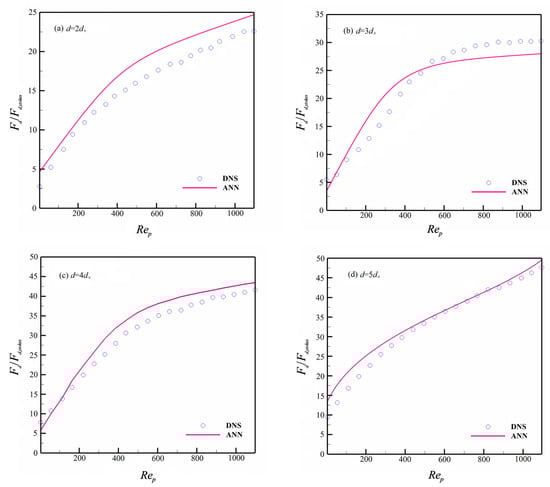
Figure 4.
Dimensionless drag force prediction without OCRA.
4.2. Adaptive Advantages of OCRA
To verify that the OCRA can find the most valuable training samples adaptively under the given number of samples, we first randomly select 1000, 1300, and 1600 samples without OCRA for ANN training. These samples are named random training samples, and then 1000 training samples by using the OCRA, which are named adaptive training samples, are employed to train the ANN. The conditions of the numerical experiment are the same as in Section 4.1. The prediction accuracy and CPU time of different training samples in ANN prediction for are demonstrated in Figure 5 and Table 7.
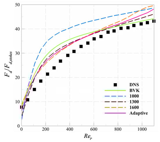
Figure 5.
Different training samples in ANN prediction.
Table 7.
CPU time for different number of training samples.
As shown in Figure 5, the training error of ANN at decreases obviously when the number of training samples increases from 1000 to 1300. However, when the training samples increase from 1300 to 1600, the prediction error of the ANN drag model decreases a little. It can be concluded that the effective samples account for a large proportion in the training samples from 1000 to 1300, so it makes the training error of ANN decrease rapidly. However, in the training samples from 1300 to 1600, the ineffective samples, which are redundant and singular samples, account for the mainstream; these samples have no obvious effect on the improvement of the training accuracy and even reduce the training accuracy of the ANN. The results demonstrate that a large original training sample set will inevitably have some redundant and singular samples, and these “unusual samples” will cause repeat training and even over-fitting problems of the ANN in a certain prediction zone. It still can be inferred from Figure 5 that the prediction accuracy of 1000 samples by using the OCRA is close to that of 1300 random samples, which is much higher than the accuracy of 1000 random samples. Yet, the CPU consumed time for ANN training by 1000 adaptive samples, as shown in Table 7, is 21% less than that of 1300 random training samples. The conclusion can be drawn that the OCRA can find the most valuable training samples for the improvement of training efficiency in the ANN drag model. Simultaneously, a certain number of low-contribution-rate training samples are excluded by this adaptive algorithm. As a matter of fact, the computational efficiency of the ANN drag model can be improved obviously. In general, the OCRA is an effective tool to exclude the redundant and singular samples in ANN training.
4.3. Drag Model with OCRA
So far, we have established an ANN drag model of a polydisperse granular system in Section 4.1. In order to verify the feasibility of OCRA in the ANN drag model, the ANN drag model with OCRA will be established, and its predicted results will be analyzed in this section.
First, the prediction accuracy of ANN with the OCRA needs to be explored. We use 1290 random training samples and 1000 adaptive training samples to train the ANN and ANN with OCRA, respectively. Then, the two drag models will be employed to predict the dimensionless drag force of a polydisperse granular system. The experimental conditions are the same as in Section 4.1, and the weight matrices and biases from the input layer to the hidden layer and the hidden layer to the output layer of the trained neural network are illustrated in Appendix C.
After comparisons of the predicted results in a different void fraction of the granular system, the results demonstrated that in a relatively dilute granular system, the ANN with OCRA outperforms the ANN in the situation with a wide range of granular sizes. The representative predicted results of the granular system, which are , are demonstrated in Figure 6. In a relatively dense granular system, ANN with OCRA and ANN have a similar prediction accuracy in general (see Table 8); both have their own advantages. Figure 7 shows the drag force predictions of the granular system when .
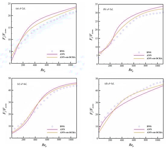
Figure 6.
Dimensionless drag force prediction when .
Table 8.
The MRE of two models in predicting different size of granules.
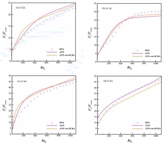
Figure 7.
Dimensionless drag force prediction when .
As shown in Figure 7, when ANN and ANN with OCRA predict the drag force of medium-sized granules in , the overall prediction capability of the two drag models are approximately the same. Specifically, considering the granule size of , the prediction accuracy of ANN with OCRA is slightly better than ANN. For the granule size of , ANN with OCRA and ANN have a similar prediction accuracy in general. However, in smaller and larger granules (, ) ANN gives better results than the ANN with OCRA drag model. Generally, the prediction accuracy of ANN with OCRA is better than ANN in the polydisperse granular system. The results show that, although a certain portion of samples is excluded in the ANN with OCRA model, the prediction accuracy still increases. It can be inferred that OCRA plays an active role in preventing over-fitting problems and repeated ineffective training for the ANN drag model. Meanwhile, compared to the DNS results, ANN with OCRA has more prediction deviations than ANN for the granular size and generally (see Figure 7). The reason may be that, due to the filtering of OCRA, the information loss of larger and smaller granules in the training process will produce a certain prediction deviation. However, the loss of information for medium-sized granules in the ANN with OCRA training does not significantly affect the predicted results, which is probably because the large number of granules will lead to the information loss of medium-sized granules easily compensated for by other similar medium-sized granules. On the other hand, the smaller and larger granules have difficulty achieving this compensation because of their smaller amount, and this phenomenon will become worse in denser granular systems that are dominated by the heterogeneous configuration of a granular cluster. Nevertheless, considering that such a large part of the flow in nature is relatively dilute flow, ANN with OCRA can be a suitable tool to capture the characteristics of flow in nature.
Next, it is needed to explore the efficiency improvement of the OCRA in establishing the ANN drag model. We use the training error of 1290 samples as the standard error (MSE of 1290 samples) to find the training set of the optimal contribution rate of the system with the given error tolerance, i.e.,, and the OCRA is used in searching the most valuable samples. The specific searching processes are recorded below in Table 9.
Table 9.
The searching process of OCRA.
Table 9 shows the OCRA has found the optimal contribution rate of the system in the given error tolerance , which is found to be 0.9140625, and the optimal training set has 1052 samples through 7 steps to find these samples. The optimal contribution sample set, which only accounts for 82% of the original data volume, provides a 91.4% contribution, and the system’s computing efficiency is obviously improved. It still can be concluded that using the OCRA to train the ANN drag model can effectively reduce the amount of training samples without significantly increasing the system errors, and the computational efficiency of the ANN drag model will be improved.
4.4. Drag Model Validation
To verify the validity of the ANN with OCRA drag model in the polydisperse system, we compare the prediction results of ANN that used OCRA with the well-known BVK formula [27], Cello et al. formula [21], and HS formula [30] in polydisperse and monodisperse systems. The empirical formula and prediction results are shown in Table 10 and Figure 8 and Figure 9.
Table 10.
Empirical drag formulas for comparison.
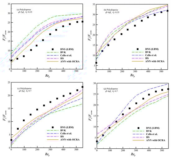
Figure 8.
Predictions of different drag models in polydisperse system [21,27,30].
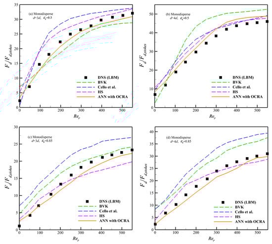
Figure 9.
Predictions of different drag models in monodisperse system [21,27,30].
As shown in Figure 8a,b, when we explore the drag force prediction of in the polydisperse system, the ANN with OCRA model achieves the best predicted accuracy for medium-sized granules () compared to the Cello et al. and HS formulas. The BVK formula suffers the lowest accuracy of all four drag models. For the larger-sized granules (), Cello et al.’s formula shows the best performance among the 4 drag models; especially, these advantages will become more obvious when . On the other hand, the ANN with OCRA has the lowest predicted accuracy compared to the HS and BVK drag models. However, when the 4 drag models were considered in a polydisperse diluted granular system (), the accuracy of the ANN with OCRA drag model is better than the drag model by HS, Cello et al., and BVK in general. In addition, when we explore the drag prediction of these models in a monodisperse granular system (see Figure 9 and Table 11), the accuracy of ANN with OCRA is better than the BVK and HS drag models in terms of medium-sized granules () with void fractions and ; the Cello et al. drag model has the lowest predicted accuracy. Similar results are shown in the granules () of a monodisperse granular system; ANN with OCRA has the best prediction accuracy, followed by the HS drag model, and the BVK and Cello et al. drag models have the lowest prediction accuracy for granules () in and , respectively.
Table 11.
MRE of each drag model in Figure 9.
The simulation results demonstrate that ANN with OCRA has both advantages and disadvantages in different physical conditions. For the advantages, to start with, the ANN with OCRA drag model has obvious advantages in predicting the drag force of medium-sized granules in the polydisperse granular system compared to the other three analytic drag formulas. Next, ANN with OCRA performs well in predicting the larger-sized granules in a relatively dilute polydisperse granular system. Finally, the performance of ANN with OCRA is generally satisfied with the predicting results in a monodisperse granular system. For the disadvantages, ANN with OCRA does not achieve the ideal predicted results in the relatively dense granular system for larger granules. Taking into account this, it is advised to adopt Cello et al.’s drag model for prediction. Therefore, it can be concluded that the ANN with OCRA drag model is good at the prediction of polydisperse granules with a relatively wide concentration and has better compatibility in a monodisperse granular system. There may be three reasons that we have inferred. First, due to the analytic formula, which the other three formulas hold, having a fixed structure, a fixed functional structure has difficulty accurately describing the characteristics of two different flow systems indeed. Second, the ANN has the advantages of self-learning ability and adequate compatibility. The drag force model based on ANN might be easier for switching accurately between monodisperse and polydisperse systems. Third, the OCRA can remove some redundant and singular samples in the training sample set, which can reduce the probability of over-fitting problems in the ANN sample fitting. Therefore, under the accepted tolerance of system errors, the ANN with OCRA drag model has a wide range of applicability in the polydisperse granular system and can also be compatible with monodisperse systems. All in all, considering the performance of each drag model, the ANN with OCRA is suggested to be applied in the prediction of a relatively dilute granular system and a dense granular system for medium-sized granules; Cello et al.’s drag model is suggested to be adopted in the relatively dense granular system for larger granules. The HS drag model is more applicable in a monodisperse granular system.
5. Conclusions
A reasonable ANN model has been successfully established for describing the drag force in polydisperse granular flows. To accomplish this task, the 3D LBM for a polydisperse granular system is used to obtain diverse training data, and then the structures of ANN, including the network layer, learning algorithm, neurons of hidden layers, activation function, and input variables, were comprehensively discussed regarding the computational efficiency and Spearman correlation coefficient between the outputs and expected ones. For the training of ANN, a new adaptive algorithm for a polydisperse drag model was proposed to improve the training efficiency and avoid the over-fitting problem, where redundant and singular samples can be automatically eliminated from the training set. By comparing and analyzing the simulation results, the ANN drag model has good prediction ability in the range of , , , and . Finally, there are several conclusions that we have obtained.
- (a)
- A single-hidden-layer BP neural network with 4 input neurons and 15 hidden neurons, with the activation function of Tanh and the network established by the LM learning method, can effectively realize complex nonlinear mapping in a polydisperse drag model.
- (b)
- Using the OCRA to train the ANN drag model can effectively improve the computational efficiency of ANN, which does not significantly increase the system errors.
- (c)
- Due to ANN having advantages of self-learning ability and good compatibility, the drag model based on ANN can realize the good prediction of both the polydisperse and monodisperse granular systems.
- (d)
- The proposed kernel function based on the exponential form can process training samples of polydisperse drag force effectively for the contribution rate analysis.
In brief, ANN has obvious advantages in the construction of the drag model of the polydisperse granular system, considering the complex non-linear relationship between the variables. The verified structure of the ANN drag model can effectively realize the drag prediction both in monodisperse and polydisperse granular systems. Moreover, using the OCRA to train the ANN drag model can obviously improve the computational efficiency without significantly increasing the system errors. Nevertheless, the prediction accuracy of ANN with OCRA for the larger granules in a relatively dense system still needs to be improved; in light of these imperfections, a more novel structure and efficient training strategy for the ANN drag model can be taken into consideration in future works.
Author Contributions
Conceptualization, X.L. and X.W.; methodology, X.W. and J.O.; software, J.O. and J.D.; formal analysis, X.L. and X.W.; writing—original draft preparation, X.L.; writing—review and editing, X.W. and J.O.; funding acquisition, X.W. and J.O. All authors have read and agreed to the published version of the manuscript.
Funding
This research was funded by the National Natural Science Foundation of China (Grant No. 11971387) and the Fundamental Research Funds for the Central Universities (Grant No. D5000230061).
Institutional Review Board Statement
Not applicable.
Informed Consent Statement
Not applicable.
Data Availability Statement
Data will be available upon a reasonable request.
Acknowledgments
The authors would like to thank the anonymous referees, whose valuable comments helped to improve this paper. The authors extend their gratitude to Hussein A. H. Muhammed for his careful checking and improving of the language expression of the manuscript.
Conflicts of Interest
The authors declare no conflict of interest.
Appendix A
The Impact of Input and Output Correlation
To construct a nonlinear mapping between the inputs and the expected outputs by using the ANN, it is necessary to discuss the correlation between different input and output variables. Taking the particle Reyolds number given in Formula (8) as an example, is a function of the solid volume fraction and the slip velocity . Table A1 lists the relationship between input and output variables of the ANN.
Table A1.
The relationship between input and output variables.
Table A1.
The relationship between input and output variables.
| Combination | Input | Output |
|---|---|---|
| A | , , | |
| B | , , , |
Table A2 shows the Spearman correlation coefficients between the outputs and the expected outputs (results of DNS) for four independent experiments. The results show that the combination A is much more efficient than the combination B.
Table A2.
Spearman correlation coefficient in four independent experiments.
Table A2.
Spearman correlation coefficient in four independent experiments.
| Exp. | Combination A | Combination B |
|---|---|---|
| 1 | 0.9801 | 0.6793 |
| 2 | 0.9807 | 0.7009 |
| 3 | 0.9873 | 0.6935 |
| 4 | 0.9896 | 0.7128 |
| 0.9844 | 0.6966 |
Appendix B
The Searching Process of Optimal Number of Training Samples
To find a reasonable training sample set, we start with 990 samples and increase samples with the same step size. The , , , and CPU time of the trained ANN are given in Table A3 as the value of and . , , and denote the average MSE, MAE, and MRE of all size granules, respectively. The CPU time is the summation of the training and prediction times consumed by the ANN when the error limit is set by .
Table A3.
The error and calculation time increase with the number of samples.
Table A3.
The error and calculation time increase with the number of samples.
| Training Samples | CPU Time (s) | |||
|---|---|---|---|---|
| 990 | 0.6369 | 0.9315 | 0.0782 | 203.2 |
| 1050 | 0.5421 | 0.8113 | 0.0509 | 211.3 |
| 1110 | 0.4659 | 0.7815 | 0.0397 | 227.6 |
| 1170 | 0.4237 | 0.7425 | 0.0335 | 242.2 |
| 1230 | 0.3542 | 0.7101 | 0.0291 | 261.9 |
| 1290 | 0.2955 | 0.6879 | 0.0091 | 278.5 |
| 1350 | 0.2925 | 0.6821 | 0.0089 | 315.9 |
| 1410 | 0.2913 | 0.6801 | 0.0086 | 382.6 |
| 1470 | 0.2901 | 0.6779 | 0.0085 | 497.2 |

Figure A1.
The relationship between training error and sample size [33].
Figure A1.
The relationship between training error and sample size [33].

As shown in Table A3, when the number of training samples increases from 990, the training errors , and of the system decrease gradually. When the number of training samples approaches 1290, the reduction speed of the training error gradually slackens, but the consumed CPU time increases rapidly. Considering the computational efficiency of the system and similar results in other intervals, 1290 training samples are adopted as the training dataset in each interval.
Appendix C
Table A4.
ANN simulation parameters [61].
Table A4.
ANN simulation parameters [61].
| Structure | Parameters |
|---|---|
| Input variables | , , , |
| Output variables | |
| Hidden layer | 1 |
| Learning algorithm | Levenberg–Marquardt |
| Activation function | Tanh |
| Number of neurons in hidden layer | 15 |
| ANN mode | Back propagation ANN |
Weights and biases matrices when ANN training is complete.
References
- Bilal, M.; Ullah, I.; Alam, M.M.; Weera, W.; Galal, A.M. Numerical simulations through PCM for the dynamics of thermal enhancement in ternary MHD hybrid nanofluid flow over plane sheet, cone, and wedge. Symmetry 2022, 14, 2419. [Google Scholar] [CrossRef]
- Bilal, M.; Ullah, I.; Alam, M.M.; Shah, S.I.; Eldin, S.M. Energy transfer in Carreau Yasuda liquid influenced by engine oil with magnetic dipole using tri-hybrid nanoparticles. Sci. Rep.-UK 2023, 13, 5432. [Google Scholar] [CrossRef] [PubMed]
- Bilal, M.; Ali, A.; Hejazi, H.A.; Mahmuod, S.R. Numerical study of an electrically conducting hybrid nanofluid over a linearly extended sheet. Z. Angew Math. Mech. 2023, 103, e202200227. [Google Scholar] [CrossRef]
- Alqahtani, A.M.; Bilal, M.; Ali, A.; Alsenani, T.R.; Eldin, S.M. Numerical solution of an electrically conducting spinning flow of hybrid nanofluid comprised of silver and gold nanoparticles across two parallel surfaces. Sci. Rep.-UK 2023, 13, 7180. [Google Scholar] [CrossRef] [PubMed]
- Elsebaee, F.A.A.; Bilal, M.; Mahmoud, S.R.; Balubaid, M.; Shuaib, M.; Asamoah, J.K.K.; Ali, A. Motile micro-organism based trihybrid nanofluid flow with an application of magnetic effect across a slender stretching sheet: Numerical approach. AIP Adv. 2023, 13, 035237. [Google Scholar] [CrossRef]
- Ullah, I. Heat transfer enhancement in Marangoni convection and nonlinear radiative flow of gasoline oil conveying Boehmite alumina and aluminum alloy nanoparticles. Int. Commun. Heat Mass 2022, 132, 105920. [Google Scholar] [CrossRef]
- Hayat, T.; Ullah, I.; Muhammad, T.; Alsaedi, A. Magnetohydrodynamic (MHD) three-dimensional flow of second grade nanofluid by a convectively heated exponentially stretching surface. J. Mol. Liq. 2016, 220, 1004–1012. [Google Scholar] [CrossRef]
- Wang, L.M.; Wu, C.Y.; Ge, W. Effect of particle clusters on mass transfer between gas and particles in gas-solid flows. Powder. Technol. 2017, 319, 221–227. [Google Scholar] [CrossRef]
- Liu, X.W.; Ge, W.; Wang, L.M. Scale and structure dependent drag in gas–solid flows. AIChE J. 2020, 66, e16883. [Google Scholar] [CrossRef]
- Alchikh-Sulaiman, B.; Alian, M.; Ein-Mozaffari, F.; Lohi, A.; Upreti, S.R. Using the discrete element method to assess the mixing of polydisperse solid particles in a rotary drum. Particuology 2016, 25, 133–142. [Google Scholar] [CrossRef]
- Zhang, Y.; Zhao, Y.M.; Lu, L.Q.; Ge, W.; Wang, J.W.; Duan, C.L. Assessment of polydisperse drag models for the size segregation in a bubbling fluidized bed using discrete particle method. Chem. Eng. Sci. 2017, 160, 106–112. [Google Scholar] [CrossRef]
- Karzar-Jeddi, M.; Luo, H.; Cummings, P.T. Mobilities of polydisperse hard spheres near a no-slip wall. Comput. Fluids. 2018, 176, 40–50. [Google Scholar] [CrossRef]
- Wang, Y.; Ouyang, J.; Wang, X.D. Machine learning of lubrication correction based on GPR for the coupled DPD–DEM simulation of colloidal suspensions. Soft Matter 2021, 17, 5682–5699. [Google Scholar] [CrossRef] [PubMed]
- Wang, X.D.; Chen, K.; Kang, T.; Ouyang, J. A dynamic coarse grain discrete element method for gas-solid fluidized beds by considering particle-group crushing and polymerization. Appl. Sci. 2020, 10, 1943. [Google Scholar] [CrossRef]
- Knight, C.; O’Sullivan, C.; van Wachem, B.; Dini, D. Computing drag and interactions between fluid and polydisperse particles in saturated granular materials. Comput. Geotech. 2020, 117, 103210. [Google Scholar] [CrossRef]
- Akiki, G.; Jackson, T.L.; Balachandar, S. Pairwise interaction extended point-particle model for a random array of monodisperse spheres. J. Fluid Mech. 2017, 813, 882–928. [Google Scholar] [CrossRef]
- Akiki, G.; Moore, W.C.; Balachandar, S. Pairwise-interaction extended point-particle model for particle-laden flows. J. Comput. Phys. 2017, 351, 329–357. [Google Scholar] [CrossRef]
- Lindberg, C.S.; Manuputty, M.Y.; Yapp, E.K.; Akroyd, J.; Xu, R.; Kraft, M. A detailed particle model for polydisperse aggregate particles. J. Comput. Phys. 2019, 397, 108799. [Google Scholar] [CrossRef]
- Li, J.H. Particle-Fluid Two-Phase Flow: The Energy-Minimization Multi-Scale Method; Metallurgical Industry Press: Beijing, China, 1994. [Google Scholar]
- Li, J.H.; Kwauk, M. Multiscale nature of complex fluid− particle systems. Ind. Eng. Chem. Res. 2001, 40, 4227–4237. [Google Scholar] [CrossRef]
- Cello, F.; Di Renzo, A.; Di Maio, F.P. A semi-empirical model for the drag force and fluid–particle interaction in polydisperse suspensions. Chem. Eng. Sci. 2010, 65, 3128–3139. [Google Scholar] [CrossRef]
- Qin, Z.Y.; Zhou, Q.; Wang, J.W. An EMMS drag model for coarse grid simulation of polydisperse gas–solid flow in circulating fluidized bed risers. Chem. Eng. Sci. 2019, 207, 358–378. [Google Scholar] [CrossRef]
- Li, X.; Ouyang, J.; Wang, X.D.; Chu, P.P. A drag force formula for heterogeneous granular flow systems based on finite average statistical method. Particuology 2021, 55, 94–107. [Google Scholar] [CrossRef]
- van der Hoef, M.A.; Beetstra, R.; Kuipers, J.A.M. Lattice-Boltzmann simulations of low-Reynolds-number flow past mono- and bi-disperse arrays of spheres: Results for the permeability and drag force. J. Fluid Mech. 2005, 528, 233–254. [Google Scholar] [CrossRef]
- Hill, R.J.; Koch, D.L.; Ladd, A.J. The first effects of fluid inertia on flows in ordered and random arrays of spheres. J. Fluid Mech. 2001, 448, 213–241. [Google Scholar] [CrossRef]
- Benyahia, S.; Syamlal, M.; O’Brien, T.J. Extension of Hill–Koch–Ladd drag correlation over all ranges of Reynolds number and solids volume fraction. Powder Technol. 2006, 162, 166–174. [Google Scholar] [CrossRef]
- Beetstra, R.; van der Hoef, M.A.; Kuipers, J.A.M. Drag force of intermediate Reynolds number flow past mono- and bidisperse arrays of spheres. AIChE J. 2007, 53, 489–501. [Google Scholar] [CrossRef]
- Ergun, S.; Orning, A.A. Fluid flow through randomly packed columns and fluidized beds. Ind. Eng. Chem. 1949, 41, 1179–1184. [Google Scholar] [CrossRef]
- Sarkar, S.; van der Hoef, M.A.; Kuipers, J.A.M. Fluid–particle interaction from lattice Boltzmann simulations for flow through polydisperse random arrays of spheres. Chem. Eng. Sci. 2009, 64, 2683–2691. [Google Scholar] [CrossRef]
- Holloway, W.; Sundaresan, S. Filtered models for bidisperse gas–particle flows. Chem. Eng. Sci. 2014, 108, 67–86. [Google Scholar] [CrossRef]
- Yin, X.L.; Sundaresan, S. Fluid-particle drag in low Reynolds number polydisperse gas-solid suspensions. AIChE J. 2009, 55, 1352–1368. [Google Scholar] [CrossRef]
- Rong, L.W.; Dong, K.J.; Yu, A.B. Lattice-Boltzmann simulation of fluid flow through packed beds of uniform spheres: Effect of porosity. Chem. Eng. Sci. 2013, 99, 44–58. [Google Scholar] [CrossRef]
- Jiang, Y.D.; Kolehmainen, J.; Gu, Y.L.; Kevrekidis, Y.G.; Ozel, A.; Sundaresan, S. Neural-network-based filtered drag model for gas-particle flows. Powder Technol. 2019, 346, 403–413. [Google Scholar] [CrossRef]
- He, L.; Tafti, D.K. A supervised machine learning approach for predicting variable drag forces on spherical particles in suspension. Powder Technol. 2019, 345, 379–389. [Google Scholar] [CrossRef]
- Zhu, L.T.; Tang, J.X.; Luo, Z.H. Machine learning to assist filtered two-fluid model development for dense gas-particle flows. AIChE J. 2020, 66, e16973. [Google Scholar] [CrossRef]
- Zhang, Y.; Jiang, M.; Chen, X.; Yu, Y.L.; Zhou, Q. Modeling of the filtered drag force in gas–solid flows via a deep learning approach. Chem. Eng. Sci. 2020, 225, 115835. [Google Scholar] [CrossRef]
- Luo, K.; Wang, D.; Jin, T.; Wang, S.; Wang, Z.; Tan, J.H.; Fan, J.R. Analysis and development of novel data-driven drag models based on direct numerical simulations of fluidized beds. Chem. Eng. Sci. 2021, 231, 116245. [Google Scholar] [CrossRef]
- Tang, Y.L.; Peters, E.; Kuipers, J.A.M. Direct numerical simulations of dynamic gas-solid suspensions. AIChE J. 2016, 62, 1958–1969. [Google Scholar] [CrossRef]
- Ashwin, N.R.; Cao, Z.; Muralidhar, N.; Tafti, D.; Karpatne, A. Deep learning methods for predicting fluid forces in dense particle suspensions. Powder Technol. 2022, 401, 117303. [Google Scholar] [CrossRef]
- Hwang, S.; Pan, J.; Fan, L.S. Deep learning for drag force modelling in dilute, poly-dispersed particle-laden flows with irregular-shaped particles. Chem. Eng. Sci. 2023, 266, 118299. [Google Scholar] [CrossRef]
- Hwang, S.; Pan, J.; Fan, L.-S. A machine learning-based interaction force model for non-spherical and irregular particles in low Reynolds number incompressible flows. Powder Technol. 2021, 392, 632–638. [Google Scholar] [CrossRef]
- Nikolopoulos, A.; Samlis, C.; Zeneli, M.; Nikolopoulos, N.; Karellas, S.; Grammelis, P. Introducing an artificial neural network energy minimization multi-scale drag scheme for fluidized particles. Chem. Eng. Sci. 2021, 229, 116013. [Google Scholar] [CrossRef]
- Kobayashi, W.; Shimura, T.; Mitsuishi, A.; Iwamoto, K.; Murata, A. Prediction of the drag reduction effect of pulsating pipe flow based on machine learning. Int. J. Heat Fluid Flow 2021, 88, 108783. [Google Scholar] [CrossRef]
- Li, C.X.; Singh, N.; Andrews, A.; Olson, B.A.; Schwartzentruber, T.E.; Hogan, J.C.J. Mass, momentum, and energy transfer in supersonic aerosol deposition processes. Int. J. Heat Mass Tran. 2019, 129, 1161–1171. [Google Scholar] [CrossRef]
- Montavon, G.; Orr, G.; Müller, K.R. Neural Networks: Tricks of the Trade; Springer Press: Berlin/Heidelberg, Germany, 2003; pp. 5–79. [Google Scholar]
- Huang, H.; Sukop, M.; Lu, X. Multiphase Lattice Boltzmann Methods: Theory and Application; John Wiley & Sons: Hoboken, NJ, USA, 2015. [Google Scholar]
- Chen, S.; Doolen, G.D. Lattice Boltzmann method for fluid flows. Annu. Rev. Fluid Mech. 1998, 30, 329–364. [Google Scholar] [CrossRef]
- He, X.; Luo, L.S. Lattice Boltzmann model for the incompressible Navier-Stokes equation. J. Stat. Phys. 1997, 88, 927–944. [Google Scholar] [CrossRef]
- He, X.; Luo, L.S. A priori derivation of the lattice Boltzmann equation. Phys. Rev. E 1997, 55, R6333–R6336. [Google Scholar] [CrossRef]
- Chapman, S.; Cowling, T.G. The Mathematical Theory of Non-Uniform Gases, 3rd ed.; Cambridge University Press: Cambridge, UK, 1970. [Google Scholar]
- Chen, Y.; Third, J.R.; Müller, C.R. A drag force correlation for approximately cubic particles constructed from identical spheres. Chem. Eng. Sci. 2015, 123, 146–154. [Google Scholar] [CrossRef]
- Su, J.; Ouyang, J.; Wang, X.D.; Yang, B.X. Lattice Boltzmann method coupled with the Oldroyd-B constitutive model for a viscoelastic fluid. Phys. Rev. E 2013, 88, 053304. [Google Scholar] [CrossRef]
- Ladd, A.J.C.; Verberg, R. Lattice-Boltzmann simulations of particle-fluid suspensions. J. Stat. Phys. 2001, 104, 1191–1251. [Google Scholar] [CrossRef]
- Pacek, A.W.; Man, C.C.; Nienow, A.W. On the Sauter mean diameter and size distributions in turbulent liquid/liquid dispersions in a stirred vessel. Chem. Eng. Sci. 1998, 53, 2005–2011. [Google Scholar] [CrossRef]
- Goodfellow, I.; Bengio, Y.; Courville, A. Deep Learning; MIT Press: Cambridge, MA, USA, 2016; pp. 118–131. [Google Scholar]
- Wu, G.; Ouyang, J.; Li, Q. Revised drag calculation method for coarse grid Lagrangian–Eulerian simulation of gas–solid bubbling fluidized bed. Powder Technol. 2013, 235, 959–967. [Google Scholar] [CrossRef]
- Richard, A.J.; Miller, L.; Freund, J.E. Probability and Statistics for Engineers; Pearson Education Press: London, UK, 2000; pp. 469–481. [Google Scholar]
- Jolliffe, I.T. Principal Component Analysis; Springer: Berlin/Heidelberg, Germany, 2002; pp. 30–59. [Google Scholar]
- Lee, J.M.; Yoo, C.K.; Choi, S.W.; Vanrolleghem, P.A.; Lee, I.B. Nonlinear process monitoring using kernel principal component analysis. Chem. Eng. Sci. 2004, 59, 223–234. [Google Scholar] [CrossRef]
- Axler, S. Linear Algebra Done Right; Springer Science & Business Media: Berlin/Heidelberg, Germany, 1997; pp. 75–94. [Google Scholar]
- Viquerat, J.; Hachem, E. A supervised neural network for drag prediction of arbitrary 2D shapes in laminar flows at low Reynolds number. Comput. Fluids. 2020, 210, 104645. [Google Scholar] [CrossRef]


Disclaimer/Publisher’s Note: The statements, opinions and data contained in all publications are solely those of the individual author(s) and contributor(s) and not of MDPI and/or the editor(s). MDPI and/or the editor(s) disclaim responsibility for any injury to people or property resulting from any ideas, methods, instructions or products referred to in the content. |
© 2023 by the authors. Licensee MDPI, Basel, Switzerland. This article is an open access article distributed under the terms and conditions of the Creative Commons Attribution (CC BY) license (https://creativecommons.org/licenses/by/4.0/).