Unstructured Grid-Based River–Coastal Ocean Circulation Modeling towards a Digital Twin of the Seto Inland Sea

Abstract

As computational techniques advance, the scope of digital twins (DTs) is expanding to encompass entire cities, oceans, or even the Earth. Digital twins of oceans can provide highly comprehensive insights and predictions, thus enabling better-informed decision-making regarding ocean-related activities and management. Here, a numerical model of the Seto Inland Sea (SIS), Japan, was built as a basis to establish a digital twin of the SIS. Spatially varying filtering parameters and grid resolutions were applied to facilitate the robust and accurate simulation of coastal and oceanic processes even under varying extreme conditions. The modeling results were validated using observational datasets from forty-two tidal stations, one mooring system, and thirteen water thermometers. The results represented tidal variations, with NRMSE values below 0.15 and R² values exceeding 0.87 at all tidal stations. The NRMSE and R² values for currents were approximately 0.14 and 0.76, respectively. The model reproduced the extreme storm surge event causing a sea level rise of 1.5 m near Osaka City resulting from Typhoon Jebi in 2018. The model was shown to enable analyses of complex circulations and hazards in the SIS by accurately replicating barotropic and baroclinic processes. After additional modules are added, this model will serve as a basis for constructing a digital twin of the SIS.

1. Introduction

A digital twin (DT) is a relatively emerging technology because its first concept was introduced in 2002 by Michael Grieves [1], mentioning three components of DTs: real space, virtual space, and the data-flow link connecting these spaces. At first, DTs were primarily utilized within the aerospace industry, but its adoption has since spread to other industries, fueled by the growing importance of digital transformation and the emergence of Industry 4.0 [2]. By offering an opportunity to simulate and optimize production systems, DTs can increase manufacturers’ competitiveness, productivity, and efficiency [3].

Previously, it was applied to experiments related to manufacturing, aviation, and healthcare, such as spacecraft, aircraft, automotive, and medical devices [4]. These scales were limited to one craft or one machine, but the scales of DTs became dramatically expanded due to the rapid growth of techniques related to database computation, artificial intelligence, and the Internet of Things (IoT). Currently, efforts to create relatively large-scale DT systems are being implemented to build digital twins of cities, oceans, or even the entire Earth [5].

With this fast-growing field, we should be careful in using terminology about DT because it is used confusingly with digital model and digital shadow [6,7]. These three concepts are mainly distinguished by levels of interaction with the physical system. In cases of ocean models, if we set a model for pre-existing ocean environments using past data, this is just a digital model without any automatic data exchanges with the real world. Further, if the model can automatically receive and consider the observed data, such as meteorological or oceanic data from installed sensors, it is called a digital shadow.

To be a DT, interaction between reality and the model is required. However, it is not easy to affect or test the real marine environment directly on short timescales using a hydrodynamic model due to the vast scale of the real ocean. Therefore, ocean DTs must focus on evaluating the effects of new policies or changing environments by providing a better understanding and predictions of the best-informed decisions. To achieve this purpose, we must prepare a set of interoperable techniques [8], such as qualified datasets, smart visualization platforms, and appropriate analysis tools [9].

The European Centre for Medium-Range Weather Forecasts (ECMWF) developed the Destination Earth (DestinE) project to provide assessments and forecasts of environmental extremes to support risk assessment and management [5]. Facing unprecedented global environmental challenges, such as food, energy, and ecosystem sustainability, the important paradigm of digital ecosystems (DEs) is suggested to be converting all aspects of our life into quantified data, taking an example from DestinE [9]. The Japan Agency for Marine-Earth Science and Technology (JAMSTEC) is developing a high-resolution ocean model as a component of the Four-Dimensional Virtual Earth (4DVE) project in which digital twins of Earth are created.

To support the visualization and analysis of existing datasets, web-based applications have been developed. For instance, MyOceanViewer from Copernicus Marine Service allows users to explore global ocean variables from hindcasts, observations, and forecasts over time and at various depths. A platform integrating available data sources, such as the Copernicus Marine Environment Monitoring Service, Copernicus Land Monitoring Service, and WorldPop, was developed to combine 60 geospatial layers from different sources focusing on the Italian coasts [10].

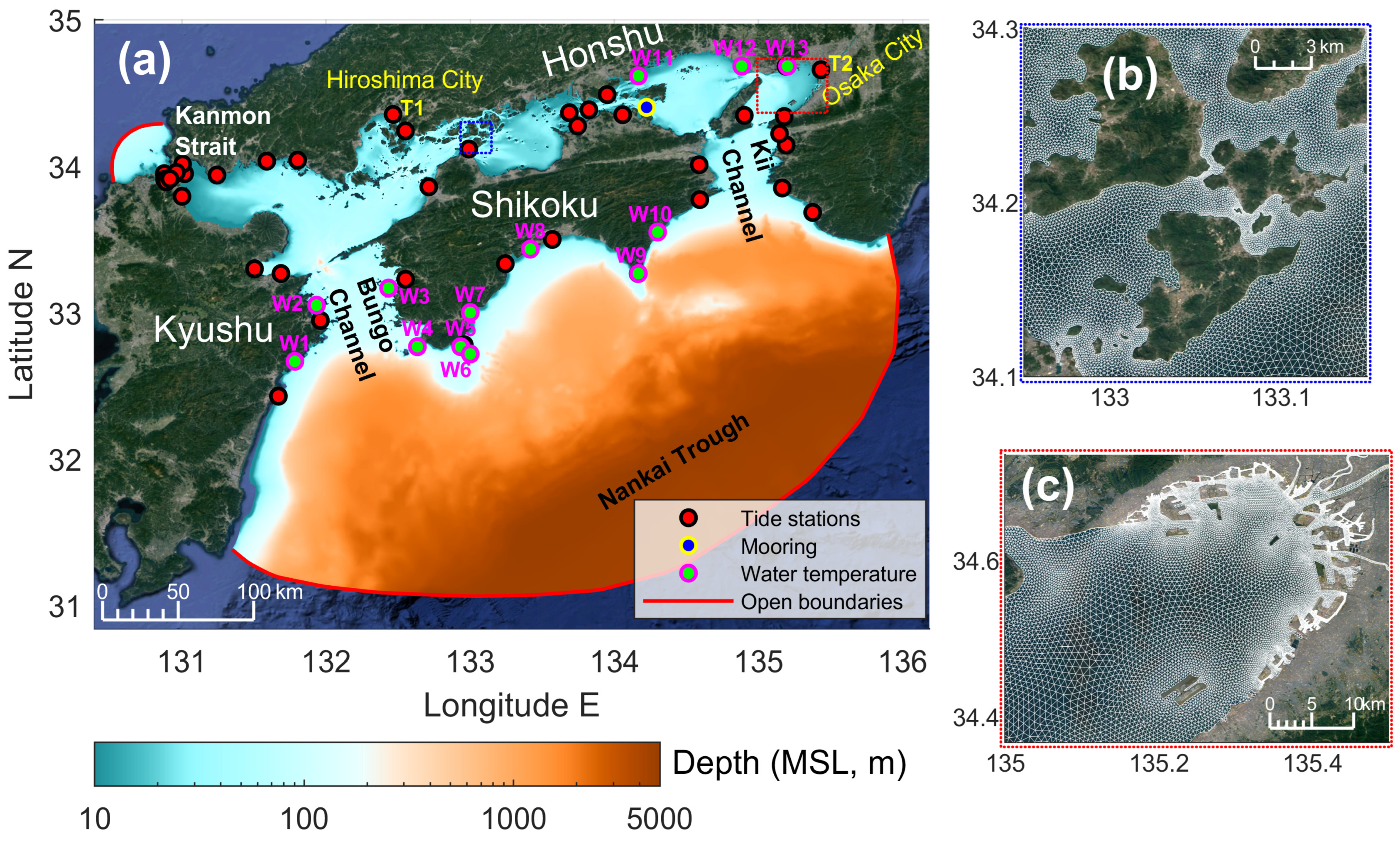
This study will be the cornerstone for establishing a DT system for the Seto Inland Sea (SIS). The SIS is a semi-enclosed coastal sea with an area of approximately 23,000 km², a length of approximately 450 km, and an average depth of approximately 38 m; the SIS is located in the western part of Japan [11]. It has only two connections to the Pacific Ocean through the Bungo and Kii channels and one connection to the East/Japan Sea through the Kanmon Strait. The SIS consists of approximately 700 islands and many narrow straits connecting basins and bays, including Hiroshima Bay and Osaka Bay [11] (Figure 1).

The Semi-implicit Cross-scale Hydroscience Integrated System Model (SCHISM) can be set up to perform efficient and accurate simulations at varying scales, such as creek, lake, river, estuary, shelf, and ocean scales [12,13,14]. The seamless cross-scale modeling system was validated in a global simulation [15]. They showed that a single mesh spanning resolutions from 10 km to 8 m can depict the global ocean, covering a range of scales from the entire extent of the five oceans down to the scale of an estuary. Furthermore, this model supports fluent modules applicable to diverse areas such as tsunami hazards, storm surges, sediment transport, biogeochemistry, water quality, and oil spills. The adoption of an unstructured grid allows users to describe complex coastlines more precisely and the grid can be applied to the other modules as-is.

In this study, we built an unstructured grid-based high-resolution hydrodynamic model of the SIS using SCHISM. The model was established to simulate coastal and oceanic processes, including any extreme weather and events, as robustly and accurately as possible by applying spatially varying filtering parameters depending on possible numerical instability factors and a spatially varying grid resolution depending on the bathymetric gradient to reduce pressure gradient errors. We validated the model results with observational data and visualized the results in a three-dimensional domain. Then, the calibrated model was applied to the extreme storm surge in Osaka Bay that was induced by Typhoon Jebi in 2018.

In the following text, the characteristics of the model and the parameter-setting process are described in Section 2. Section 3 illustrates the validations of the numerical model for tides, temperatures, and currents in the SIS. The storm surge application of the model is described in Section 4. Section 5 shows the 3D visualization and modeling system plan for obtaining a digital twin of the SIS. Conclusions are provided in Section 6.

2. Materials and Methods

2.1. The Seto Inland Sea

The Seto Inland Sea has distinct characteristics that are worthy of studying with the aim of developing a digital twin of the SIS. The first is its location. The SIS is threatened by rainfall-induced flood events [16], typhoon-induced storm surges [17,18] and earthquake-induced tsunamis [11,19]. Additionally, Kuroshio currents pass in front of the SIS in the Pacific. The effect of the convergence of these diverse natural phenomena should be investigated in-depth to prepare for and prevent possible risk factors.

The second notable characteristic is its complexity. The SIS contains an archipelago with two main channels connecting it to the Pacific Ocean. Through narrow and complex straits, tidal waves flowing in from these channels converge near Hiuchi Nada and Bisan Seto in the central part of the SIS. This results in difficulties in reproducing tides in the SIS [20], and although tides were reproduced in a previous study, a quite large root-mean square error (RMSE) of 40 cm was calculated in the inner part of the SIS [21]. Understanding the spatial distributions of currents in these areas is critical for environmental impact assessments, ocean energy resource assessments, marine safety, navigation, sedimentation, aquaculture, and other factors.

The third characteristic is its geographical isolation. The shape of the SIS is an ellipse with a major (minor) axis of approximately 450 km (75 km). However, the widths of its entry channels are 40 km (Bungo and Kii), and the width of the Kanmon strait is 1.5 km. Therefore, the governing characteristics of the volume of the SIS are determined by a few conditions: the boundary conditions of the narrow entrance, freshwater discharged from rivers, and atmospheric conditions in combination with the geographic, topographic/bathymetric and geometric features of the SIS. This means that once an SIS modeling system is established successfully, the quasi-isolated system will be more efficiently manageable, and any scenario cases will be effectively testable by controlling the limiting conditions.

2.2. Framework: SCHISM

We utilized the latest version (v5.9.0) of the Semi-implicit Cross-scale Hydroscience Integrated System Model (SCHISM) [22], a derivative product based on the original SELFE model (v3.1dc) [23]. The Navier–Stokes equations in the hydrostatic form are solved using the semi-implicit finite-element/-volume method, allowing stable simulations. Due to its location within the typhoon belt, the SIS is highly susceptible to extreme weather conditions, such as massive freshwater influxes, strong winds, and high waves caused by typhoons. Therefore, the high stability of SCHISM allows simulations performed in the SIS to be maintained relatively robustly.

The fundamental equations within the hydrodynamic model, SCHISM, are the continuity equation, the momentum equation, and the transport equation, expressed in sequence as follows:

$$\nabla ·\mathbf{u}+\frac{\partial w}{\partial z}=0$$

(1)

$$\frac{D\mathbf{u}}{Dt}=\frac{\partial }{\partial z}\left(\nu \frac{\partial \mathbf{u}}{\partial z}\right)-g\nabla \eta +\mathit{F}$$

(2)

$$\frac{DC}{Dt}=\frac{\partial }{\partial z}\left(\kappa \frac{\partial C}{\partial z}\right)+F_h+Q$$

(3)

where $\mathbf{u}$ is the horizontal velocity with Cartesian components (u, v), $w$ is the vertical velocity, $h$ is the bathymetry, $\eta$ is the free surface elevation, $g$ is the acceleration of gravity (m s⁻²), $C$ is the concentration of tracers, such as salinity and temperature, ν is the vertical eddy viscosity (m² s⁻¹), $\kappa$ is the vertical eddy diffusivity of tracers (m² s⁻¹), $\mathit{F}$ is a momentum forcing, such as the air pressure, Coriolis effect, or horizontal viscosity, $F_h$ is the horizontal diffusion, and $Q$ is the source/sink term for the mass of tracers.

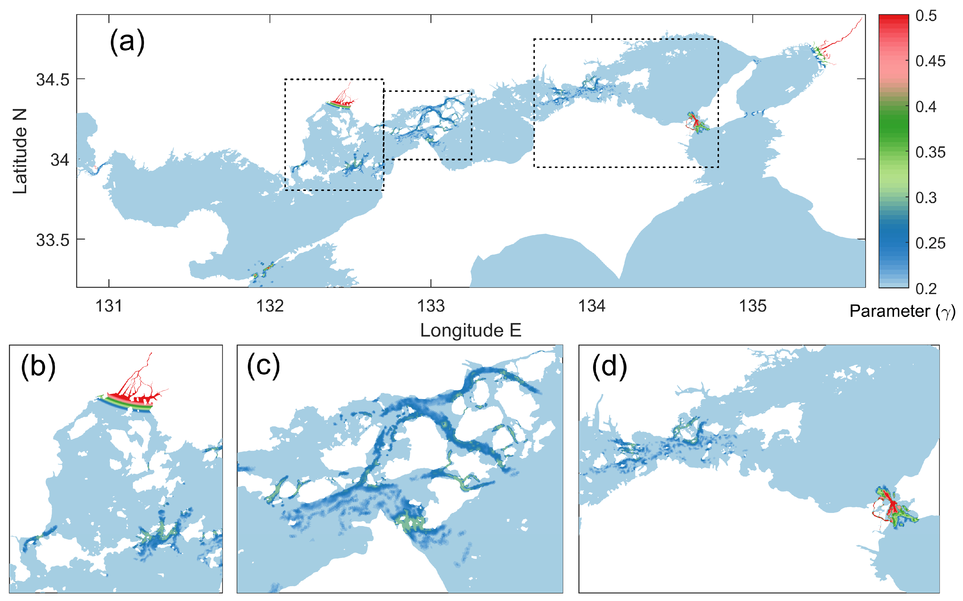
Advection and viscosity schemes in SCHISM include several options, such as the Laplacian viscosity, biharmonic viscosity, and 5-point Shapiro filter, for enhancing momentum stabilization. Without these tools, inertial spurious modes of velocities or temperature can develop during the simulations. Each option demands a diffusion-number-like dimensionless parameter that can be controlled depending on the instability of the model runs. Here, we adopted the 5-point Shapiro filter [24], the application of which can be controlled by a parameter (γ) ranging in value from 0 to 0.5 as follows:

$$\widetilde{u_0}=u_0+\frac{\mathsf{\gamma }}{4}\left(u_1+u_2+u_3+u_4+-4u_0\right)$$

(4)

where $u_0$ is the velocity at side ‘0’ between two elements (here, triangular) and $u_n$ (n = 1, 2, 3, 4) is the velocity at the other two sides of the triangle (2 × 2 = 4). We provide node-specified parameters that vary spatially depending on the possible instability of each node (the maximum current, mesh resolution, and heavy river discharge), as is further explained in the following model setup section.

2.3. Model Setup

The model was simulated for 39 days, from 1 September to 9 October in 2011; this period included the typhoon season and was chosen for the sake of constructing a robust model during extreme atmospheric conditions. The time step for the model was set to 80 s, while the outputs were stored every 12 min. All information about time stated in this paper is based on the local time, Japan Standard Time (JST).

The maximum resolution of the horizontal grid was approximately 30 m around Hiroshima Bay, one of the main study areas of the model. The spatial grid resolution of the model varied flexibly to describe all islands and straits in the SIS (Figure 1b) as long as the number of nodes and cells maintained a reasonable level in terms of the computation time. For Hiroshima City and Osaka City, the complex coastlines with coastal infrastructures were described in great detail (Figure 1c). The maximum size of the mesh was approximately 9800 m near the main open boundary in the Pacific. The resolution of the grid near the Nankai Trough was determined by considering the gradient of bathymetry, as shown in Figure A1, to reduce the pressure gradient force errors in terrain-following (σ) coordinates by describing the steep bathymetric gradients near troughs in great detail. Thus, the total number of nodes and cells became 210,505 and 390,461, respectively, covering the domain with lengths of 500 km × 420 km. Thirty sigma levels were used for the vertical grid. As a result, in terms of the computation time, it took approximately 30 min of real time to simulate one day of model time with ninety-six CPUs. The short simulation time will allow us to apply the near real-time feedback system between reality (physical space) and the model (virtual space).

The Shapiro filter was adopted to suppress spurious velocity or temperature modes by increasing the stability of the model during the simulations. However, the momentum of fluids can be excessively dissipated if a meaninglessly high filter parameter is set, resulting in the unrealistic depression of surface elevations and velocities (the maximum filter value allowed by the model developer is 0.5). The horizontal resolution of our model was high, focusing on the target areas, river mouths, and narrow channels, as explained above. A small uniform value for the parameter such as 0.2 could not prevent the occurrence of spurious modes, resulting in unrealistic velocity patterns along the unstable mesh areas. When the value of 0.5 was applied uniformly, the spurious modes were successfully suppressed, but the momentum that should have been calculated was also suppressed. Applying the parameter uniformly across the entire model domain could not solve this problem. Therefore, we tried to generate a spatially varying parameter field considering instability factors, such as the maximum velocity, mesh resolution, and heavy river discharge, at each node. To obtain the maximum velocity field, we simulated the model with fewer vertical layers than the thirty layers used in this study. Then, the relatively high filter parameter values were calculated at the nodes with high velocities and high resolutions. Additionally, we set relatively high values for the river areas with freshwater discharges. Finally, we created a field for the parameter γ (Figure 2), after which the model simulation could perform much more stably and accurately without spurious modes or excessive energy dissipation.

Careful attention was also paid to creating high-resolution bathymetric information for the numerical simulations. As the base bathymetry data, electronic charts of the M7000 series from the Japan Hydrographic Association were used. This dataset is based on bathymetric contours. It has strengths, especially near narrow and steep sea areas, because the contour intervals are more finely subdivided near these areas. However, the contour interval of the M7000 series is sometimes quite coarse in coastal areas, especially near Osaka Bay. In addition, these bathymetry data do not cover the furthest area of the model. The JODC bathymetry data (at 50, 150, and 500 m resolutions) were therefore replaced and combined for these areas.

The model grid considered in this research comprises the river mouths of the Ota River in Hiroshima Bay and the Yodo River in Osaka Bay, near which hydrographic charts cannot describe the sea depth. To generate bathymetric information for these river-mouth areas, we utilized the heights of watermarks at water level gauges in each river. These heights were measured from an elevation of zero and were provided by the Disaster Prevention Information for Rivers (www.river.go.jp (accessed on 31 May 2022)) of the Ministry of Land, Infrastructure, Transport and Tourism (MLIT). The heights of gauges distributed along the river were interpolated to the grid by assuming linear depth changes between gauges. All the bathymetry data used herein were adjusted in reference to the MSL. The minimum depth was restricted to 3 m due to the present stability of the model.

The initial temperature, salinity, SSH, and velocity fields were obtained from the Meteorological Research Institute Community Ocean Model (MRI.COM-JPN) [20]. The MRI.COM-JPN is an ocean model developed by the Japan Meteorological Agency (JMA) with a resolution of approximately 2 km near the environs of all of Japan. If the MRI.COM-JPN model could not precisely describe the coastal areas in which our model demanded initial values, the closest values among the available grid data were used for those areas.

2.4. Forcing and Validating Data

The MRI.COM-JPN dataset was also used as the boundary conditions for temperature, salinity, SSH and velocity. Since this dataset is available in the daily mean format, daily mean forcings were applied at the open boundaries. For the tidal constants at the open boundaries, the FES2014 oceanic tide model [25] was utilized after being interpolated into the nodes of the open boundaries. All datasets utilized as forcings for the model are synthesized in

Table 1. Forcing datasets used to set up the hydrodynamic model of the Seto Inland Sea.

Variable	Description	Source
Forcing fields at open boundaries	8 tidal components (M2, S2, K1, O1, N2, K2, Q1, and P1)	Finite Element Solution tide model developed in 2014–2016 (FES2014) [25]
	Salinity and temperature (x, y, z, daily)	MRI.COM-JPN from Meteorological Research Institute, Japan [20]
Meteorological forcings	U10, V10, air pressure, and air temperature (hourly)	Meso-scale model (MSM) from Japan Meteorological Agency (JMA) [26]
	Precipitation, downward shortwave/longwave radiation (hourly) Dew point temperature and air pressure used to calculate specific humidity (hourly)	The fifth generation ECMWF reanalysis data (ERA5) on single levels [27]
River discharges	Water volume discharged (hourly)	Water information system from Ministry of Land, Infrastructure, Transport and Tourism, Japan (www1.river.go.jp (accessed on 22 June 2022))
	Water temperature	MRI.COM-JPN [20]

.

Hourly river discharges were obtained from the Water Information System (www1.river.go.jp (accessed on 22 June 2022)) of MLIT. The Ota River in Hiroshima and three rivers (Kanzaki, Yodo, and Yamato) in Osaka were considered. We summarized the discharge amounts from several hydrological observatories in each river due to the existence of small branches in the rivers. In detail, we utilized the Yasuohashi and Yaguchidaichi hydrological observatories for the Ota River; the Kamikema and Toshikura observatories for the Kanzaki River; the Yawata, Mukojima, and Hazukashi observatories for the Yodo River; and the Kashiwara observatory for the Yamato River. During the simulation period, the maximum river discharges were 789 m³ s⁻¹ at the Ota River, 529 m³ s⁻¹ at the Kanzaki River, 4592 m³ s⁻¹ at the Yodo River, and 927 m³ s⁻¹ at the Yamato River.

For surface meteorological forces, the winds at 10 m, air pressure, air temperature, precipitation rate, specific humidity, and downward radiation (both short- and longwave) were considered in the model. These variables were extracted from two model resources: the Meso-Scale Model (MSM) from the JMA and ERA5 from the European Centre for Medium-Range Weather Forecasts (ECMWF). The MSM is a high-resolution model (with a spatial resolution of approximately 5 km) with simulations operationally focused on Japan to increase the efficiency of Japanese weather forecasting. These data are provided at an interval of an hour, and the variables in the data, including the 10 m surface winds, air pressure, and air temperature, were extracted here and used as surface forcings (inputs) in the ocean model. The other forces, including the precipitation rate, specific humidity, and downward radiation, were retrieved from ERA5 due to the absence of these variables in the MSM. To calculate the specific humidity, Equations (5) and (6) below were used [28]:

$$q_v=0.622\frac{e}{p}$$

(5)

$$e=611\ast \exp \left(\frac{17.27\ast T_d}{237.3+T_d}\right)$$

(6)

where $e$ is the vapor pressure, $p$ is the air pressure, and $T_d$ is the dew point temperature [29].

Hourly observations of sea surface elevation from 42 tidal stations were utilized to validate the tide outputs in the model results (Figure 1a). The observations were provided by the Japan Oceanographic Data Center (JODC) after merging hourly tidal height data from the Japan Coast Guard, JMA, Geospatial Information Authority of Japan, and Port and Harbor Authorities.

Daily seawater temperature observations recorded at 13 stations (Figure 1a) near coasts were used to validate the temperature model results. These data were distributed by the JODC after being collected from several organizations, such as local independent administrative agencies, the environmental and geological research department of a Hokkaido research organization, JMA, and regional coast guard headquarters. Because the daily data were collected from different observation institutes, the observation layers and times are varied. Additionally, data from several stations except for W3 and W11 did not include the exact depth information. For example, observational information at station W2 were its coordinates (33°3′ N, 131°56′ E) and “water temperature measurement at foreshore: measured at 8:30 a.m.”. In this case, we assumed that the observations were conducted at the surface layer of the ocean. Following the data descriptions, we summarized the observation depths and times in

Table A2. The depths and times of observations for seawater temperature at thirteen stations.

Station	Time	Depth	Station	Time	Depth
W1	10 a.m.	Surface	W8	10 a.m.	Surface
W2	8:30 a.m.	Surface	W9	10 a.m.	Surface
W3	Daily mean	5 m	W10	10 a.m.	Surface
W4	10 a.m.	Surface	W11	Daily mean	2 m
W5	10 a.m.	Surface	W12	9 a.m.	Surface
W6	10 a.m.	Surface	W13	Daily mean	Surface
W7	10 a.m.	Surface

. The model results were extracted for validation following the information provided in Table A2.

To validate the current outputs, we utilized current observations from current meters moored by light buoys. The mooring system observed current velocities at various layers (here, 5, 10, 20, and 30 m depths), and the observations were released at a 5-min interval from 27 September to 12 October 2011. The locations of the mooring observations are indicated in Figure 1a. The data source is the Japanese Research Institute, and the observation institute is the 6th Regional Coast Guard Headquarters.

3. Results

Results of the validation and application of the model are provided in this section to show how much the model can reproduce ocean circulation, water temperature, and extreme natural hazards. Ensuring the reliability of the model takes precedence among three components of the DT system—real space (Seto Inland Sea, here), virtual space (the SCHISM model, here), and the data-flow link connecting these spaces. If the oceanic information provided by the model is unreliable, any sophisticated visualization software would become futile as users cannot trust the information itself from the DT system.

3.1. Validation: Tides

The tidal constants (amplitude and phase) were validated with hourly observations collected at 42 tidal stations in the SIS using the R² and NRMSE (normalized root-mean square error) values. We restricted our analysis to observational data collected during the same period as the numerical model run, thereby allowing us to compare the model outputs to the observed data while considering seasonal effects on tides. The model results were also extracted every 12 min at the locations of the tidal stations.

The major harmonic tidal constituents (M₂, S₂, K₁, and O₁) in the SIS [30], including N₂, are compared in Figure 3. The semidiurnal constituents, M₂ and S₂, were found to be major components in the SIS with maximum magnitudes of approximately 1.08 m and 0.58 m, respectively. Then, K₁, O₁, and N₂ followed with relatively small values less than 0.5 m. The tidal phases of the major constituents are distributed between 120° and 360°.

Table A1. Forty-two tidal stations with their coordinates, R², and NRMSE values.

No.	Station	Coordinates (Long, Lat)	R2, NRMSE	No.	Station	Coordinates (Long, Lat)	R2, NRMSE
1	Hosojima	131.67, 32.43	0.95, 0.09	22	Tosashimizu	132.96, 32.78	0.95, 0.09
2	Kainan	135.19, 34.14	0.93, 0.11	23	Uno	133.95, 34.49	0.93, 0.11
3	Kure	133.24, 33.33	0.91, 0.14	24	Uwajima	132.55, 33.23	0.91, 0.14
4	Hiroshima	132.46, 34.35	0.97, 0.07	25	Wakayama	135.15, 34.22	0.97, 0.07
5	Kure (2)	132.55, 34.24	0.97, 0.08	26	Aohama	131.02, 33.95	0.97, 0.08
6	Oita	131.69, 33.27	0.94, 0.10	27	Aoki	133.69, 34.37	0.94, 0.10
7	Tokuyama	131.80, 34.01	0.96, 0.08	28	Beppu	131.50, 33.30	0.96, 0.08
8	Awayuki	134.59, 33.77	0.94, 0.12	29	Chofu	131.00, 34.01	0.94, 0.12
9	Gobo	135.16, 33.85	0.94, 0.11	30	Deshimatsu	130.93, 33.92	0.94, 0.11
10	Kobe	135.19, 34.68	0.87, 0.15	31	Haedomari	130.88, 33.95	0.87, 0.15
11	Kochi	133.57, 33.50	0.90, 0.14	32	Hiagari	130.88, 33.91	0.90, 0.14
12	Komatsushima	134.59, 34.01	0.92, 0.12	33	Karita	131.00, 33.79	0.92, 0.12
13	Matsuyama	132.71, 33.86	0.97, 0.08	34	Mitajirinaknosekiko	131.59, 34.03	0.97, 0.08
14	Murotomisaki	134.16, 33.27	0.89, 0.15	35	Moji	130.96, 33.96	0.89, 0.15
15	Osaka	135.43, 34.66	0.87, 0.14	36	Oyamanohana	130.91, 33.91	0.87, 0.14
16	Saeki	131.96, 32.95	0.93, 0.12	37	Sunatsu	130.89, 33.89	0.93, 0.12
17	Shimonoseki	130.93, 33.93	0.97, 0.09	38	Tadotsu	133.75, 34.28	0.97, 0.09
18	Shirahama	135.38, 33.68	0.94, 0.11	39	Tanokubi	130.92, 33.91	0.94, 0.11
19	Sumoto	134.90, 34.35	0.88, 0.14	40	Ubeko	131.24, 33.94	0.88, 0.14
20	Takamatsu	134.06, 34.35	0.94, 0.11	41	Umashima	132.99, 34.12	0.94, 0.11
21	Tannowa	135.18, 34.34	0.89, 0.14	42	Yoshima	133.82, 34.38	0.89, 0.14

presents the locations of the tidal stations and the R² and NRMSE results obtained from the observed and calculated surface elevations. The NRMSE values ranged from 0.07 to 0.15 (the RMSE values ranged from 0.07 to 0.19 m, not shown here), a greater improvement than that obtained in the previous study with an RMSE value of 40 cm inside the SIS [21]. The R² values were higher than 0.9 at almost all tidal stations except for Kobe, Murotomisaki, Osaka, Sumoto, and Tannowa, all of which are, interestingly, located in the eastern part of the SIS.

Figure 4a,b shows comparisons of the time series between the observations and model results at the Hiroshima and Osaka tidal stations. The Hiroshima tidal station is located in the western part of the SIS, while the Osaka tidal station is located in the eastern part, as indicated in Figure 1a.

These two locations have different tidal characteristics. Basically, the amplitude of the tides is higher in the western part of the SIS, with a maximum value of approximately 4 m in the modeled period, and the semidiurnal tide was dominant in this area. The eastern part of the SIS showed a maximum amplitude of less than 2 m during the spring tides, only half the amplitude obtained at Hiroshima. The reason for the relatively low R² values derived from the eastern tidal stations can be attributed to this result. The model still might not describe very detailed fluctuations superposed onto tidal signals. However, the tides near Osaka showed mixed, mainly semidiurnal patterns that matched the observations well. Semidiurnal tides dominated during the spring tides, while diurnal tides dominated around neap tide periods (5 and 22 September in Figure 4b).

The surface elevations were also affected by atmospheric forces, such as winds and air pressure. The blue line and vectors in Figure 4 show the air pressure and wind velocity, respectively, recorded at the Osaka tidal station and derived from the MSM dataset of the JMA for utilization in the simulation. On the 3rd of September, a typhoon event accompanying northerly winds induced a rise in sea level. Additionally, other atmospheric events occurred on the 22nd and 30th of September.

3.2. Validation: Water Temperature

The water temperature modeling results were validated with the data observed daily at thirteen stations in the model domain. Box plots in Figure 5 were drawn at each station with three kinds of data: the daily observations, daily model results extracted following the observation methods (Table A2), and raw results of the model. The reason for presenting the daily model results and raw results separately is that the interval of model outputs was 12 min. This short interval of outputs allowed us to observe diurnal or even hourly variation in temperature. However, direct comparison with the daily observations was not possible. To address this, we extracted the model results at the same time as the observations.

The water temperature range varied depending on the region and depth. The temperatures observed at W3 showed a relatively low and narrow range from 23.04 to 26.13 °C. The daily model results obtained at the same stations also depicted a similar temperature pattern ranging from 22.51 to 25.64 °C. At W10, both the observations and model outputs showed slightly low temperatures, despite the observations being collected at the surface layer as the other observations were. Overall, the calculated water temperatures matched the observations well, except at locations W2, W4, W5, W6, and W13. The model underestimated the surface temperatures at W4, W5, W6 and W13, while at W2, the water temperature was overestimated. There was uncertainty regarding the observational depth, as described in Section 2.4. If the observations were conducted at a layer deeper than the surface, the observed temperature might be lower than the calculated value.

The time series of observed and simulated temperatures in Figure A2 reasonably depict short-period variations and seasonal trends. The observations (black lines in Figure A2) collected over a year were obtained to show that the model could reproduce the seasonal temperature trend at each station. The observed data illustrate that the water temperature increased until the end of August and then started to decrease from the beginning of September. The model period was made relatively short to allow all seasons to be validated. However, the model results could sufficiently reproduce part of the seasonal trends. The model could also clearly generate the fortnight-scale temperature variations at W2 and W13. Even though the model overestimated (underestimated) the temperatures at W2 (W13), as mentioned above, the temperature variation was effectively reproduced. The raw model results (blue lines in Figure A2) including daily temperature ranges depict more detailed seawater temperature oscillations than the observations.

3.3. Validation: Currents

Flow velocity modeling results were obtained at each layer (5, 10, 20, and 30 m below the surface) for comparison with the observations, as shown in Figure A3. The locations of the observations are indicated in Figure 1a. The results of diverse statistical analyses, such as the R², current NRMSE, linear regression, and beta distribution analyses, are shown in Figure 6. In terms of the beta distribution, even if the same data were analyzed, the distribution can be manipulated if different bin widths are applied. Therefore, in this study, the bin widths for all data were fixed at approximately 0.05 m/s despite the varying ranges of each dataset. The number of bins for each dataset was determined based on the range of the data to maintain a bin width of 0.05 m/s. For instance, the observed velocity at a depth of 5 m had a minimum (maximum) value of approximately 0.008 (0.957) m/s, resulting in a range of approximately 0.949 m/s. In this case, the optimal number of bins was determined to be 19, allowing the data range to be divided into 0.05 m/s increments. In this way, bin numbers between 19 and 21 were selected depending on the data ranges.

The model outputs showed R² values approximately equal to or larger than 0.8 at the three layers closest to the surface. Although the near-bottom velocities exhibit a minimum R² value of 0.74, the numerical model could explain the real velocity reasonably well. From the positive y-intercepts (b in the linear regression equation in Figure 6), we could know that the model overestimated the velocities overall by approximately 0.06 m/s. However, the slopes (a in the linear regression equation in Figure 6) were nearly 1 in all cases, indicating the high reproducibility of the model for velocity variations.

The vertical distributions of flow velocities are also important information for understanding sea characteristics. From the beta distributions of the observed velocities, the velocity at a depth of 30 m showed a distinct distribution from those at other depths. The maximum velocity was approximately 0.96 m/s at this depth (while those at other depths exceeded 1 m/s). The probability density was strongly concentrated near 0.26 m/s and then showed a steep decrease at high velocities. Other distributions, except for 30 m, showed less steepness and then exceeded the distribution of the 30 m depth when the velocity exceeded 0.47 m/s. Moreover, when the velocity exceeded 0.6 m/s, similar distributions were calculated for the 5 and 10 m depths, indicating no relative velocity (no shear) during ebb and flood tides when tidal currents were strong.

The vertical distributions derived from the model results also showed similar distributions as the observations. The model illustrated the highest probability density near 0.30 m/s and decreased steeply at a depth of 30 m, as observed. The modeled steepness was weaker than the observed steepness. Similar to the observations, when the velocity exceeded 0.48, the probability densities of the distributions other than that corresponding to the 30 m depth were relatively high. In terms of high velocities, the model presented a relatively high distribution of high velocities from the surface to bottom. The same probability density between 5 m and 10 m was not reproduced in the model results.

3.4. Spatial Distribution of Currents

The depth-averaged maximum velocities over 35 days were calculated at each model node to analyze the magnitudes of strong currents resulting from constricted channels in the SIS (Figure 7). Areas where high velocities occurred are shown close-up in Figure 7b–d: Osaka Bay (Naruto Strait), Aki-Nada (Hiuchi-Nada), and Bisan-Seto. Nada is a long-established Japanese word that means that an area is difficult to navigate due to strong currents or wave heights. Currently, it denotes a similar concept as a basin [11].

The Naruto Strait in Figure 7a is the area famous for Naruto Whirlpools caused by the phase differences of tides and steep topographic gradients [31]. Even though our model cannot reproduce whirlpools due to the lack of nonlinearity during the simulation process, depth-averaged currents with a magnitude of approximately 5 m/s were calculated (Figure 7b). The Akashi Strait is the main channel connecting the Kii Channel and Harima-Nada through Osaka Bay. Along this strait, a depth-averaged maximum velocity of approximately 2.8 m/s was calculated.

Figure 7b,d demonstrates the velocities around the basin in the middle of the SIS, including in the Hiuchi-Nada and Bingo-Nada regions. On the left side of the basin, sea water from Aki-Nada flowed into Hiuchi-Nada through four straits. Two of the southernmost straits showed velocities approximately 1.5 m/s stronger than those in the northern straits. This seemed to have been caused by the different widths of the channels around each strait. If a relatively wide channel became constricted rapidly as seawater flowed in, the depth-averaged current speed exceeded 4 m/s before the entrance of Hiuchi-Nada was reached. On the right side of the central basin, the Bisan-Seto strait connects Bingo-Nada and Harima-Nada (Figure 7d). The coastal lines and shape of this area are relatively straight and simple compared to those along the left side. Therefore, a velocity of approximately 2 m/s was calculated here.

So far, the numerical model, a base model to establish a DT system for the SIS, has been validated in terms of tidal elevation, water temperature, and tidal current. Our aim is to apply this model to extreme natural hazards in the SIS to demonstrate its effectiveness, robustness and applicability, as we continue with further validation, encompassing variables such as wind waves, salinity, particle tracking, and suspended sediment in a future study.

4. Storm Surge Induced by Typhoon Jebi in 2018

To demonstrate the applicability of the calibrated and validated model to a range of extreme events, we conducted a simulation of the storm surge caused by Typhoon Jebi in 2018. Typhoon Jebi was the strongest typhoon to come ashore in this area in the last 25 years [32] and caused significant damage to urban areas [33]. While previous studies have mainly used meteorological and wave models to analyze storm surges [32,34], we aimed to reproduce the peak sea elevation caused by Typhoon Jebi while considering tidal interactions. In this storm surge application of Typhoon Jebi, we utilized the identical model setups described in Section 2.

Figure 8a shows the surface elevation distribution throughout one tidal cycle (12 h and 20 min) before the landfall of Typhoon Jebi. At this time, the sea surface elevation was relatively high on the western side of the SIS, as evidenced by time-series data from four tidal stations (Stations d–g in Figure 8a), with the black nabla marks indicating the specific sampling times. At the Osaka tidal station (Figure 8f), the observed sea surface height was 0.19 m, while the model calculated a height of 0.32 m with reference to the mean sea level (M.S.L.).

One tidal cycle later, when Typhoon Jebi approached Osaka City, the sea surface height reached its peak. The model calculated a storm surge of 2.37 m, whereas the observed elevation reached only 1.95 m. This discrepancy in the peak elevation may have been due to the temporal resolution of the observations. While the hourly records failed to capture the maximum height of the storm surge, the model results with a 20 min interval were able to sufficiently describe the peak.

The storm surge was concentrated on the eastern side of the SIS, and the peak elevation is not visible in Figure 8e but is present in Figure 8g, indicating that the surge developed along the eastern and northern coasts. The maximum height of the storm surge can be observed at station (f), at the innermost station of Osaka Bay, and among stations (d) to (g).

In terms of timing, the sea level rise at (g) reached its peak at 1 pm, 1 h and 20 min earlier than the peak recorded at (f). The distance between (g) and (f) was approximately 70 km, yielding a calculated storm surge velocity of approximately 50.5 km/h.

5. Discussion

The model could depict barotropic components, such as tides and tidal currents, and a baroclinic component such as water temperature, in the SIS. There are numerous straits with narrow widths and strong currents flow along the straits (Figure 7). For the SCHISM model to simulate these areas without numerical errors, the spatially varying Shapiro filter (Figure 2) was applied to this sea for the first time ever and it was critical. After the validation, we successfully simulated the extreme typhoon-induced surge in 2018 (Figure 8). This trial is expected to give inspiration to other researchers who study the SIS or other oceans with complex straits, geometry and topography.

Here, we managed to present some examples of an expected DT system for the Seto Inland Sea. Using the grid information of the model, the model results are visualized in the three-dimensional domain in Figure 9 and Figure 10. The 3D images were exaggerated 150 times vertically because the horizontal scale is much larger than the vertical scale in the real SIS. This prototype of a digital twin of the SIS system is developed only to demonstrate the concept of the system.

There are several advantages to this kind of visualization tool. We can observe the shape of the underwater bathymetry more intuitively (Figure 9a). This model can help marine navigators maneuver their ships safely and policymakers make informed decisions regarding ocean development policies or strategies by providing in-depth knowledge and understanding of the target ocean. Figure 9a,b show a base visualization of the bathymetry of the SIS and its changing surface elevation from different points of view. On this basis, other information, such as currents, salinity, and temperature, can be added. Figure 9c illustrates an enlarged 3D image with surface current vectors at a given moment. The figure provides a snapshot allowing us to understand where the currents are weakened or strengthened at any given moment.

Figure 10 demonstrates another example of 3D visualization that will be implemented in the digital twin system. One can select the properties of each layer. For example, if a user chooses color as the bottom layer and temperature as the surface layer, the user will obtain the information shown in Figure 10a. Additionally, the user can insert coordinates of two points and then receive the cross-sectional distribution of temperature (the yellow lines in Figure 10a). From this image, we know that the eastern parts of the SIS have higher surface temperatures than the western parts at the same time or determine how much colder the bottom water is than the surface water.

If a user selects bathymetry as the bottom layer and defines a cross section, they will obtain oceanic properties on one side and bathymetry information on the other, as depicted in Figure 10b. This tool can thus be helpful for designing offshore and underwater structures, such as tidal power plants and aquaculture. All images are animatable with changing available variables, such as the sea surface elevation (tide), temperature, salinity, and currents.

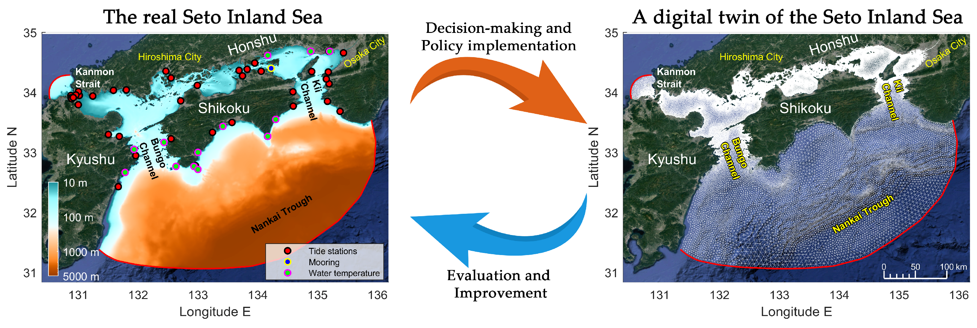
The main purpose of this research is to establish a robust, precise, and high-resolution model of the SIS that can be used as a basis to obtain a digital twin of the SIS. In this early stage, we set the ocean circulation model using SCHISM and validated circulations in the SIS. However, to achieve the purpose of digital twin development, additional modules, such as a wind wave model, sediment transport model, and particle tracking model, should be considered in further work. In addition, when new policies or developments related to oceans are formulated, one of the main concerns is their potential impacts on primary production and marine ecosystems. Negative effects can be especially critical in the SIS because aquaculture is one of the main economic activities in this region. Therefore, one of our goals is to provide various biological indices to monitor these effects. To produce these variables more dependably and accurately in real time, data assimilation is essential to allow possible errors in the model outputs to be corrected using real-world observations. At present, data assimilation is not applied, so it must be implemented in the future. The concept of a digital twin of the SIS and its relationship with the real SIS are illustrated in Figure 11.

Figure 12 depicts the structure of the modeling system designed for developing a digital twin of the SIS. These modules will offer more informative variables, including not only the surface elevation and currents but also waves, sediments, particles such as microplastics and drifting wood, and other objects.

6. Conclusions

A DT is a technology that has grown rapidly with the importance of digital transformation and the emergence of Industry 4.0 from the beginning of the 21st century. Previously, DTs were utilized mainly in manufacturing, aviation, and health care. The use of DTs is expanding dramatically to other large-scale fields, as digital twins of cities, oceans, and the Earth have been constructed.

This study serves as a foundation for establishing a well-organized digital twin system of the SIS. The SCHISM model was applied to a 39-day simulation; these 39 days including the typhoon season, when atmospheric conditions were tough and extreme. To make the model even more robust and accurate, more effort was put into the model parameter settings, such as spatially varying filtering parameters calculated from instability factors and spatially varying grid resolution considering bathymetric gradients. Especially after adopting the filtering parameters, the model was able to transition from the Nankai Trough (4900 m depth) to rivers (3 m depth) without requiring grid nesting, despite grid resolution being changed from 9.8 km to 30 m. These efforts allowed us to seamlessly simulate the river–coastal ocean circulations in and around the SIS. The model presented reasonable validation results in terms of elevations, tidal currents, and temperature, and reproduced the storm surge of approximately 2.37 m in Osaka Bay. There was no previous study where a high-resolution model describing all narrow straits in the SIS was established and validated without grid nesting. The model results within one mesh will be utilized as a main data source consisting of a digital twin of the SIS in the future.

Although the interaction between reality and the model is an essential requirement for the DT system, methods or concepts for facilitating this interaction and establishing a real-time feedback system are still in the early stages of development even globally, particularly in terms of digital twins of oceans. These interactions have the potential to enhance our understanding and enable more accurate predictions, leading to well-informed decision-making, as digital twins can be used to assess and affect new policies and environmental management practices. However, in this study, we were unable to address this aspect. Our efforts were solely on generating a reliable dataset using the model.

The model results were validated in terms of tides, temperatures, and currents. The tidal component outputs showed NRMSE values less than 0.15 and R² values larger than 0.87 at forty-two tidal stations in the SIS. We confirmed that tides propagated all the way inside the SIS, though this effect was not well-reproduced in previous literature. Moreover, the model could reproduce the seasonal and fortnight scale temperature trends shown in the observations.

The current velocities observed in various layers (5, 10, 20, and 30 m) at mooring stations were used to validate the model results. The NRMSE values ranged from 0.11 to 0.17, and the R² values ranged from 0.74 to 0.79. Statistically, the model calculated currents that were approximately 0.05 m/s larger than the observations. However, the slopes of the regression lines were nearly all one, indicating the high reproducibility of the model for velocity variations. The model exhibited high-velocity distributions around narrow straits in the SIS. At the Naruto Strait, famous for its large whirlpools and strong currents, 5 m/s depth-averaged currents were calculated.

The model successfully simulated the storm surge caused by Typhoon Jebi in 2018, accurately calculating the observed surge as the typhoon approached Osaka City. The timing of the surge’s arrival and its spatial distribution were also accurately reproduced by the model, demonstrating the model’s potential for application to other extreme events in the SIS.

According to the terminology discussed in the introduction, our model is currently categorized as a digital model since it simulates pre-existing ocean environments using past data without automatic data exchanges with the real world. However, it is imperative to undertake this fundamental step towards developing a digital twin of an ocean for the eventual realization of fully developed ocean digital twins.

We visualized the validated model results in the three-dimensional domain to demonstrate the concept of a digital twin of the SIS system. This visualization illuminated the bathymetric, circulation, and water temperature characteristics of the SIS and is expected to help various stakeholders, such as marine navigators, decision-makers, and citizens, understand the sea status both easily and intuitively.

Finally, the structure of the modeling system was illustrated to guide the direction of our future study. The digital twin of the SIS discussed in this study is in the very early stage, and more modules will be added to represent wind waves, sediment transport and sedimentation, and particle tracking with the assimilation of oceanic data to produce and provide diverse information to various stakeholders. Then, a platform for the dissemination of this information will also be further developed.