DPGWO Based Feature Selection Machine Learning Model for Prediction of Crack Dimensions in Steam Generator Tubes

Abstract

The selection of an appropriate number of features and their combinations will play a major role in improving the learning accuracy, computation cost, and understanding of machine learning models. In this present work, 22 gray-level co-occurrence matrix features extracted from magnetic flux leakage images captured in steam generator tubes’ cracks are considered for developing a machine learning model to predict and analyze crack dimensions in terms of their length, depth, and width. The performance of the models is examined by considering R² and RMSE values calculated using both training and testing data sets. The F Score and Mutual Information Score methods have been applied to prioritize the features. To analyze the effect of different machine learning models, their number of features, and their selection methods, a Taguchi experimental design has been implemented and an analysis of variance test has been conducted. The dynamic population gray wolf algorithm (DPGWO) has been adopted to select the best features and their combinations. Due to the two contradictory natures of performance metrics, Pareto optimal solutions are considered, and the best one is obtained using Deng’s method. The effectiveness of DPGWO is proved by comparing its performance with Grey Wolf Optimization and Moth Flame Optimization algorithms using the Friedman test and performance indicators, namely inverted generational distance and spacing.

1. Introduction

In nuclear power plants, critical components such as steam generator tubes (SGT), feed water heaters, and pressure vessels have stringent design requirements due to the high temperature, pressure, and radiation-exposing environment, which induce stress corrosion cracking, pitting, fouling, and mechanical fretting [1]. Apart from that, steam generator tube rupture (SGTR) leads to the inevitable release of radiation into the environment [2]. For the safety and reliable operation of the plant, it is necessary to go for online monitoring and periodic inspection [3,4]. Non-destructive testing (NDT) is a mode of testing that has been adopted by industries for more than a decade to test mass-manufactured products for anomalies. This process is increasingly being used by sectors such as aerospace, oil and gas, petroleum, nuclear, and construction industries [5,6,7]. More part failures occur due to the complexity of the devices produced. To avoid such things, NDT findings forecast failure and enhance the safety and economy of enterprises. Sumptuous non-destructive evaluation techniques have been established for major systems such as power plants and airplanes to confirm the durability of the NDT test and their safety. Singh et al. [8] proposed the magnetic flux leakage (MFL) technique to identify the localized faults in the SGT. Zhang et al. [9] implemented the MFL technique to detect both shallow surface and deep sub-surface defects in ferromagnetic materials. Suresh et al. [10,11] suggested the MFL approach for the detection of defects and subsurface cracks in small-diameter SGT. The experimental setup for the measurement of MFL is detailed in Suresh et al. [10]. Daniel et al. [12] designed an ANN model to forecast the SGT’s defect in terms of the length, breadth, and depth of the crack by providing the gray-level co-occurrence matrix (GLCM) information extracted from the MFL images.

Wang et al. [13] studied a detailed review of the application of ML models in predicting the outcomes of stroke with structured data. The random forest (RF) ML algorithm has been implemented to predict the outcome of endovascular treatment [14] and acute stroke [15] and improve prediction accuracy in Ischemic stroke patients. Decision tree (DT) and extreme gradient boosting (XGB) ML algorithms were implemented to improve the accuracy of the prediction of Ischemic stroke patients [16].

In ML, feature selection, a method of selecting independent parameters, reduces the computation time and complexity of the problem by eliminating irrelevant, not-useful, and redundant features. Due to its combinatorial nature, feature selection is treated as a non-polynomial hard problem, which creates the opportunity for the researchers to implement meta-heuristic algorithms. Devi et al. [17] proposed a new variant of the Golden Jackel Optimization (GJO) algorithm called Improved GJO (IGJO) to solve the feature selection problem in ML. Qaraad et al. [18] introduced quadratic interpolation with a salp swarm-based local escape operator in the feature selection of 19 datasets and conducted Friedman and Wilcoxon tests to analyze the results. Houssein et al. [19] implemented a centroid mutation-based search and rescue optimization algorithm for feature selection in 15 disease data sets with different feature sizes extracted from the UCI machine learning repository and compared the performance with six existing meta-heuristic algorithms. Filter-based and wrapper-based techniques are the two basic categories under which feature selection may be classified [20,21]. While the wrapper-based strategy bases its evaluation of the solution throughout the searching and optimization procedures on the learning algorithm, the filter-based approach uses the correlation between the data and the relevant class label without consulting the learning algorithm. The wrapper-based technique is the most frequently employed feature selection method as compared to the less computationally expensive filter-based approach due to its higher performance accuracy [22,23].

In this work, the ML model is to be developed to predict the SGT’s defect in terms of length, width, and depth of crack from the given gray level co-occurrence matrix feature from the MFL image. The feature selection method and the number of selected features will affect the performance of the ML models. The R² and root mean square error (RMSE) values are considered metrics to measure the performance of the ML models. Multiple contradictory performance measures require the conversion of multiple objectives into a single objective, which initiated the implementation of a multi-criterion decision-making method, namely Deng’s method. The dynamic population gray wolf optimization (DPGWO) algorithm is implemented to select the number of features and their combinations to minimize the prediction error. The effectiveness of the DPGWO algorithm is proved by comparing its performance with the gray wolf optimization (GWO) Algorithm [24] and moth flame optimization algorithm (MFO) [25] by implementing a non-parametric Friedman test [25] and performance indicators.

The paper is organized as follows. Section 2 describes the problem statement, and Section 3 describes the proposed methodology and the various stages, namely prioritizing the features, Taguchi orthogonal array experimental design [25], analysis of Variance (ANOVA) Test, and meta-heuristic algorithms for feature selection involved in solving the problem. Section 4 deals with the results and discussion, including a comparison of the performance of the DPGWO algorithm with the MFO and GWO algorithms. Finally, the conclusion part of the paper gives future scope.

2. Problem Statement

Any model must be appropriately selected to match the requirements of the application. Decision-makers analyze the behavior of data using prediction models. Regression models, artificial neural networks, and support vector machines are a few techniques used to build prediction models. Each technique has its own pros and cons based on the size of the dataset. Recently, machine learning techniques have assisted researchers in developing more accurate prediction models. The type of machine learning (ML) model will differ from problem to problem. The same ML model may not give similar performance across applications. Hence, the selection of a suitable ML model for the given problem is a challenging task.

Apart from that, the selection of appropriate features will play a major role in improving the learning accuracy, computation cost, and understanding of the model. Overfitting of models is one of the major problems that will reduce the application of ML in various fields. The problem considered in this work will be developing an accurate ML model with a smaller number of features to predict the crack dimensions from 22 GLCM features extracted from 105 MFL crack images presented by Daniel et al. [12].

3. Methodology

The main focus of the present work is to implement a suitable ML Model with an appropriate selection of features and their combinations to predict the crack dimensions more accurately as compared with the existing ANN model. Daniel et al. [12] from the given 22 GLCM features extracted from 115 MFL crack images. This has been carried out in four stages. In the first stage, the features are prioritized based on F Score (FS) and Mutual Information Score (MIS) values. L16 Taguchi orthogonal array design [25] has been constructed by considering feature selection methods (FSM), machine learning models (MLM), and number of features as parameters and R² and RMSE values as response values. For each experiment, python codes are executed using the corresponding MLM, FSM, and target number of features as determined by the Taguchi array to determine the corresponding R² and RMSE values for both training and test data sets. To analyze the effect of parameters and their interaction on the response values, an ANOVA test has been carried out in the third stage. The responses, namely R² and RMSE values, for the training and testing data sets, are different for each experiment, which is similar to different alternatives among multiple design problems. To select the best design, these multiple responses are to be converted into a single value. Hence, in this work, a similarity-based multi-criterion ranking method called Deng’s method [26] is introduced to select the best ML model in the third stage. In the fourth stage, meta-heuristic algorithms, namely MFO, GWO, and DPGWO, a new variant of GWO proposed in this work, have been implemented to select the number of features and their combinations. Also, Performance indicators and Friedman’s test have been conducted in the fourth stage to prove the effectiveness of the DPGWO, along with statistical analysis to confirm the results. The proposed methodology is shown in Figure 1. The step-by-step algorithm of the proposed work is given below.

Step 1:

Read the GLCM features and their corresponding crack dimension datasets.

Step 2:

Prioritize the features’ order based on

(a)

Mutual Information Score (MIS)

(b)

F Score (FS)

Step 3:

Arrange the features based on MIS.

Step 4:

Select the first 15 features and fix one of the crack’s dimensions as the target value.

Step 5:

Set a machine learning model and select R² and RMSE as performance metrics of the machine learning model.

Step 6:

Set the size of a training data set, and based on that, separate the training and testing data sets along their target values.

Step 7:

Fit the ML model for the data set and predict both training and testing target values.

Step 8:

Compute the response values (performance metrics, namely R² and RMSE) of the ML model for both the training and testing data sets.

Step 9:

Repeat steps 5 to 8 by changing the different ML models.

Step 10:

Repeat steps 4 to 9 by changing the number of features to 17, 19, and 21.

Step 11:

Repeat steps 3 to 10 by arranging the features based on the F Score.

Step 12:

Conduct an ANOVA and statistical test to test the significance of the parameters on the response values.

Step 10:

Implement Deng’s method to select the best machine learning model based on R2 and RMSE values.

Step 11:

Tune the hyper-parameters of the best machine learning model.

Step 12:

Implement the MFO, GWO, and DPGWO algorithms by randomly selecting the given features along with their target values between 15 and 21.

Step 13:

Compare the performance of algorithms using performance indicators (Inverted Generational Distance and Spacing) and Friedman’s Test. Select the best number of features and their combinations.

Step 14:

Repeat the steps from 3 to 15 for other dimensions of the crack, like crack depth and crack width.

3.1. Stage 1: Prioritizing the Features

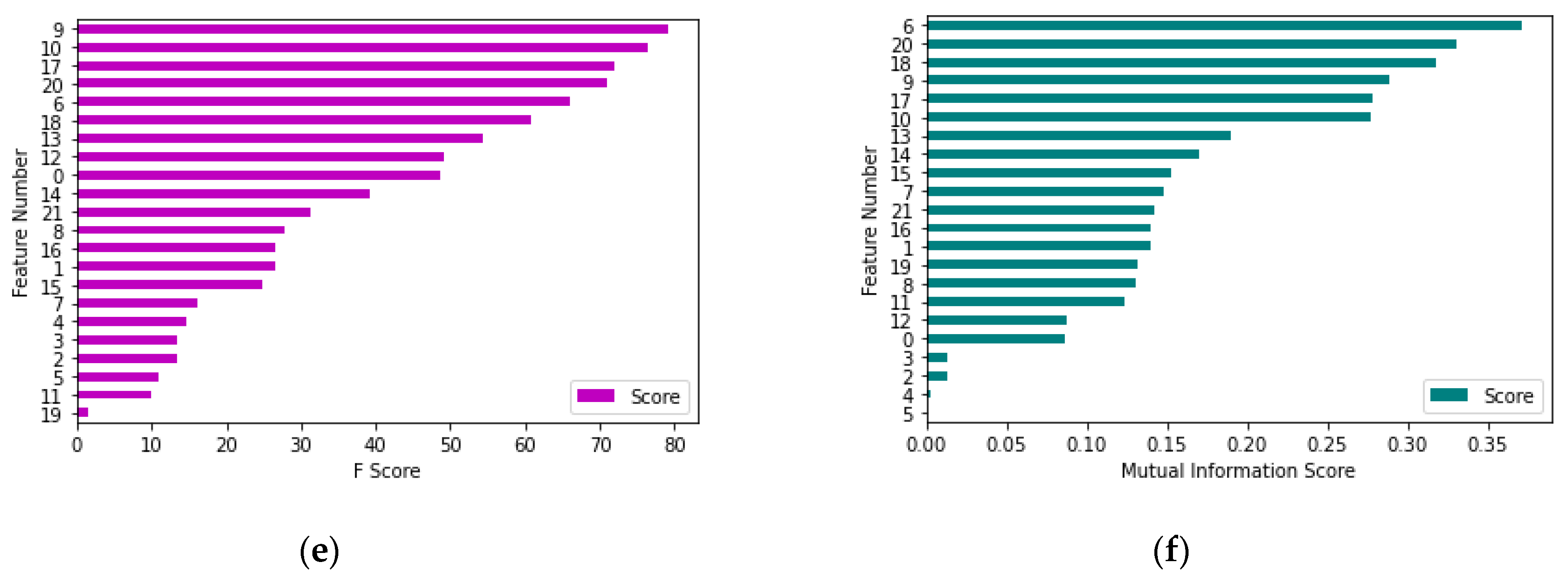
Consideration of all features in machine learning may lead to poor performance, excess computation time, and overfitting of the prediction model. To avoid this, feature selection techniques have been used in ML. Since the wrapper method of feature selection is an iterative process and slow in nature, in this work two filter methods, namely, the F score (FS) and the mutual information score (MIS), have been introduced for selection. In the F score method, features are selected statistically by identifying the relationship between parametric features and target features, whereas in the mutual information score method, features are selected based on their entropy.

Table 1. GLSM Feature Details (Daniel et al. [12]).

FNo.	FName	Feature Name
0	UNF	Energy/Uniformity
1	ETR	Entropy
2	DSL	Dissimilarity
3	CST	Contrast
4	ID	Inverse Difference
5	CN	Correlation
6	H	Homogeneity
7	AC	Auto correlation
8	CS	Cluster shade
9	CP	Cluster prominence
10	MP	Maximum Probability
11	SS	Sum of squares
12	SA	Sum average
13	SV	Sum Variance
14	SE	Sum entropy
15	DV	Difference Variance
16	DE	Difference entropy
17	IMC (1)	Information measure of correlation1
18	IMC (2)	Information measure of correlation 2
19	MCC	Maximal Correlation Coefficient
20	INN	Inverse Difference Normalized
21	IDN	Inverse different moment normalized

FNo.—Feature Number and Fname—Feature Name.

represents the list of 22 GLCM features extracted from MFL images of crack dimensions. Figure 2 represents the prioritized features of crack dimensions. It is understood that in Figure 2a, the 3rd feature is given priority and the 2nd feature is given least the priority in the F-Score-based prioritized method, whereas in the MIS method, the 1st feature has first priority and the 19th feature has the least priority in crack length prediction. In crack width prediction, the 7th feature has first priority in both prioritized methods. Different features, namely the 20th and 6th features, have the least priority in crack depth prediction [27].

3.2. Stage 2: Taguchi Orthogonal Array Experimental Design for ML Model Selection

In this work, a total of six different ML models have been used, in which a different combination of four models is considered for each crack dimension. The ML models’ names are described in

Table 2. List of Machine Learning (ML) Models Used in Crack Length.

Model	Name
DT	Decision Tree Regressor
LoR	Logistic Regressor
LiR	Linear Regressor
XGB	Extreme Gradient Booster
ABR	Adaptive Booster Regressor
RF	Random Forest Regressor

. The parameters and their levels considered for crack length are represented in

Table 3. Parameters and Its Level for Crack Length.

Parameter	No. of Levels	Levels
		1	2	3	4
FSM	2	FS	MIS
MLM	4	DT	LiR	LoR	XGB
NoF	4	15	17	19	21

. The ML models considered for crack depth and crack width are represented in

Table A1. Parameters and Its Level—Crack Depth.

Parameter	No. of Levels	Levels
		1	2	3	4
FSM	2	FS	MIS
MLM	4	ABR	LiR	RF	XGB
NoF	4	15	17	19	21

and

Table A4. Parameters and Its Level—Crack Width.

Parameter	No. of Levels	Levels
		1	2	3	4
FSM	2	FS	MIS
MLM	4	ABR	LiR	RF	XGB
NoF	4	15	17	19	21

.

Table 4. L16 OA—Performance of ML for Crack Length.

E.No.	FSM	MLM	NoF	R2Tr	R2Tt	RMSETr	RMSETt	Deng’s Value
1	FS	DT	15	0.2619	0.3737	0.9684	1.4000	0.4569
2	FS	DT	17	0.1998	0.4572	1.0000	1.3000	0.4771
3	MIS	DT	19	0.6100	0.1434	1.0278	1.6440	0.4879
4	MIS	DT	21	0.5940	0.1429	1.0282	1.6446	0.5040
5	FS	LiR	15	0.9596	0.6091	0.2346	1.2090	0.4434
6	FS	LiR	17	0.9592	0.6209	0.2389	1.1815	0.4616
7	MIS	LiR	19	0.9221	0.6109	0.3917	1.1977	0.4643
8	MIS	LiR	21	0.9078	0.5437	0.4225	1.2860	0.4248
9	MIS	LoR	15	0.6002	0.1449	0.8200	1.6425	0.5484
10	MIS	LoR	17	0.6120	0.1441	0.8150	1.6433	0.5360
11	FS	LoR	19	0.5860	0.1434	0.8008	1.6441	0.5324
12	FS	LoR	21	0.3960	0.1430	0.8400	1.6445	0.5408
13	MIS	XGB	15	0.8652	0.8646	0.4410	0.6942	0.6073
14	MIS	XGB	17	0.8757	0.8705	0.4055	0.6869	0.6444
15	FS	XGB	19	1.0000	0.5988	0.0005	1.1801	0.6263
16	FS	XGB	21	1.0000	0.5841	0.0006	1.2013	0.6326

represents the experimental parameter settings of the L16 Taguchi orthogonal array for the given combination of levels of parameters mentioned in Table 3, obtained using Minitab 19 Software, where 16 represents the minimum number of experimental runs required to conduct the experiments and to find the best parameter settings [28]. For each experimental run corresponding to its parameter settings, Python code has been executed for the training data set with a sample size of 95 images’ features and tested with a data size of 20 images. The performance of the ML model is recorded for each experiment based on the R² and RMSE values of both the training and testing data sets. Deng’s method has been implemented to select the best ML model based on the overall performance index calculated using R² and RMSE values, which are listed in Table 4. L16 Taguchi orthogonal array and Deng’s values for crack depth and crack width are presented in

Table A2. L16 OA—Performance of ML for Crack Depth.

E.No.	FSM	MLM	NoF	R2Tr	R2Tt	RmseTr	RmseTt	Deng’s Value
1	FS	ABR	15	0.7741	0.0441	1.3924	3.0091	0.3319
2	FS	ABR	17	0.8537	0.1680	1.2802	3.3972	0.4154
3	MIS	ABR	19	0.8699	0.0221	1.1833	3.1780	0.3480
4	MIS	ABR	21	0.9154	0.0446	0.9110	3.2148	0.3941
5	FS	LiR	15	0.5956	0.3609	1.8665	3.5540	0.4292
6	FS	LiR	17	0.6049	0.2698	1.8390	3.3689	0.3965
7	MIS	LiR	19	0.6883	0.4080	1.6204	3.6648	0.4693
8	MIS	LiR	21	0.7274	0.2882	1.5332	3.5175	0.4361
9	MIS	RF	15	0.9207	0.0444	0.8105	3.1208	0.4061
10	MIS	RF	17	0.9228	0.0584	0.7603	3.0285	0.4208
11	FS	RF	19	0.9330	0.0469	0.6982	3.2378	0.4224
12	FS	RF	21	0.9412	0.0455	0.6224	3.0668	0.4325
13	MIS	XGB	15	1.0000	0.4452	0.0006	3.6458	0.6737
14	MIS	XGB	17	1.0000	0.4829	0.0005	3.7246	0.6806
15	FS	XGB	19	1.0000	0.5153	0.0006	3.9049	0.6836
16	FS	XGB	21	1.0000	0.4663	0.0004	3.7602	0.6761

and

Table A5. L16 OA—Performance of ML for Crack Width.

E.No.	FSM	MLM	NoF	R2Tr	R2Tt	RMSETr	RmseTt	Deng’s Value
1	FS	ABR	15	0.8447	0.2031	0.1349	0.3008	0.4569
2	FS	ABR	17	0.8633	0.2435	0.1240	0.2896	0.4771
3	MIS	ABR	19	0.8573	0.3026	0.1271	0.2798	0.4879
4	MIS	ABR	21	0.8789	0.3411	0.1191	0.2724	0.5040
5	FS	LiR	15	0.6983	0.3227	0.1795	0.2604	0.4434
6	FS	LiR	17	0.7047	0.3961	0.1781	0.2391	0.4616
7	MIS	LiR	19	0.7382	0.3611	0.1663	0.2561	0.4643
8	MIS	LiR	21	0.7632	0.1582	0.1518	0.2909	0.4248
9	MIS	RF	17	0.9351	0.3889	0.0820	0.2648	0.5484
10	MIS	RF	19	0.9361	0.3163	0.0800	0.2822	0.5360
11	FS	RF	19	0.9328	0.2949	0.0800	0.2665	0.5324
12	FS	RF	21	0.9337	0.3332	0.0793	0.2635	0.5408
13	MIS	XGB	15	1.0000	0.1967	0.0006	0.2825	0.6073
14	MIS	XGB	17	1.0000	0.4196	0.0006	0.2440	0.6444
15	FS	XGB	19	1.0000	0.3050	0.0005	0.2688	0.6263
16	FS	XGB	21	1.0000	0.3386	0.0006	0.2570	0.6326

.

3.3. Stage 3: ANOVA Test

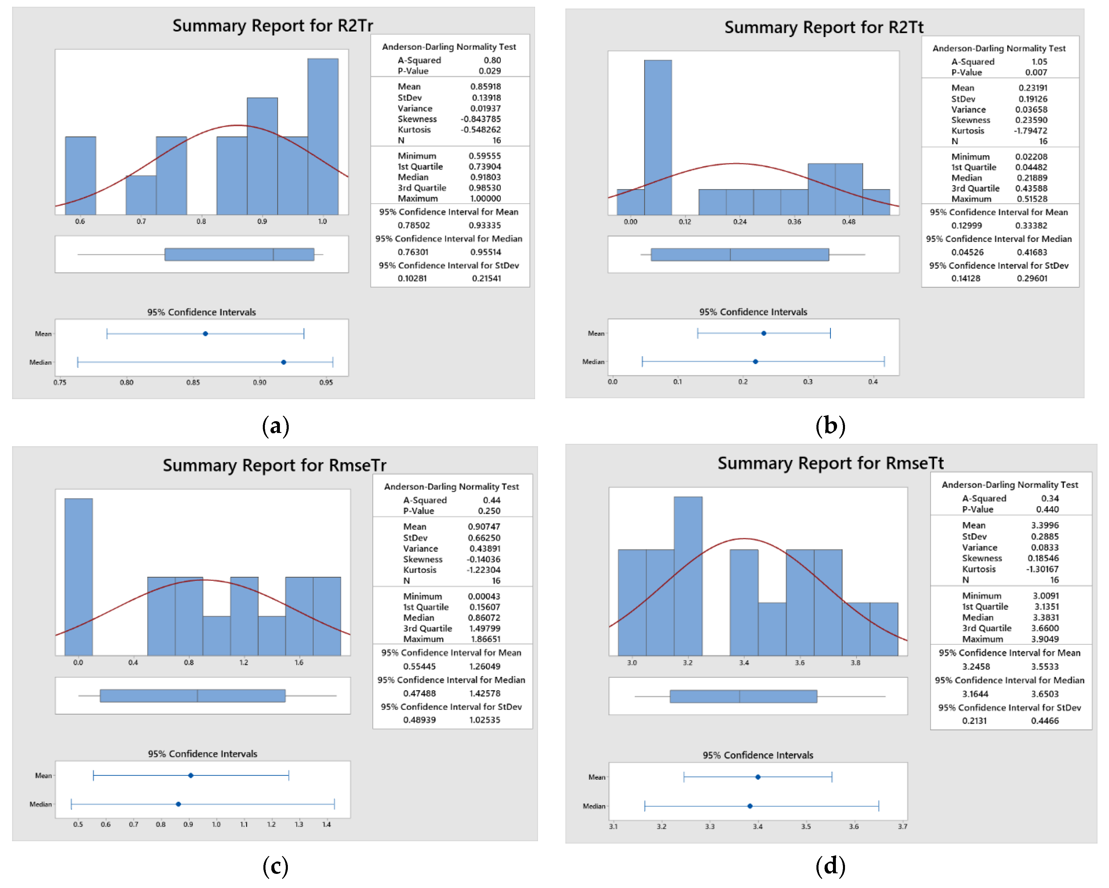
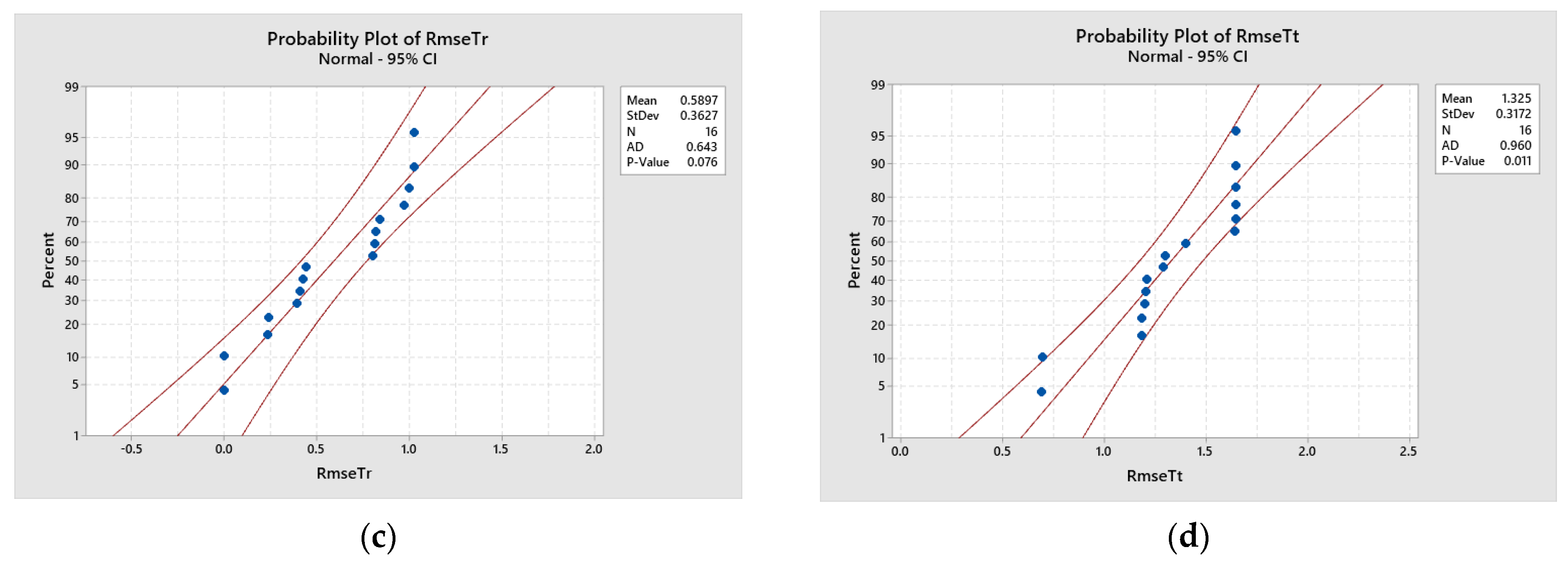
The ANOVA Test is used to analyze the differences among the means of different groups using variance and to prove which groups are statistically significant. To prove that the performance is significantly different for various ML models, an ANOVA test [24] is implemented in this work. Figure 3 represents the probability plot of performance measures of the ML model obtained by executing the Python codes. It is understood that the values of R² and RMSE of both training and testing are within the 95% confidence interval and that their probability values are greater than 0.005. This shows that the experimentation results are acceptable for crack length prediction. Similarly, for crack depth and crack width, the p-value shown in Figure A1 and

Table A6. Statistical Analysis of ML Models’ Performance for Crack Width Prediction.

Variable	Mean	StDev	Variance	Minimum	Q1	Median	Q3	Maximum	Range	p-Value
R2Tr	0.8804	0.1061	0.0113	0.6983	0.7836	0.9058	0.9840	1.0000	0.3017	0.0950
R2Tt	0.3076	0.0743	0.0055	0.1582	0.2564	0.3195	0.3561	0.4196	0.2614	0.3030
RmseTr	0.0940	0.0648	0.0042	0.0005	0.0203	0.1006	0.1476	0.1795	0.1790	0.0750
RmseTt	0.2699	0.0170	0.0003	0.2391	0.2579	0.2676	0.2825	0.3008	0.0617	0.9400

is greater than 0.005, which reveals that the experimental results obtained are acceptable.

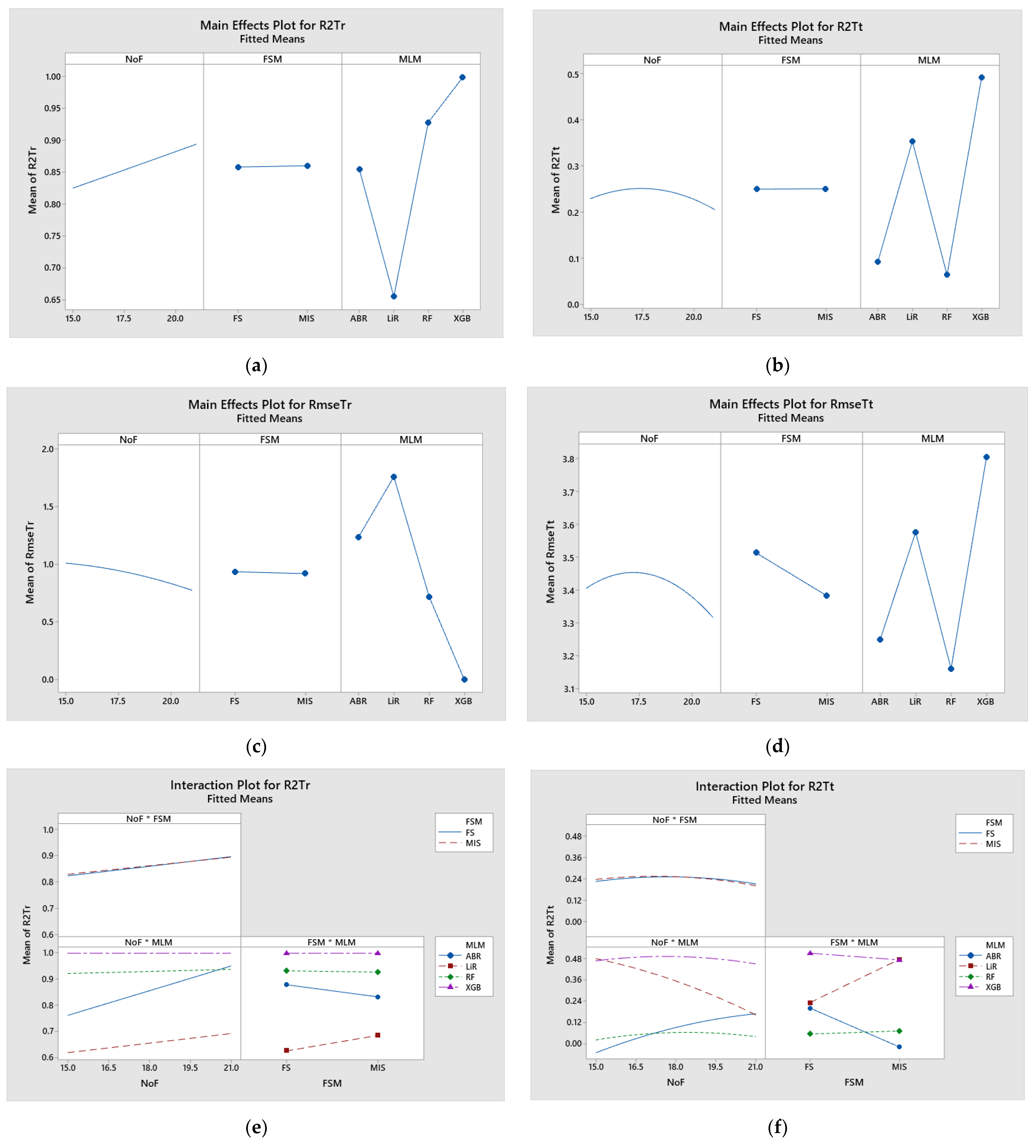
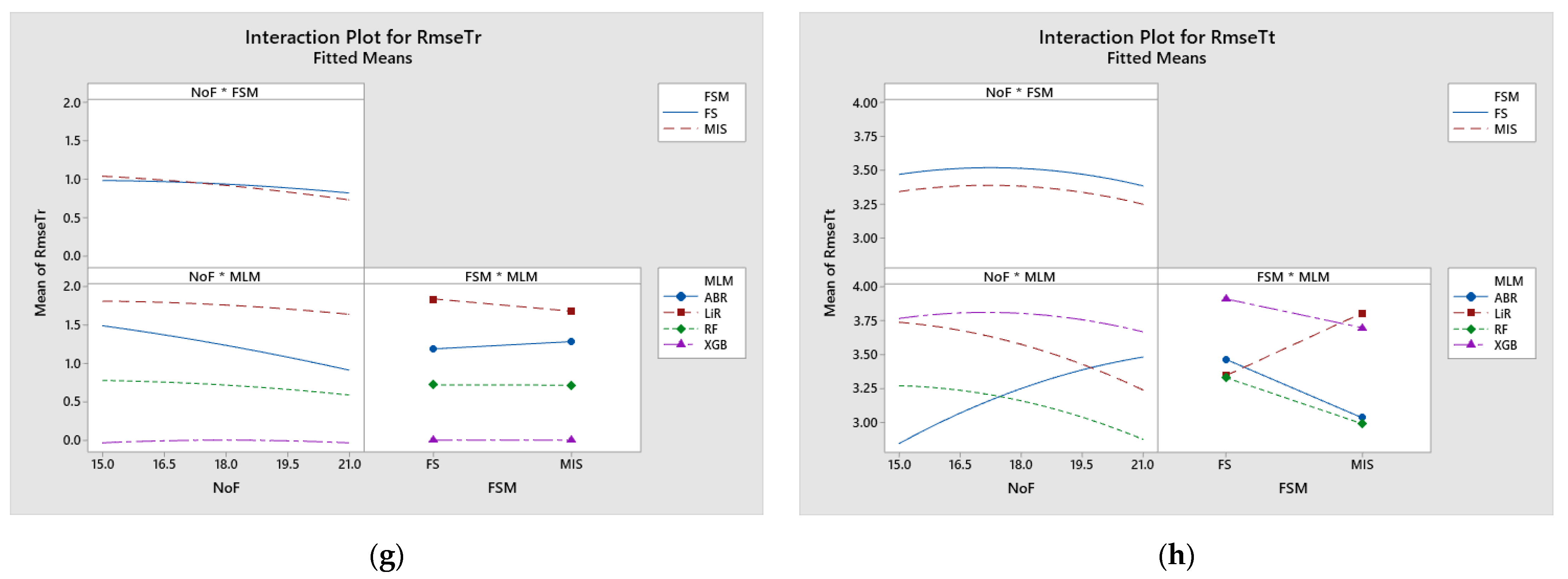
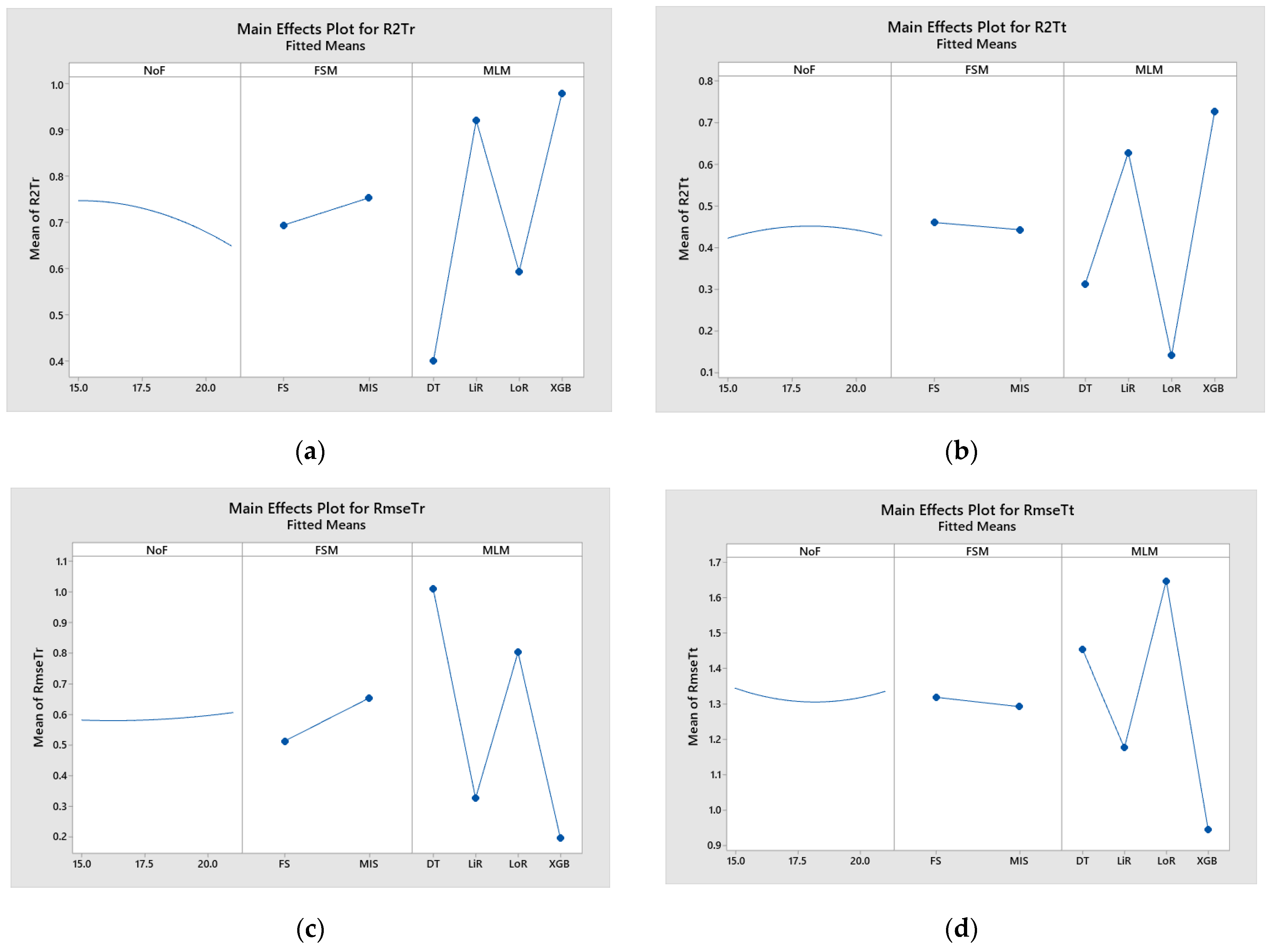
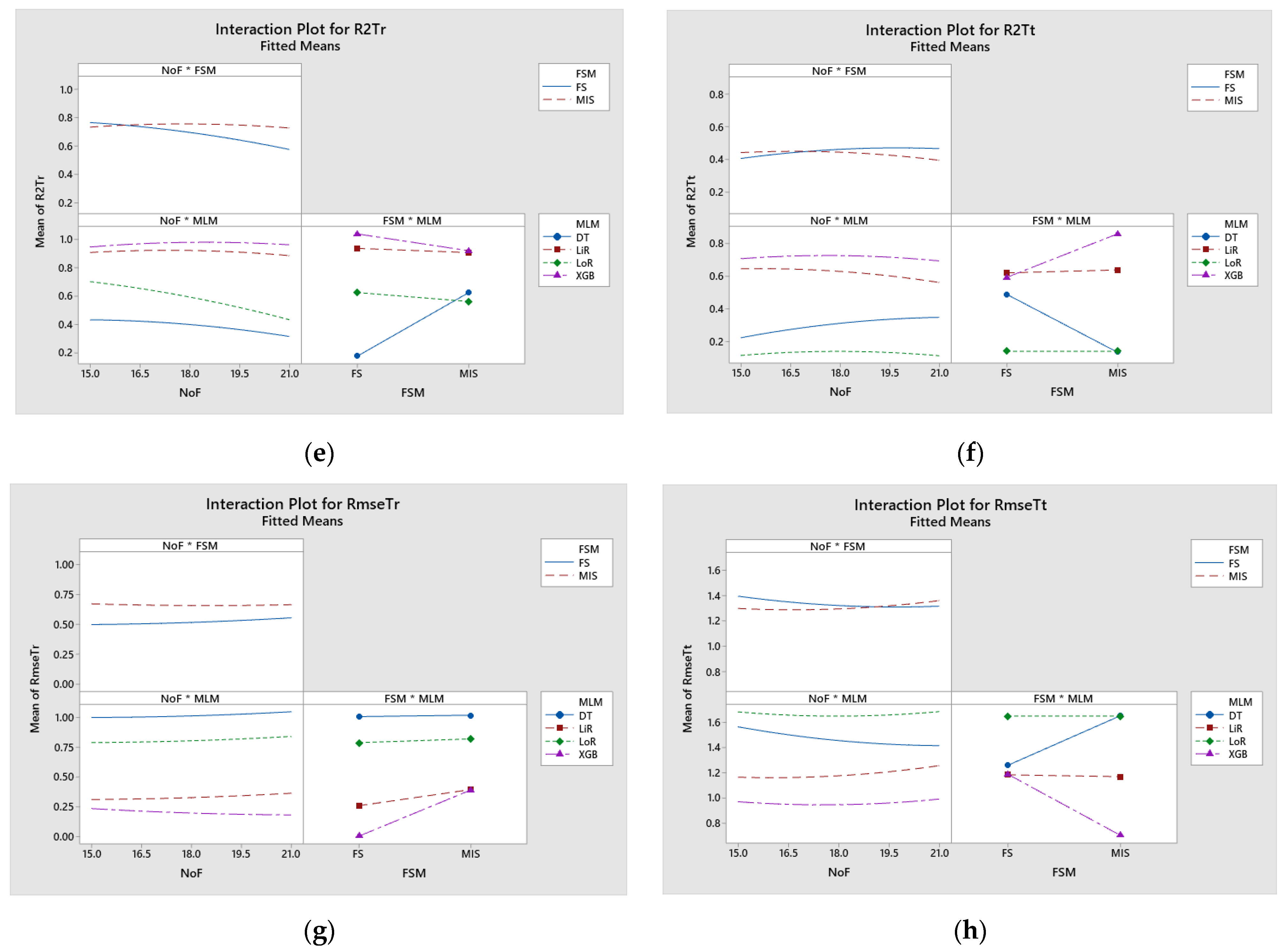
The main and interaction effect plots of parameters are depicted in Figure 4a–h for crack length prediction. It is inferred from Figure 4a,b that the mean value of R2Tr is higher when the parameters are MIS, 15, and XGB, whereas in R2Tt the parameters are FS and 18, respectively. It is understood from Figure 4c,d, that for getting the lower mean value of RMSETr and RMSETt, the parameters are to be set in a different way than R2Tr and R2Tt. From Figure 4e,f, it is noted that increasing the NoF value decreases the R2Tr value for all ML models, whereas in R2Tt except MLM and DT in all other models, it increases. Using XGB, a lower RMSE is reported in Figure 4g,h.

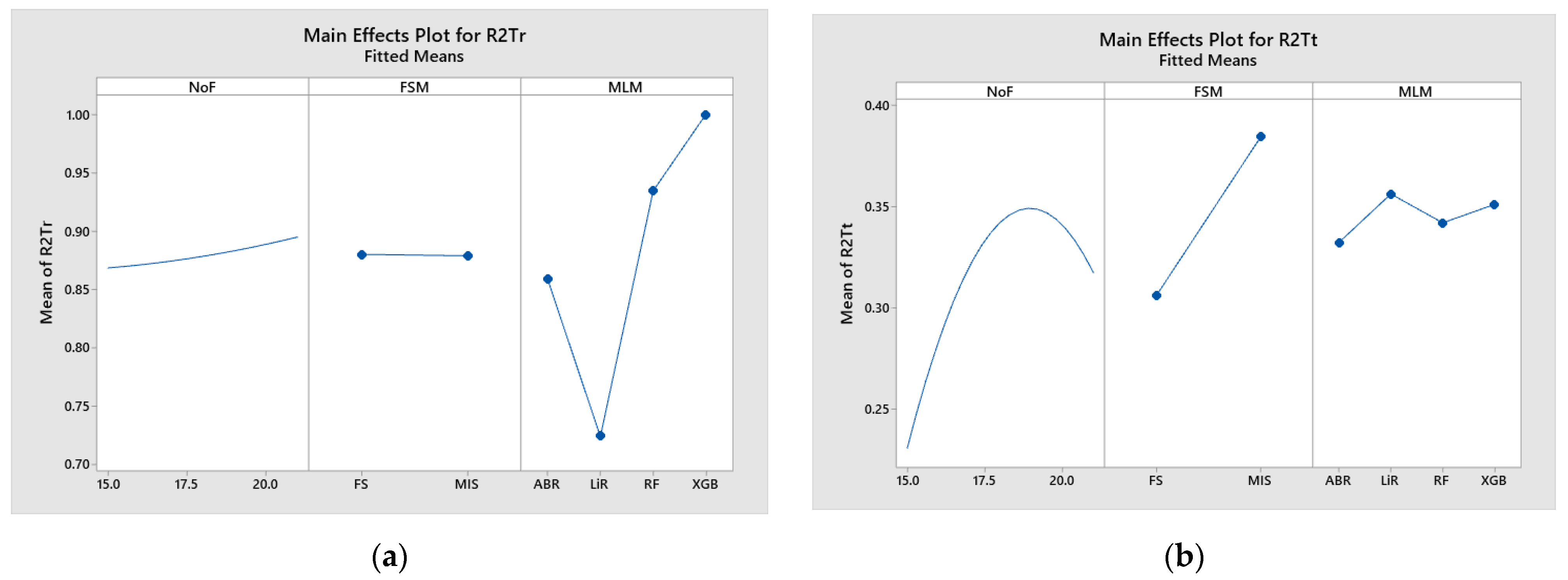
The main and interaction effects plots for crack depth and width are shown in Figure A2a–h and Figure A3a–h. It is observed that different parameter settings are required for getting an individual’s optimum response value. Hence, in this work, Deng’s method is introduced to select the best parameter settings based on R2Tr, R2Tt, RMSETr, and RMSETt values. It is inferred that FS, 19, and XGB are the optimum parameters for the highest Deng’s value, which will give optimum response values.

The p-values of factors and their interactions for the training dataset, except for the interaction between FSM and MLM, are all greater than 0.05 in

Table 5. ANOVA for Crack Length Prediction.

Source	DF	R2Tr				R2Tt
		Adj SS	Adj MS	F-Value	p-Value	Adj SS	Adj MS	F-Value	p-Value
Regression	13	1.0433	0.0803	31.9400	0.0310	1.0445	0.0803	2780.6000	0.0000
NoF	1	0.0008	0.0008	0.3300	0.6250	0.0033	0.0033	113.4200	0.0090
FSM	1	0.0001	0.0001	0.0500	0.8480	0.0000	0.0000	0.4700	0.5640
MLM	3	0.0051	0.0017	0.6700	0.6450	0.0057	0.0019	65.8000	0.0150
NoF*NoF	1	0.0020	0.0020	0.8100	0.4640	0.0021	0.0021	72.5800	0.0130
NoF*FSM	1	0.0037	0.0037	1.4900	0.3470	0.0013	0.0013	44.0600	0.0220
NoF*MLM	3	0.0053	0.0018	0.7000	0.6320	0.0025	0.0008	28.7400	0.0340
FSM*MLM	3	0.0414	0.0138	5.4900	0.1580	0.0394	0.0131	454.0900	0.0020
Error	2	0.0050	0.0025			0.0001	0.0000
Total	15	1.0484				1.0446
		RMSETr				RMSETt
		Adj SS	Adj MS	F-Value	p-Value	Adj SS	Adj MS	F-Value	p-Value
Regression	13	1.9731	0.1518	711.9000	0.0010	1.5092	0.1161	1722.1200	0.0010
NoF	1	0.0002	0.0002	0.7300	0.4820	0.0057	0.0056	83.7600	0.0120
FSM	1	0.0005	0.0005	2.2300	0.2740	0.0000	0.0000	0.1500	0.7340
MLM	3	0.0057	0.0019	8.8700	0.1030	0.0063	0.0021	31.2100	0.0310
NoF*NoF	1	0.0004	0.0004	1.6500	0.3270	0.0037	0.0037	55.4600	0.0180
NoF*FSM	1	0.0005	0.0004	2.0900	0.2850	0.0022	0.0022	32.8400	0.0290
NoF*MLM	3	0.0009	0.0003	1.4000	0.4410	0.0034	0.0011	16.8800	0.0560
FSM*MLM	3	0.0179	0.0060	27.9500	0.0350	0.0778	0.0259	384.5400	0.0030
Error	2	0.0004	0.0002			0.0001	0.0001
Total	15	1.9735				1.5093

, which confirms that none of the factors and their interactions influence the performance of ML Models. In the testing dataset, it is identified that NoF and MLM are the influencing parameters. A similar representation is observed in crack depth prediction, which is shown in

Table A3. ANOVA for Crack Depth Prediction.

Source	DF	R2Tr				R2Tt				RMSETr				RMSETt
		Adj SS	Adj MS	F-Value	p-Value	Adj SS	Adj MS	F-Value	p-Value	Adj SS	Adj MS	F-Value	p-Value	Adj SS	Adj MS	F-Value	p-Value
Regression	13	0.29005	0.02231	87.17000	0.01100	0.54741	0.04211	65.07000	0.01500	6.58227	0.50633	753.53000	0.00100	1.22728	0.09441	8.76000	0.10700
NoF	1	0.00018	0.00018	0.70000	0.49100	0.00530	0.00530	8.20000	0.10300	0.00054	0.00054	0.81000	0.46300	0.03826	0.03826	3.55000	0.20000
FSM	1	0.00001	0.00001	0.02000	0.89300	0.00028	0.00028	0.44000	0.57700	0.00329	0.00329	4.90000	0.15700	0.00192	0.00192	0.18000	0.71400
MLM	3	0.00416	0.00139	5.42000	0.16000	0.02247	0.00749	11.57000	0.08100	0.05840	0.01947	28.97000	0.03400	0.10052	0.03351	3.11000	0.25300
NoF*NoF	1	0.00000	0.00000	0.00000	0.98300	0.00336	0.00336	5.20000	0.15000	0.00377	0.00377	5.60000	0.14200	0.02372	0.02372	2.20000	0.27600
NoF*FSM	1	0.00001	0.00001	0.03000	0.88400	0.00005	0.00005	0.08000	0.80900	0.00236	0.00236	3.51000	0.20200	0.00001	0.00001	0.00000	0.98100
NoF*MLM	3	0.00241	0.00080	3.14000	0.25100	0.01630	0.00543	8.39000	0.10800	0.01977	0.00659	9.81000	0.09400	0.08768	0.02923	2.71000	0.28100
FSM*MLM	3	0.00113	0.00038	1.47000	0.42900	0.02182	0.00727	11.24000	0.08300	0.00680	0.00227	3.37000	0.23700	0.09859	0.03287	3.05000	0.25700
Error	2	0.00051	0.00026			0.00129	0.00065			0.00134	0.00067			0.02154	0.01077
Total	15	0.29057				0.54870				6.58361				1.24882

. In

Table A7. ANOVA for Crack Width Prediction.

Source	DF	R2Tr				R2Tt				RMSETr				RMSETt
		Adj SS	Adj MS	F-Value	p-Value	Adj SS	Adj MS	F-Value	p-Value	Adj SS	Adj MS	F-Value	p-Value	Adj SS	Adj MS	F-Value	p-Value
Regression	13	0.16896	0.01300	835.7	0.001	0.06584	0.00507	0.6	0.773	0.06290	0.00484	298.85	0.003	0.00383	0.00030	1.15	0.556
NoF	1	0.00000	0.00000	0.19	0.703	0.01402	0.01402	1.66	0.326	0.00000	0.00000	0.02	0.896	0.00049	0.00049	1.93	0.299
FSM	1	0.00005	0.00005	3.43	0.205	0.00126	0.00126	0.15	0.736	0.00002	0.00002	0.91	0.442	0.00011	0.00011	0.42	0.584
MLM	3	0.00149	0.00050	31.84	0.031	0.02175	0.00725	0.86	0.577	0.00045	0.00015	9.18	0.1	0.00073	0.00024	0.95	0.55
NoF*NoF	1	0.00003	0.00003	1.79	0.313	0.01175	0.01175	1.39	0.359	0.00001	0.00001	0.3	0.637	0.00038	0.00038	1.5	0.346
NoF*FSM	1	0.00002	0.00002	1.38	0.36	0.00118	0.00118	0.14	0.744	0.00001	0.00001	0.41	0.589	0.00011	0.00011	0.44	0.576
NoF*MLM	3	0.00033	0.00011	7.13	0.126	0.01897	0.00633	0.75	0.615	0.00007	0.00002	1.45	0.434	0.00059	0.00020	0.78	0.606
FSM*MLM	3	0.00020	0.00007	4.28	0.195	0.00723	0.00241	0.29	0.836	0.00003	0.00001	0.62	0.666	0.00056	0.00019	0.73	0.624
Error	2	0.00003	0.00002			0.01686	0.00843			0.00003	0.00002			0.00051	0.00026
Total	15	0.16899				0.08270				0.06294				0.00434

, it is noted that only MLM influences the performance of the prediction of crack width.

Table 6. Best ML Model and Number of Features for Crack Dimension Prediction in Taguchi Method (TM).

Characteristic	FSM	MLM	NoF	R2Tr	R2Tt	RMSETr	RMSETt	Deng’s Value
Length	MIS	XGB	17	0.8757	0.8705	0.4055	0.6869	0.6444
Depth	FS	XGB	19	1.0000	0.5153	0.0006	3.9049	0.6836
Width	MIS	XGB	17	1.0000	0.4196	0.0006	0.2440	0.6444

represents the best ML model, the feature selection method, and the number of features for each crack dimension. It is understood that out of the six ML models, XGB performed well for all the crack dimensions. For comparison purposes, the optimum parameters obtained by the desirability function method using Minitab R19 Software are given in

Table 7. Optimum Parameters for Crack Dimensions using Composite Desirability Method (DM).

Solution for	FSM	ML	NoF	R2Tr—Fit	R2Tt—Fit	RMSETr—Fit	RMSETt—Fit	Composite Desirability
Crack Length	MIS	XGB	17	0.890569	0.875854	0.387879	0.655271	0.868386
Crack Depth	FS	XGB	21	0.999998	0.621851	0.0199202	3.39233	0.840767
Crack Width	MIS	XGB	19	0.999706	0.679007	0.0006879	0.231555	0.887385

.

Table 8. List of Hyper Parameters and their Levels.

Parameters	Levels
	1	2	3	4	5
n_estimators	100	500	900	1100	1500
base_score	0.25	0.5	0.75	1
learning_rate	0.05	0.1	0.15
Booster	gbtree	Gblinear

represents the list of hyper parameters [15] considered for tuning the performance of the XGB ML model. ‘RandomizedSearchCV’ function is used in Python to get the best hyper parameters for crack dimensions, and the same is presented in

Table 9. Optimum Hyper Parameters of XGB for Crack Dimensions.

Parameters	Crack Dimensions
	Length	Depth	Width
n_estimators	500	1500	100
base_score	1	0.75	1
learning_rate	0.05	0.15	0.05
Booster	Gblinear	gblinear	gbtree

.

3.4. Stage 4: Meta-Heuristic Algorithms for Feature Selection

3.4.1. Gray Wolf Optimization

The GWO algorithm mimics the natural and social behavior of gray wolves in hunting [24]. It is a metaheuristic method used for solving several optimization issues, including signal processing, feature selection, and image processing. GWO was initially designed for one objective problem without constraint [24]. The following variants of GWO were found in a detailed literature review carried out by Mirjalili et al. [27].

• Cross-over and mutation operators to solve economic dispatch problems.
• Different penalty functions are used to solve constrained engineering problems.
• Tournament selection and modified augmented Lagrangian multiplier methods to handle constraint problems.
• Genetic operators to improve exploration and exploitation in multi-objective problems.
• Non-dominated sorting operator to solve multi-objective problems.
• Hybridization of other meta-heuristic algorithms with GWO.

3.4.2. Dynamic Population Gray Wolf Optimization (DPGWO)

The selection of the number of features and their combinations from the given 22 features is considered a non-polynomial hard problem. In this work, DPGWO, a new variant of GWO, is introduced to solve the above problem, and its effectiveness is proved by comparing its performance with MFO and GWO algorithms. The dynamic population size in DPGWO enables the optimization process to adjust the number of gray wolves based on their fitness values. As a result, gray wolves with higher fitness values, which are closer to the ideal solution, have a higher likelihood of surviving and reproducing, whereas those with lower fitness values have a larger probability of being replaced. This helps to maintain a varied population and prevent premature convergence to poor solutions. The distinction between the proposed algorithm and the existing enhancement of GWO will be

• Introducing life for each wolf during population initialization.
• Fixing the age and probability of reproducing capability of the wolf.
• Choosing the disease probability to control the dynamic population size.

Apart from that, in the existing evolutionary population dynamics for the GWO algorithm, the repositioning of poor solutions has been carried out around the positions of alpha, beta, and delta wolves [29]. In this work, the following new concepts are incorporated into the existing GWO algorithm to enhance its performance with dynamic populations:

During population initialization, the life of each wolf has been assigned randomly within the maximum number of iterations. The life of ith wolf (L_i) is defined as follows in Equation (1):

$$L_i=\left\{j;j\in [1,nitr]\right\}$$

(1)

Removing the existing wolf and instead introducing a new wolf will improve exploration. If the life of the wolf is equal to the current iteration (itr), then that wolf will be removed from the population. Equation (2) expresses the life of ith wolf during the current iteration L_i(itr).

$$L_i(itr)=\left\{\begin{array}{c}0 itr=L_i\left(itr\right)\\ L_i\left(itr\right)itr<L_i\left(itr\right)\end{array}\right\}$$

(2)

The reproducing nature of the wolf is considered to introduce new offspring from the existing fittest wolves after a defined mature age (k) with reproduce probability (r_p) expressed in Equation (3). This concept will improve the exploitation of the algorithm. In Equation (3), 1 indicates that the ith wolf can reproduce.

$$R_i(itr)=\left\{\begin{array}{c}1 L_i\left(itr\right)>k and P(r1<r_p)\\ 0 L_i\left(itr\right)>k and P(r1\ge r_p)\end{array}\right\}$$

(3)

To control the size of the wolves, after reaching the threshold size, the existence of each wolf (E_i) is confirmed with the disease probability (d_p) as expressed in Equation (4). The values of r1 and r2 will be between 0 and 1.

$$E_i(itr)=\left\{\begin{array}{c}1 L_i\left(itr\right)>itr and P(r2<d_p)\\ 0 L_i\left(itr\right)>itr and P(r2\ge d)\end{array}\right\}$$

(4)

The parameters used in the optimization algorithms are presented in

Table 10. MFO Parameters [28].

Name of the Parameters	Value
Position of the moth close to the flame (t)	−1 to −2
Update mechanism	Logarithmic spiral
No. of moths (N)	30
No. of iterations (nitr)	100

and

Table 11. GWO [25] and DPGWO Parameters.

Name of the Parameters	GWO	DPGWO
No. of grey wolf (Ng)	20	20
No. of Iterations (nitr)	50	50
Scale Factor (SF)	2 to 0	2 to 0
Reproduction Probability (pr)	Not applicable	0.45 (0.35 to 0.55)
Disease Probability (pd)		0.05 (0.03 to 0.07)

. The pseudocodes of MFO, GWO, and DPGWO are given in Appendix B.

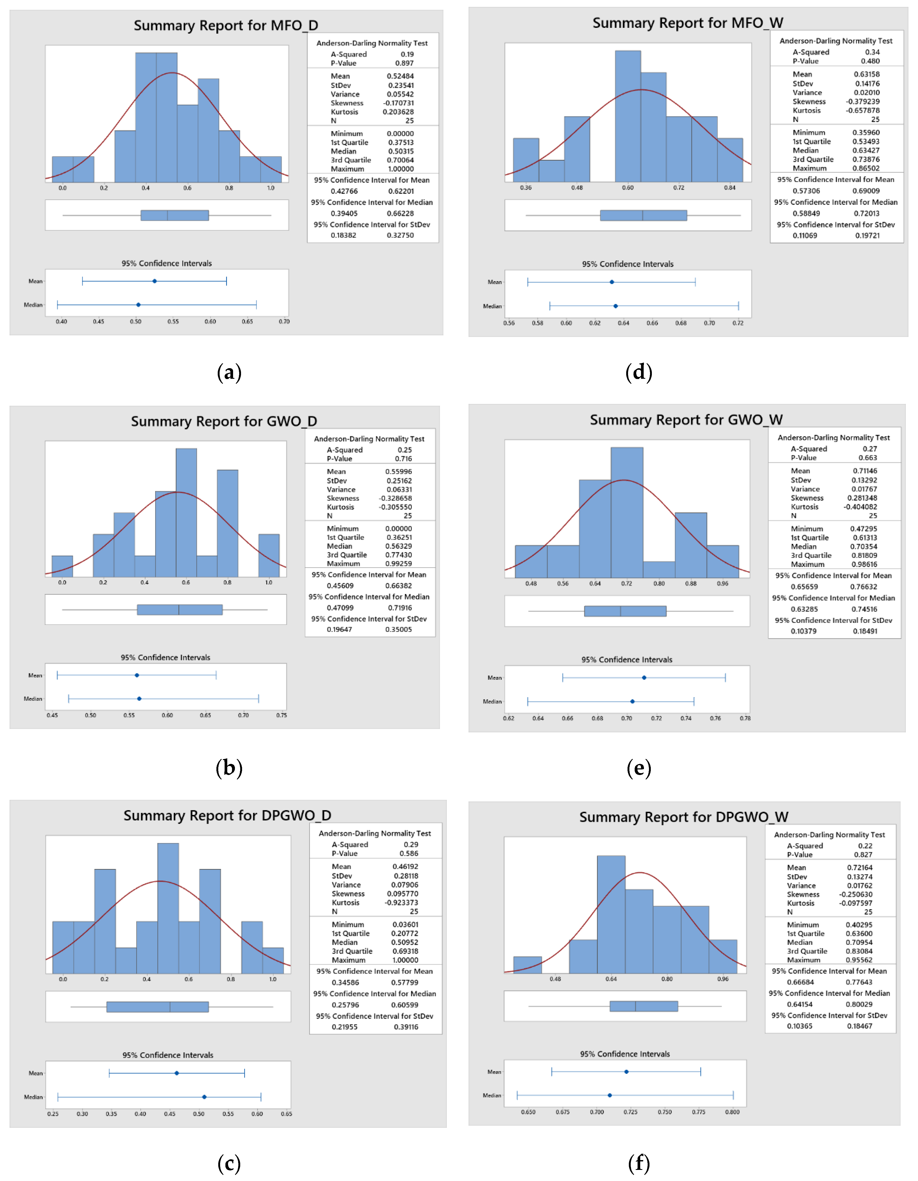
The implementation of DPGWO is presented as a flow chart in Figure 5. Python codes have been developed for all the algorithms and executed 25 times. The statistical analysis of the performance of the algorithm in terms of Deng’s value is presented in Figure 6.

The statistical analysis of output obtained using MFO, GWO, and DPGWO algorithms in terms of Deng’s value for both crack length training and testing data sets for 25 runs is shown in Figure 6. It is understood that the p-value shown in the summary report for all three algorithms will be above 0.005, which shows the output data obtained by the algorithms are normally distributed, hence the results are accepted. The p-value shown in Figure A4a–f confirmed that the results obtained by executing the Python codes for crack depth and width are acceptable.

4. Results and Discussion

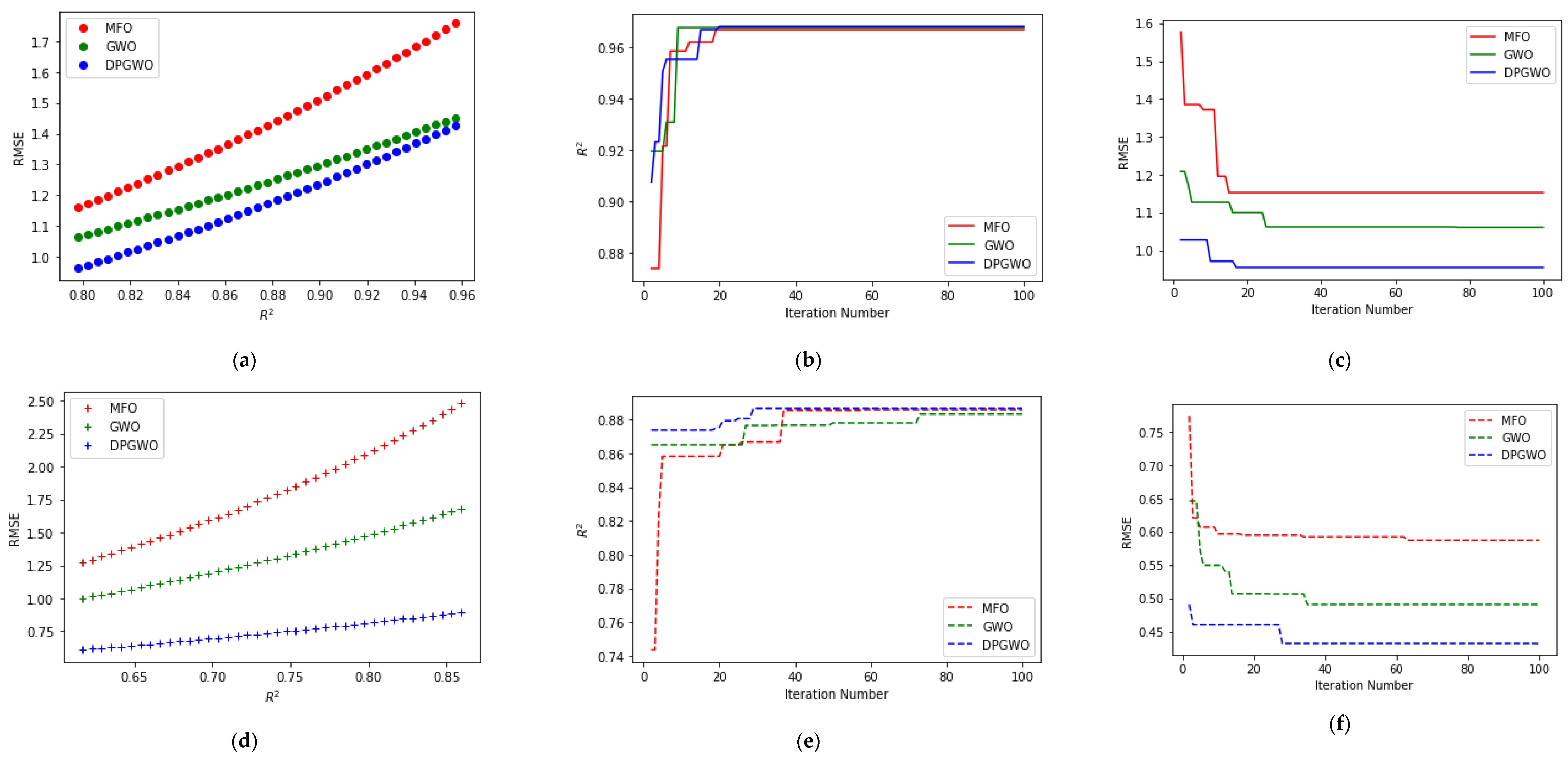
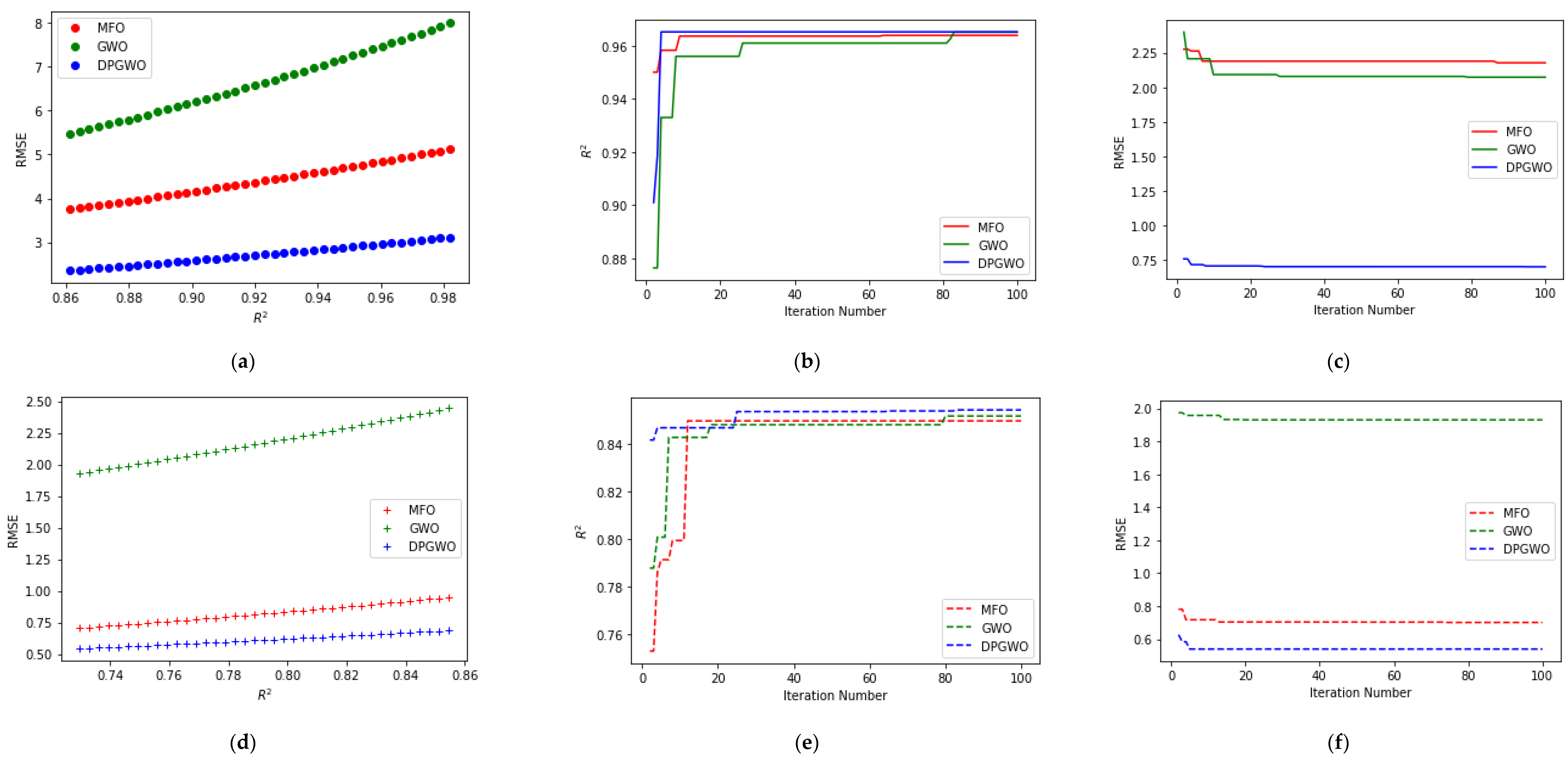
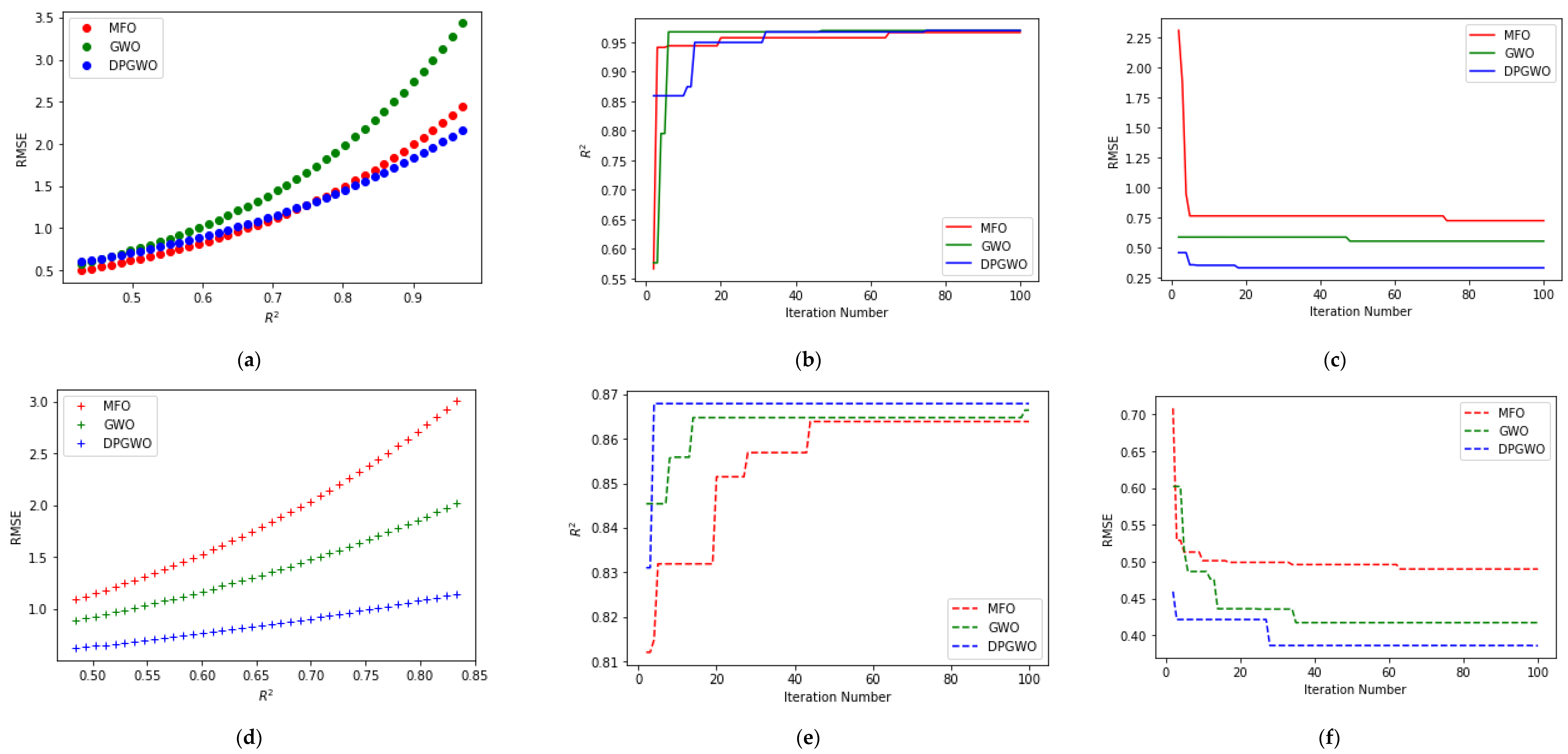
Figure 7a,d represent sample pareto solutions obtained using different algorithms for crack length training and testing data sets. It is understood that the solution obtained by implementing DPGWO is better than the solution obtained by other algorithms, namely MFO and GWO. Figure 7b,c,e,f depict the quick convergence of R² and RMSE in both training and testing data sets of crack length in DPGWO as compared with MFO and GWO. It is observed from Figure A5a,d that DPGWO has higher R² and lower RMSE values as compared with MFO and GWO in both cases of crack depth training and testing data sets. Early convergence is recorded in iteration numbers 16, 18, 30, and 28 in the cases of R²Tr, RMSETr, R²Tt, and RMSETt, respectively, in Figure A5b,c,e,f. Similar kinds of Pareto solution and convergence plots are obtained in the case of crack width, as shown in Figure A6a–f. It is also observed that a major difference in RMSE value is achieved in DPGWO as compared to MFO and GWO in Figure A6c,f. The p-value shown in Figure A4 confirms that the results obtained for 25 runs are normally distributed and acceptable. Performance indicators are used to compare the pareto solutions generated by the algorithms. In this work, two different performance indicators, namely inverted generational distance (IGD) and spacing (SP), are implemented to check the effectiveness of the algorithms. For problems with more than three objectives, IGD is used to measure the quality of pareto optimal solutions in terms of distribution and convergence, whereas SP is used to measure the distribution and spread of pareto optimal solutions. In both cases, the lower the value, the better the performance of the algorithm. From

Table 12. Performance Indicators of Algorithms [30].

Crack Dimension	Algorithm	IGD	SP
Crack Length	MFO	0.10066	0.05977
	GWO	0.10413	0.04707
	DPGWO	0.09652	0.04558
Crack Length	MFO	0.23810	0.49592
	GWO	0.21844	0.24535
	DPGWO	0.19339	0.08908
Crack Length	MFO	0.20932	0.15989
	GWO	0.34371	0.13514
	DPGWO	0.08245	0.06335

, it is confirmed that the DPGWO algorithm has lower values of IGD and SP as compared to the other two algorithms, hence it is outperformed.

To further support the performance of the algorithms, Friedman’s test, a non-parametric test, has been implemented in this work. This test is used to determine whether statistically significant differences exist between the means of three or more groups. In this work, the Deng’s values obtained by 25 runs using three algorithms are considered for ranking and the calculation of mean values. Using the “Friedman ()” function in Matlab, this test is conducted.

Table 13. Friedman’s Test Values and Mean Ranking of Algorithms [25].

Crack Dimensions	Mean Rank			Probability
	MFO	GWO	DPGWO
Crack Length	2.2	1.56	2.24	0.0263
Crack Depth	1.98	1.78	2.23	0.0049
Crack Width	1.84	2.04	2.12	0.0093

represents Friedman’s Test values and the mean ranking of each algorithm. All the probability values of crack dimensions are less than 0.05, which shows that the algorithm’s performance differs from each other, i.e., a significant effect will be there on the selection of algorithms. Usually, a lower value will be allotted rank 1 in Friedman’s Test. But in this work, the higher the Deng’s value, the better the solution; the higher the mean rank value, the higher the performance of the algorithm; hence, it is proved that the mean rank value of 2.24 in the case of crack length prediction using DPGWO outperformed as compared to the mean rank values of 2.2 and 1.56 of the MFO and GWO algorithms, respectively. Similarly, in the case of crack depth and width prediction, the mean rank of DPGWO will be 2.23 and 2.12, which are higher than the mean rank of MFO and GWO.

The number of features and their combinations obtained by implementing the MFO, GWO, and DPGWO for each crack dimension are presented in

Table 14. List of Features Considered in Various Methods.

FNo.	Fname	Crack Length					Crack Depth					Crack Width
		TM	DM	OT			TM	DM	OT			TM	DM	OT
				MFO	GWO	DPGWO			MFO	GWO	DPGWO			MFO	GWO	DPGWO
0	UNF											N		N	N
1	ETR	N	N		N	N	N		N		N
2	DSL								N			N	N	N	N
3	CST			N		N				N		N		N	N	N
4	ID			N	N				N	N		N	N			N
5	CN				N	N				N	N	N	N
6	H		N		N
7	AC			N		N	N	N	N		N			N		N
8	CS
9	CP
10	MP
11	SS
12	SA
13	SV
14	SE
15	DV
16	DE	N	N	N		N
17	IMC(1)									N	N				N	N
18	IMC(2)		N
19	MCC
20	INN		N
21	IDN	N		N	N		N		N	N	N			N	N	N
No. of Features		19	17	17	17	17	19	21	17	17	17	17	19	17	17	17

, along with features considered in the Taguchi Orthogonal Array Method (TM) and Desirability Method (DM). In Table 14, ‘N’ represents that the particular feature is not selected by the methods/algorithms.

The feature that has a higher count of ‘N’ is decided to be an important feature. The list of not-important features compared by various methods is presented in

Table 15. Not Importance Features.

FNo.	FName
1	ETR
3	CST
4	ID
7	AC
21	IDN

. A total of 5 out of 22 features are not considered important features.

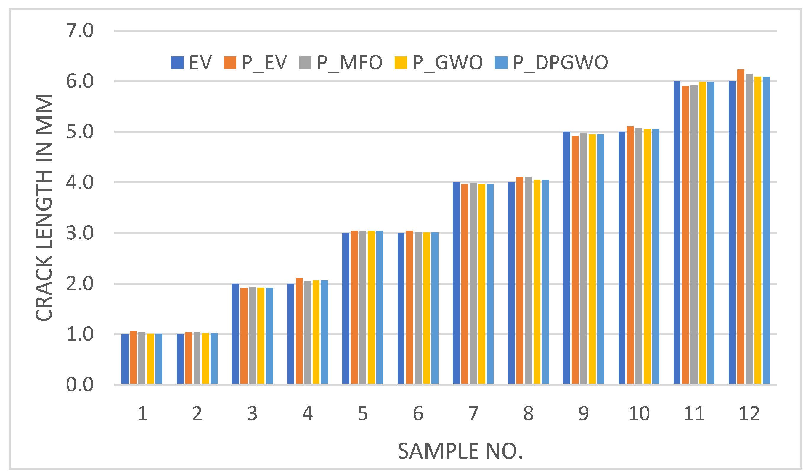
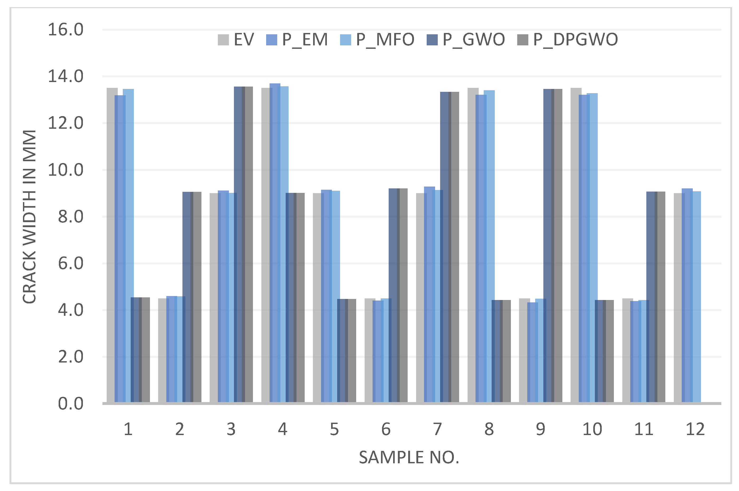
The performance metrics for the sample considered in the existing literature by Daniel et al. [12] are calculated based on the number of features and their combinations given in

Table 16. Comparison of Performance with existing and proposed algorithms.

Performance Metrics	EM	MFO	GWO	DPGWO
R2	0.9970	0.9987	0.9981	0.9992
	0.9938	0.9975	0.9966	0.9989
	0.9969	0.9993	0.9990	0.9994
RMSE	0.101	0.066	0.078	0.050
	0.032	0.020	0.023	0.014
	0.208	0.099	0.126	0.089
MAE	0.0872	0.0563	0.0568	0.0417
	0.0247	0.0147	0.0135	0.0099
	0.1922	0.0792	0.1028	0.0727
MAPE	2.93	1.88	1.60	1.38
	3.09	1.72	1.60	1.16
	2.25	0.91	1.09	0.91

. Figure 8, Figure 9 and Figure 10 represent the actual crack dimensions of the sample along with the calculated crack dimensions using the existing methods, MFO, GWO, and DPGWO. It is clear that all the dimensions calculated by DPGWO are very close to the actual dimensions. Table 16 represents the comparison of the performance metrics with existing and proposed algorithms for the sample data set considered by Daniel et al. It is observed that the R² value is higher in DPGWO as compared with the existing methods, MFO, and GWO. In the meantime, other metrics like RMSE, MAE, and MAPE are also lower in DPGWO as compared with others. It shows that the DPGWO performed well. The statistical comparison of computation time for the proposed DPGWO with MFO and GWO is shown in

Table 17. Comparison of computation time of algorithms.

Variable	Samples	Mean	StDev	Variance	Minimum	Q1	Median	Q3	Maximum	Skewness	Kurtosis
DPGWO	12	45	8.23	67.68	32.1	39.95	43.7	52.77	59.6	0.22	−0.65
GWO	12	38.4	6.98	48.75	29.6	31.62	39.25	41.38	51.8	0.57	−0.09
MFO	12	108.42	15.64	244.77	89.6	95.93	103.75	126	133.7	0.42	−1.36

. It is understood that the minimum computation times of DPGWO, MFO, and GWO will be 32.1 s, 29.6 s, and 89.6 s, respectively. Due to the introduction of life, reproduction, and disease strategies in DPGWO, the computation time is 8.4% higher than the GWO algorithm and 64.2% lower than the MFO algorithm.

5. Conclusions

In this work, the best ML model suitable to predict the crack dimensions from the given 22 GLCM features extracted from MFL images reported by Daniel et al. [12], was determined using the Taguchi L16 orthogonal array experimental design. Out of six ML models, the XGB model is identified as the best suited for the proposed problem. Apart from that, two-filter-based feature selection methods are implemented for prioritizing the features. The performance of the ML models is examined based on the number of features and their combinations. Meta-heuristic algorithms, namely MFO, GWO, and a new variant of GWO called DPGWO, are implemented to identify the number of features and their combinations to achieve better performance of the selected XGB ML model. The proposed method proved that by eliminating 23% of the number of features as compared with the existing method, it was possible to get good performance using the XGB ML model. Also, in this work, it is identified that the features ETR, CST, ID, AC, and IDN are not important features, i.e., these features are eliminated during the prediction of crack dimensions. The effectiveness of the proposed DPGWO is proved by comparing Friedman’s Test and performance indicators’ values, viz., IGD and SP with MFO and GWO. Also, the proposed method is implemented on the 12-test data set carried out by Daniel et al. [12]. As compared to the existing method, the proposed DPGWO performed well in calculating performance metrics like R², RMSE, MAE, and MAPE. Approximately 0.2 to 0.5% improvements in R² value, 50% to 57% improvement in RMSE value, 52% to 62% improvement in MAE value, and 53% to 63% improvement in MAPE values are reported by using a smaller number of features, i.e., 17 and its combinations, and implementing a new variant of GWO called DPGWO. As a further scope, the wrapper method of features selection along with the multi-regressor concept of ML models may be considered to improve performance. Apart from that, the crack dimensions may be changed from numerical to categorical data type, and ML classifiers can be introduced instead of ML regressors. The proposed DPGWO may be implemented for constrained engineering problems.

References

1. Gupta, M.; Khan, M.A.; Butola, R.; Singari, R.M. Advances in applications of Non-Destructive Testing (NDT): A Review. Adv. Mater. Process. Technol. 2021, 8, 2286–2307. [Google Scholar] [CrossRef]
2. Liu, C.; Peng, Z.; Cui, J.; Huang, X.; Li, Y.; Chen, W. Development of crack and damage in shield tunnel lining under seismic loading: Refined 3D finite element modeling and analyses. Thin-Walled Struct. 2023, 185, 110647. [Google Scholar] [CrossRef]
3. Gao, Z.; Hong, S.; Dang, C. An experimental investigation of subcooled pool boiling on downward-facing surfaces with microchannels. Appl. Therm. Eng. 2023, 226, 120283. [Google Scholar] [CrossRef]
4. Liu, H.; Yue, Y.; Liu, C.; Spencer, B.; Cui, J. Automatic recognition and localization of underground pipelines in GPR B-scans using a deep learning model. Tunn. Undergr. Space Technol. 2023, 134, 104861. [Google Scholar] [CrossRef]
5. Xia, Y.; Shi, M.; Zhang, C.; Wang, C.; Sang, X.; Liu, R.; Zhao, P.; An, G.; Fang, H. Analysis of flexural failure mechanism of ultraviolet cured-in-place-pipe materials for buried pipelines rehabilitation based on curing temperature monitoring. Eng. Fail. Anal. 2022, 14, 106763. [Google Scholar] [CrossRef]
6. Wang, Y.-Y.; Lou, M.; Wang, Y.; Wu, W.-G.; Yang, F. Stochastic Failure Analysis of Reinforced Thermoplastic Pipes Under Axial Loading and Internal Pressure. China Ocean Eng. 2022, 36, 614–628. [Google Scholar] [CrossRef]
7. Zeng, L.; Lv, T.; Chen, H.; Ma, T.; Fang, Z.; Shi, J. Flow accelerated corrosion of X65 steel gradual contraction pipe in high CO2 partial pressure environments. Arab. J. Chem. 2023, 16, 104935. [Google Scholar] [CrossRef]
8. Singh, W.S.; Rao, B.P.; Thirunavukkarasu, S.; Mahadevan, S.; Mukhopadhyay, C.; Jayakumar, T. Development of magnetic flux leakage technique for examination of steam generator tubes of prototype fast breeder reactor. Ann. Nucl. Energy 2015, 83, 57–64. [Google Scholar] [CrossRef]
9. Zhang, J.; Liu, X.; Xiao, J.; Yang, Z.; Wu, B.; He, C. A comparative study between magnetic field distortion and magnetic flux leakage techniques for surface defect shape reconstruction in steel plates. Sens. Actuators A Phys. 2019, 288, 10–20. [Google Scholar] [CrossRef]
10. Suresh, V.; Abudhahir, A.; Daniel, J. Development of magnetic flux leakage measuring system for detection of defect in small diameter steam generator tube. Measurement 2017, 95, 273–279. [Google Scholar] [CrossRef]
11. Suresh, V.; Abudhahir, A.; Daniel, J. Characterization of defects on ferromagnetic tubes using magnetic flux leakage. IEEE Trans. Magn. 2019, 55, 6200510. [Google Scholar] [CrossRef]
12. Daniel, J.; Abudhahir, A.; Paulin, J.J. Magnetic Flux Leakage (MFL) based defect characterization of steam generator tubes using artificial neural networks. J. Magn. 2017, 22, 34–42. [Google Scholar] [CrossRef] [Green Version]
13. Wang, W.; Kiik, M.; Peek, N.; Curcin, V.; Marshall, I.J.; Rudd, A.G.; Wang, Y.; Douiri, A.; Wolfe, C.D.; Bray, B. A systematic review of machine learning models for predicting outcomes of stroke with structured data. PLoS ONE 2020, 15, e0234722. [Google Scholar] [CrossRef]
14. Liu, M.; Gu, Q.; Yang, B.; Yin, Z.; Liu, S.; Yin, L.; Zheng, W. Kinematics Model Optimization Algorithm for Six Degrees of Freedom Parallel Platform. Appl. Sci. 2023, 13, 3082. [Google Scholar] [CrossRef]
15. Xie, L.; Zhu, Y.; Yin, M.; Wang, Z.; Ou, D.; Zheng, H.; Liu, H.; Yin, G. Self-feature-based point cloud registration method with a novel convolutional Siamese point net for optical measurement of blade profile. Mech. Syst. Signal Process. 2022, 178, 109243. [Google Scholar] [CrossRef]
16. Lu, H.; Zhu, Y.; Yin, M.; Yin, G.; Xie, L. Multimodal Fusion Convolutional Neural Network With Cross-Attention Mechanism for Internal Defect Detection of Magnetic Tile. IEEE Access 2022, 10, 60876–60886. [Google Scholar] [CrossRef]
17. Devi, R.M.; Premkumar, M.; Kiruthiga, G.; Sowmya, R. IGJO: An improved golden jackel optimization algorithm using local escaping operator for feature selection problems. Neural Process. Lett. 2023, 1–89. [Google Scholar] [CrossRef]
18. Qaraad, M.; Amjad, S.; Hussein, N.K.; Elhosseini, M.A. An innovative quadratic interpolation salp swarm-based local escape operator for large-scale global optimization problems and feature selection. Neural Comput. Appl. 2022, 34, 17663–17721. [Google Scholar] [CrossRef]
19. Houssein, E.H.; Saber, E.; Ali, A.A.; Wazery, Y.M. Centroid mutation-based Search and Rescue optimization algorithm for feature selection and classification. Expert Syst. Appl. 2022, 191, 116235. [Google Scholar] [CrossRef]
20. Ganesh, N.; Shankar, R.; Čep, R.; Chakraborty, S.; Kalita, K. Efficient feature selection using weighted superposition attraction optimization algorithm. Appl. Sci. 2023, 13, 3223. [Google Scholar] [CrossRef]
21. Hu, F.; Qiu, L.; Xiang, Y.; Wei, S.; Sun, H.; Hu, H.; Weng, X.; Mao, L.; Zeng, M. Spatial network and driving factors of low-carbon patent applications in China from a public health perspective. Front. Public Health 2023, 11, 1121860. [Google Scholar] [CrossRef]
22. Dai, X.; Xiao, Z.; Jiang, H.; Alazab, M.; Lui, J.C.S.; Min, G.; Dustdar, S.; Liu, J. Task Offloading for Cloud-Assisted Fog Computing With Dynamic Service Caching in Enterprise Management Systems. IEEE Trans. Ind. Inform. 2023, 19, 662–672. [Google Scholar] [CrossRef]
23. Priyadarshini, J.; Premalatha, M.; Čep, R.; Jayasudha, M.; Kalita, K. Analyzing Physics-Inspired Metaheuristic Algorithms in Feature Selection with K-Nearest-Neighbor. Appl. Sci. 2023, 13, 906. [Google Scholar] [CrossRef]
24. Mirjalili, S.; Mirjalili, S.M.; Lewis, A. Grey Wolf Optimizer. Adv. Eng. Softw. 2014, 69, 46–61. [Google Scholar] [CrossRef] [Green Version]
25. Mahalingam, S.K.; Nagarajan, L.; Velu, C.; Dharmaraj, V.K.; Salunkhe, S.; Hussein, H.M.A. An Evolutionary Algorithmic Approach for Improving the Success Rate of Selective Assembly through a Novel EAUB Method. Appl. Sci. 2022, 12, 8797. [Google Scholar] [CrossRef]
26. Deng, H. A similarity-based approach to ranking multicriteria alternatives. In Advanced Intelligent Computing Theories and Applications. With Aspects of Artificial Intelligence: Third International Conference on Intelligent Computing, ICIC 2007, Qingdao, China, 21–24 August 2007; Huang, D.S., Heutte, L., Loog, M., Eds.; Lecture Notes in Computer Science; Springer: Berlin/Heidelberg, Germany, 2007; Volume 4682, pp. 253–262. [Google Scholar]
27. Mirjalili, S.; Aljarah, I.; Mafarja, M.; Heidari, A.A.; Faris, H. Grey Wolf Optimizer: Theory, Literature Review, and Application in Computational Fluid Dynamics Problems. In Nature-Inspired Optimizers; Springer: Cham, Switzerland, 2019; pp. 87–105. [Google Scholar] [CrossRef]
28. Arivalagan, S.; Sappani, R.; Čep, R.; Kumar, M.S. Optimization and Experimental Investigation of 3D Printed Micro Wind Turbine Blade Made of PLA Material. Materials 2023, 16, 2508. [Google Scholar] [CrossRef]
29. Saremi, S.; Mirjalili, S.Z.; Mirjalili, S.M. Evolutionary population dynamics and grey wolf optimizer. Neural Comput. Appl. 2015, 26, 1257–1263. [Google Scholar] [CrossRef]
30. Khalilpourazari, S.; Naderi, B.; Khalilpourazary, S. Multi-Objective Stochastic Fractal Search: A Powerful Algorithm for Solving Complex Multi-Objective Optimization Problems. Soft Comput. 2019, 24, 3037–3066. [Google Scholar] [CrossRef]
Figure 1. Proposed Methodology.
Applsci 13 08206 g001
Figure 2. Prioritized features for crack dimensions. (a) F Score-based prioritized features for Crack Length. (b) MIS-based prioritized features for Crack Length. (c) F Score-based prioritized Features for Crack Depth. (d) MIS-based prioritized features for Crack Depth. (e) F Score-based prioritized Features for Crack Width. (f) MIS-based prioritized features for Crack Width.
Applsci 13 08206 g002aApplsci 13 08206 g002b
Figure 3. Probability Plot of Performance Measures of ML Models in Crack Length. (a) Probability Plot for Crack Length-R2Tr. (b) Probability Plot for Crack Length-R2Tt. (c) Probability Plot for Crack Length-RMSETr. (d) Probability Plot for Crack Length-RMSETt.
Applsci 13 08206 g003aApplsci 13 08206 g003b
Figure 4. Factorial and Interaction Plots for Performance of ML Models for Crack Length Prediction. (a) R2 Factorial Plot for Training Dataset—L. (b) R2 Factorial Plot for Testing Dataset—L. (c) RMSEFactorial Plot for Training Dataset—L. (d) RMSEFactorial Plot for Testing Dataset—L. (e) R2 Interaction Plot for Training Dataset—L. (f) R2 Interaction Plot for Testing Dataset—L. (g) RMSE Interaction Plot for Training Dataset—L. (h) RMSE Interaction Plot for Testing Dataset—L.
Applsci 13 08206 g004aApplsci 13 08206 g004b
Figure 5. Implementation of DPGWO.
Applsci 13 08206 g005
Figure 6. Statistical Analysis of Output using different algorithms for Crack Length. (a) Statistical analysis of output using MFO for Crack Length. (b) Statistical analysis of output using GWO for Crack Length. (c) Statistical analysis of output using DPGWO for Crack Length.
Applsci 13 08206 g006
Figure 7. Pareto and Convergence Plot for Crack Length. (a) Pareto Plot for Training Data Set—Crack Length. (b) R2 Convergence Plot for Training Data Set—Crack Length. (c) RMSE Convergence Plot for Training Data Set—Crack Length. (d) Pareto Plot for Testing Data Set—Crack Length. (e) R2 Convergence Plot for Testing Data Set—Crack Length. (f) RMSE Convergence Plot for Testing Data Set—Crack Length.
Applsci 13 08206 g007
Figure 8. Experimental VS Predicted Value of Crack Length Using Different Algorithms (EV-Experimental Value; P_EM-Predicted value using the existing method; P_MFO, P_GWO and P_DPGWO-Predicted values based on the number of features and its combination obtained using MFO, GWO, and DPGWO algorithms.
Applsci 13 08206 g008
Figure 9. Experimental VS Predicted Value of Crack Depth Using Different Algorithms.
Applsci 13 08206 g009
Figure 10. Experimental VS Predicted Value of Crack Width Using Different Algorithms.
Applsci 13 08206 g010