Abstract
In this paper, a hybrid particle swarm optimization genetic algorithm LQR controller is used on a quarter car model with an active suspension system. The proposed control algorithm is utilized to overcome the shortcoming that the weight matrix Q and matrix R determined by experience in the traditional LQR control method. The proposed hybrid control method makes it possible to achieve the optimal control effect. A full-order state observer is proposed to observe the state of active suspension. A quarter car active suspension model and road input model are presented at first, and the LQR controller based on the hybrid particle swarm optimization genetic algorithm is utilized in the active suspension system control. Sprung mass acceleration, suspension deflection, and tire dynamic load are selected as the control effect evaluation index. Next, simulation results are presented. According to the results, compared with the passive suspension and active suspension with a traditional LQR control, there is an obvious reduction in the sprung mass acceleration, deflection, and tire dynamic load with an optimized controller under case 1 and case 2. Simultaneously, the system state fed back by the full-order state observer can effectively reflect the true state of the active suspension system.
1. Introduction
Vehicle suspension systems are the entire support systems consisting of springs and dampers between the car body and tires, and play a major role in modern vehicles. Suspension systems can isolate the vibrations created by road surfaces, which guarantee ride comfort and handling stability [1,2,3].
Generally speaking, according to the forms of damper, vehicle suspension systems are divided into three categories: passive suspension systems, semi-active suspension systems, and active suspension systems [4,5]. The passive suspension systems are assembled with irrevocable dampers. Semi-active suspension systems are constructed with various dampers. Thus, the passive suspension and semi-active suspension are not able to change with road conditions, and, they are limited in improving the performance of ride comfort and handling stability [6]. Compared with the passive and semi-active suspension, pneumatic or hydraulic actuators replace the dampers in active suspension systems, which can proactively generate the force to absorb and deliver the load produced by vehicle vibration [7]. Hence, active suspension systems possess better performance in ride comfort and road holding capability.
Due to the excellent characteristics of active suspension, many control algorithms were applied in active suspension controllers during the past few decades [8,9,10,11,12,13,14,15,16]. Su-Juan et al. [8] proposed a time-delay feedback controller to reduce suspension vibration. Williams et al. [9] carried out the sliding mode control in active suspension systems with data acquisition delay. Zheng Chao et al. [10] applied the integrated fuzzy wheelbase preview control to heavy-duty vehicles. In addition, many advanced control methods have attracted considerable interest, such as adaptive control, fuzzy logic control, NN control, and artificial intelligence, which have been studied by many scholars [11,12,13]. Recently, the model predictive control (MPC) attracted many scholars, drawing attention to vehicle control [14,15,16]. MPC is an optimization-based control method whose objective function uses relative errors [17].
In recent years, the linear quadratic regulator (LQR) control strategy received increasing attention, as it can easily realize the closed-loop control [18,19,20,21,22]. Compared with other control methods, LQR has a simple mathematical treatment and easily constructs objective function. The performance indexes of LQR are explicit physical parameters (for example, sprung mass acceleration, the deflection used in this paper). LQR is also a multi-objective optimization algorithm that can achieve the overall optimality. Moreover, it is easy to realize closed-loop control; thus, it is widely used in the vibration system [23,24]. At the same time, the LQR control method is one of the most important issues in active suspension control theory and is widely used.
LQR control is a control algorithm that faces multiple objectives, which can make the system’s comprehensive performance work the best. Ref. [18] proposed the LQR-based power train control method for fuel cell hybrid vehicles. Ref. [19] investigated the LQR controller for the carlike robot. Ref. [20] used the PID-LQR control method to improve vehicle ride comfort.
The key to the LQR control method lies in the selection of the weight matrices Q and R. Therefore, different approaches have arisen for the optimization of the weight matrix of the controller. However, there exists a shortcoming in the LQR control system, in which the weight coefficients of matrix Q and matrix R are determined by experience, which cannot guarantee the optimal performance. The traditional method can only rely on empirical selection, and the process is too cumbersome; it could not obtain the optimal solution [25,26,27]. Currently, the most commonly used methods include Genetic Algorithm (GA) and Particle Swarm Optimization (PSO). Recent studies have also mentioned an artificial fish algorithm.
GA has better converge performance, and can expand the search space to avoid falling into local solutions. According to the research in [22], to optimize the weight matrixes, the GA was successfully used in LQR control for active suspension. However, in the optimization based on GA, the search speed is slow and the robustness is poor and prone to produce early convergence [25].
To overcome the weak points of the LQR control, ref. [21] applied the PSO algorithm to optimize the weight coefficients of matrix Q and matrix R. PSO is computationally fast, simpler, more efficient, and converges easily compared with other algorithms [26]. However, this method is prone to falling into local optima [28]. The artificial fish algorithm is essentially similar to PSO, an optimization algorithm that simulates animal predation [27].
As a result, in this paper, a hybrid particle swarm optimization genetic algorithm is applied to optimize the LQR controller. The optimization method proposed in this paper fully considers the computational speed of PSO and the global search capability of GA. Therefore, the optimization method proposed in this paper has both optimization speed and global search capabilities.
In the active suspension systems control, the dynamics of the suspension system should be collected in real-time; however, the installation of a large number of sensors will not only affect the cost of the vehicle, but will also reduce the stability of the vehicle control system [29]. Therefore, this paper constructs a full-order state observer to observe the condition of the active suspension.
The main contributions of this paper are as follows: The random road input model and quarter car suspension model are established. A hybrid optimization algorithm that combines the advantages of the particle swarm optimization and genetic algorithm is used to optimize the weight matrix Q and matrix R in the LQR control. Moreover, the new controller is applied to the active suspension system. A full-order state observer is designed to observe the state of the active suspension. The simulation analysis of the active suspension system under case 1 and case 2 is carried out, and, lastly, the conclusion based on the data is presented.
2. System Model
2.1. Random Road Input Model
The car will generate vibration when driving on rough roads; thus, the suspension systems are designed to stabilize the body movement and improve the performance of the vehicle. In order to investigate the active suspension and control strategy, the input road model variables of the suspension system should be considered at first. The common road model in actual vehicle traffic can be divided into two categories: the random model and impact model.
Random uneven pavement is the most common road model in vehicle dynamics simulations, and also a common pavement in actual vehicle driving. Uneven pavement can be classified into several classes according to the roughness and unevenness of the pavement. According to the international standard ISO/TC108/SC2N67, the power spectral density function can be used to fit the simulation of pavement unevenness.
In this paper, the integration of white noise signals is used as the random road input model. The expression of the random road input model [30] is shown as:
where is the road displacement; is the random white noise signal; represents the low cut-off frequency; stands for the road roughness; v is the speed in simulation. In this paper, two cases are considered: in case 1: 80 km/h, m; in case 2: 60 km/h, m. The random road input of case 1 and case 2 are presented as Figure 1 and Figure 2.
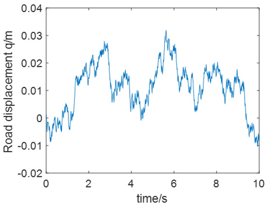
Figure 1.
The Random Road Input of Case 1.
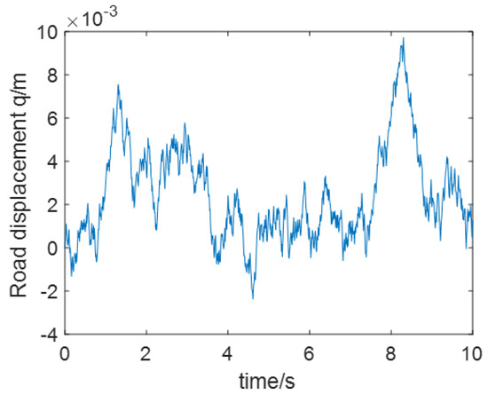
Figure 2.
The Random Road Input of Case 2.
2.2. Active Suspension Model
In this paper, a two-DOF quarter active suspension system model [31] is considered. Moreover, the model in this paper is shown in Figure 3. It assumed that the tire always keeps contact with the road.
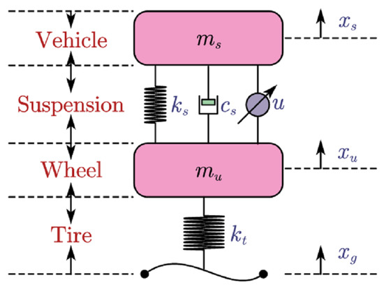
Figure 3.
The Quarter Car Active Suspension System.
In this model, and are the mass of sprung and un-sprung; and represent the displacement of the corresponding masses; and represent the stiffness of the vehicle suspension system and tire; denotes the active control force; is the damper coefficient.
Therefore, the dynamic mathematical model of a quarter car is as follows.
Define the following state variable. is the suspension dynamic deflection: represents the sprung mass velocity; denotes the tire deflection; is the velocity of the un-sprung mass; is selected as the disturbance input caused by road roughness.
The state vector is expressed as follows.
Define the following output state variables, which are selected as follows.
Therefore, the dynamical equation can be written in the following state space form.
where , , , , , , .
3. Controller Design
3.1. LQR Controller Design
The linear quadratic regulator (LQR) control strategy takes the objective function as the object [32,33]. Generally, the suspension dynamic deflection and vertical acceleration of the sprung mass are used to evaluate the performance of ride comfort; the tire dynamic load is usually used to evaluate the performance of the vehicle handling stability. Therefore, the LQR control objective function can be expressed as
where , , , and represent the weight coefficients of the LQR control objective function. According to the traditional empirical method, it can be determined that , , and . As active force is not involved in performance indicators, .
When rewriting the objective function, a linear quadratic regulator matrix form is shown as
where is the weight matrix of the stable variable; is the weight matrix of the control variable.
Then, bringing into the equation of the linear quadratic regulator matrix form yields:
where , , .
Therefore, Equation (8) can be expressed as (9).
In the LQR controller design, the control law can be expressed as (10).
where is the output feedback gain matrix. Moreover, P can be obtained by solving the Riccati equation.
Let . , , , and are the coefficients of the control load equation.
According to (5), the state space form of the quarter car active suspension with LQR is shown as (12).
where
3.2. LQR Controller with Hybrid Algorithm
In this paper, a hybrid particle swarm optimization genetic algorithm is used to find the optimal weight coefficient. The genetic algorithm has more excellent convergence compared with other traditional optimization algorithms. However, the ability of the local search convergence is poor, which causes the low efficiency. Meanwhile, the particle swarm optimization algorithm operates efficiently. Thus, in this paper, a hybrid optimization algorithm that combines the advantages of these two algorithms is used to find the optimal solution. The particle swarm optimization genetic hybrid algorithm flow chart is shown in Figure 4.
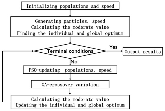
Figure 4.
Hybrid Particle Swarm Optimization Genetic Algorithm Flow Chart.
We select sprung mass acceleration, suspension deflection, and tire dynamic load as performance indicators. However, for the inconsistent units and orders of magnitude, the performance indicators selected need to be normalized. Therefore, the fitness function is given by
where: , and are the root mean square values of the sprung mass acceleration, sprung mass deflection, and tire load under control. , , and are the root mean square values of the sprung mass acceleration, sprung mass deflection, and tire load without control. The constraints are denoted as (14).
The optimization process of the LQR control with the hybrid particle swarm optimization genetic algorithm is shown in Figure 5.
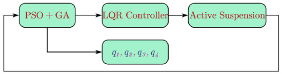
Figure 5.
LQR Control with Particle Swarm Optimization Genetic Hybrid Algorithm Flow Chart.
3.3. Full-Order Observer Design
Constructing the state observer according to the input variables and output variables; therefore, the mathematical model of the full-order state observer [34] can be obtained as (15).
where: is the system state estimation vector. L is the gain matrix of the observer. According to (12) and (15), the state error dynamic equation can be expressed as (16).
After simplification, (17) is obtained.
Solving the equation yields:
is the system matrix of the observer. The key to the observer design is whether can always be guaranteed under any initial conditions. In other words, if the eigenvalues of are arbitrarily configurable, and the eigenvalues of the matrix could be properly configured, then the state of the observer would quickly approach the state of the system.
A sufficient necessary condition for all poles of the system or eigenvalues that are arbitrarily configurable is that is fully controllable. In other words, the eigenvalues of the matrix have negative real parts, or .
In the control system proposed in this paper, matrix can be obtained, and . Thus, the control system proposed is observable, and poles of the system are arbitrarily configurable.
For systems with arbitrary configurations of poles, different poles affect the time for the observer to stabilize, but have no effect on the final state of the observer [35].
However, when all the real parts of the eigenvalues are strictly negative, then the system is stable.
Let eigenvalues . . The characteristic equation of the observer can be expressed as follows.
Then. and can be obtained. Therefore, the mathematical model of the full-order state observer can be obtained.
4. Simulation Analysis and Comparison
The detailed simulations results are presented in this section to verify the efficacy of the proposed control method. To illustrate the performance of the controller proposed in this paper, the simulation is carried out based on passive suspension, active suspension with traditional LQR control, active suspension with optimization LQR control, and the full-order state observer under case 1 and case 2. To evaluate the performance of suspension systems, the sprung mass acceleration, sprung mass deflection, and tire dynamic load are selected as evaluation indicators. The smaller the value of sprung mass acceleration and deflection, the better the performance of the ride comfort of the suspension system. The lower the value of the tire dynamic load, the better the performance of the road holding. The closer to zero the value of the observer estimation error is, the better the observer.
The vehicle parameters [36] used for simulation in this paper are shown in Table 1.

Table 1.
Paremeters of Suspension System.
The simulation results under case 1 are shown in Figure 6, Figure 7 and Figure 8. The simulation results under case 2 are shown in Figure 9, Figure 10 and Figure 11. Statistical results of simulation data are shown as Figure 12, Figure 13 and Figure 14 and Table 2 and Table 3.
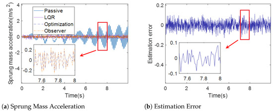
Figure 6.
Sprung Mass Acceleration (case 1).
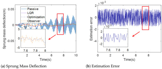
Figure 7.
Sprung Mass Defllection (case 1).
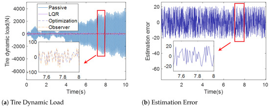
Figure 8.
Tire Dynamic Load (case 1).
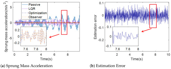
Figure 9.
Sprung Mass Acceleration (case 2).
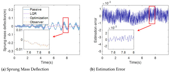
Figure 10.
Sprung Mass Deflection (case 2).
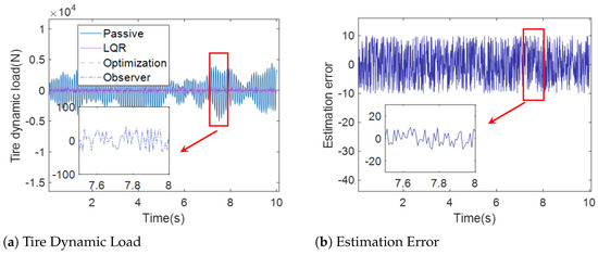
Figure 11.
Tire Dynamic Load (case 2).
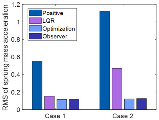
Figure 12.
RMS of Sprung Mass Acceleration.
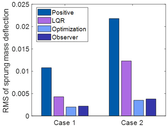
Figure 13.
RMS of Sprung Mass Deflection.
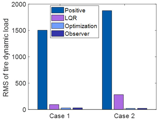
Figure 14.
RMS of Tire Dynamic Load.
Table 2.
Comparison of RMS values in case 1.
Table 3.
Comparison of RMS values in case 2.
Figure 6a, Figure 7a and Figure 8a demonstrate the sprung mass acceleration, deflection, tire dynamic load of passive suspension, active suspension with traditional LQR control, active suspension with optimization LQR, and the full-order state observer under case 1. Figure 6b, Figure 7b and Figure 8b show the estimation error of the sprung mass acceleration, deflection, and tire dynamic load under case 1.
Figure 9a, Figure 10a and Figure 11a show the sprung mass acceleration, deflection, tire dynamic load of passive suspension, active suspension with traditional LQR control, active suspension with optimization LQR, and the full-order state observer under case 2. Figure 9b, Figure 10b and Figure 11b show the estimation error of the sprung mass acceleration, deflection, and tire dynamic load under case 2.
Figure 12, Figure 13 and Figure 14 and Table 2 and Table 3 show the statistical results of the RMS of the sprung mass acceleration, RMS of the sprung mass deflection, and RMS of the tire dynamic load under each state.
Figure 6a and Figure 9a show the sprung mass acceleration for passive suspension, active suspension with traditional LQR control, active suspension with optimization LQR control, and the full-order state observer under case 1 and case 2. It can be observed from Figure 6a and Figure 9a that the curve of the sprung mass acceleration under active suspension with the optimization LQR control is smoother than the curve of the passive suspension, active suspension with traditional LQR control, and active suspension, indicating that the ride comfort under the active suspension with optimization LQR control is better than the other cases.
In Figure 7a and Figure 10a, the sprung mass deflection for passive suspension, active suspension with traditional LQR control, active suspension with optimization LQR control, and the full-order state observer under case 1 and case 2 are shown. It can be observed from Figure 7a and Figure 10a that the curve of the sprung mass deflection under active suspension with optimization LQR control is less pronounced than the curve of the passive suspension, active suspension with traditional LQR control, and active suspension, suggesting that the active suspension with the optimization LQR control performs better in terms of road holding than the other cases.
Figure 8a and Figure 11a show the tire dynamic load curve of the passive suspension, active suspension with traditional LQR control, active suspension with optimization LQR control, and the full-order state observer under case 1 and case 2. Moreover, it can be observed from Figure 8a and Figure 11a that the curve of the tire dynamic load under active suspension with the optimization LQR control is smaller than the curve of the passive suspension, active suspension with traditional LQR control, and active suspension, which illustrates that the capability of active suspension under optimization LQR control is more stable over the other methods.
In Figure 6b and Figure 8b, the estimation error of the full-order state observer with the sprung mass acceleration, sprung mass deflection, and tire dynamic load under case 1 is presented. Moreover, Figure 9b and Figure 11b show the estimation error of the full-order state observer with the sprung mass acceleration, sprung mass deflection, and tire dynamic load under case 2. It is obvious that the estimation error of the full-order state observer is too small, which influences the accuracy of the estimation. The output of the observer provides a satisfactory indication of the state of the system.
From Figure 12, Figure 13 and Figure 14 and Table 2 and Table 3, it can be observed that the RMS of the sprung mass acceleration, deflection, and tire dynamic load under LQR control with optimization decrease by , , in case 1, , , and in case 2 compared with the LQR control without optimization.
According to the above results, the sprung mass acceleration, sprung mass deflection, and tire dynamic load under the optimization LQR control method are obviously reduced, and the vibration of the suspension system is effectively suppressed compared with the other suspension systems; thus, the ride comfort and handling stability are ensured. Moreover, this illustrates that the suspension system can effectively maintain its own stability under the condition of receiving external disturbances. Therefore, the proposed controller in this paper can reduce suspension deflection and acceleration to a great extent, further demonstrating the viability of the proposed control method. Simultaneously, the system state fed back by the full-order state observer can effectively reflect the true state of the active suspension system. The hybrid control algorithm could overcome the shortcoming existing in the conventional LQR control.
5. Conclusions
This paper mainly discusses an improved optimization of the LQR control method that adapts the hybrid particle swarm optimization and genetic algorithm for active suspension. The controller for the active suspension is crucial for effectively improving the performance in the ride comfort and handling stability of active suspension systems. However, there are unavoidable flaws, in which weight coefficients of matrix Q and matrix R are determined by experience in the traditonal LQR control method for an active suspension that cannot obtain the optimal result. Hence, the traditional LQR controller for active suspension is imprecise and unperfect. Based on these shortcomings, in this paper, an improved optimization LQR control method that adapts the hybrid particle swarm optimization and genetic algorithm is presented, and then this controller is applied to the active suspension to overcome these limitations.
The quarter car suspension model and road input model are considered at first. Then, the hybrid controller is conducted. After that, a simulation is conducted within a Matlab Simulink environment. Finally, the performance of the proposed controller in this paper is compared with the passive suspension and active suspension under the traditional LQR control. Moreover, a full-order state observer is designed to feedback on the state of the suspension system.
The simulation based on the random road input model, quarter car suspension model, passive suspension, LQR controller, and optimization controller is conducted. From the simulation results, it is confirmed that the sprung mass vibration and deflection are well reduced, which are regarded as important characteristics to evaluate the performance of ride comfort. The tire dynamic load used to evaluate the performance of the road holding is restrained.
Thus, all of the above simulation results provide a foundation, with which the control method proposed in this paper can significantly improve the performance of ride comfort and road holding stability. On the one hand, the proposed hybrid control algorithm in this paper can overcome the limitation of the traditional LQR controller for active suspenson. On the other hand, the proposed controller is efficient and very promising in order to guarantee the performance of the active suspension.
Moreover, this paper also applies the full-order state observer to monitor the state of the active suspension system. The simulation results indicate that the observer can effectively reflect the true state of the active suspension system.
The experimental validation is an important part of the conducted research and is better for revealing the application in real suspension systems. However, our current study is limited in experimental conditions, and relevant research could not help to conduct the experiments. Thus, our future research will focus more on the experimental validation of controllers and mainly include the following points. First, we hope to apply the proposed control method to the nonlinear active suspension, which is more precise for a real suspension model. Second, we hope to establish an adaptive controller for a full car active suspension dynamic model and apply it to real suspension.
Author Contributions
Methodology, W.Z.; Writing—original draft, W.Z.; Writing—review & editing, L.G.; Supervision, L.G. All authors have read and agreed to the published version of the manuscript.
Funding
This research received no external funding.
Acknowledgments
The authors appreciate the support from Liang Gu and the editor and the reviewers for their constructive comments.
Conflicts of Interest
The authors declare no conflict of interest.
References
- Du, H.; Zhang, N.; Lam, J. Parameter-dependent input-delayed control of uncertain vehicle suspensions. J. Sound Vib. 2008, 317, 537–556. [Google Scholar] [CrossRef]
- Marzbanrad, J.; Ahmadi, G.; Zohoor, H.; Hojjat, Y. Stochastic optimal preview control of a vehicle suspension. J. Sound Vib. 2004, 275, 973–990. [Google Scholar] [CrossRef]
- Gohrle, C.; Schindler, A.; Wagner, A.; Sawodny, O. Design and Vehicle Implementation of Preview Active Suspension Controllers. Control Syst. Technol. 2014, 22, 1135–1142. [Google Scholar] [CrossRef]
- Priyandoko, G.; Mailah, M.; Jamaluddin, H. Vehicle active suspension system using skyhook adaptive neuro active force control. Mech. Syst. Signal Process. 2009, 23, 855–868. [Google Scholar] [CrossRef]
- Hasbullah, F.; Faris, W.F.; Darsivan, F.J.; Abdelrahman, M. Ride comfort performance of a non-linear full-car using active suspension system with active disturbance rejection control and input decoupling transformation. Int. J. Heavy Veh. Syst. 2019, 26, 188–224. [Google Scholar] [CrossRef]
- Kazemipour, A.; Novinzadeh, A.B. Adaptive fault-tolerant control for active suspension systems based on the terminal sliding mode approach. Proc. Inst. Mech. Eng. Part C J. Mech. Eng. Sci. 2020, 234, 501–511. [Google Scholar] [CrossRef]
- Liu, B.; Saif, M.; Fan, H. Adaptive Fault Tolerant Control of a Half-Car Active Suspension Systems Subject to Random Actuator Failures. IEEE/ASME Trans. Mechatron. 2016, 21, 2847–2857. [Google Scholar] [CrossRef]
- Shao, S.J.; Jing, D.; Ren, C.B. Multiobjective Optimization of Nonlinear Active Suspension System with Time-Delayed Feedback. Math. Probl. Eng. 2020, 2020, 9526359. [Google Scholar] [CrossRef]
- Alves, U.; Garcia, J.; Teixeira, M.; Garcia, S.C.; Rodrigues, F.B. Sliding Mode Control for Active Suspension System with Data Acquisition Delay. Math. Probl. Eng. 2014, 2014, 529293. [Google Scholar] [CrossRef]
- Xie, Z.; Wong, P.K.; Jing, Z.; Tao, X.; Wong, K.I.; Hang, C.W. A Noise-Insensitive Semi-Active Air Suspension for Heavy-Duty Vehicles with an Integrated Fuzzy-Wheelbase Preview Control. Math. Probl. Eng. 2013, 2013, 121953. [Google Scholar] [CrossRef]
- Foda, S.G. Fuzzy control of a quarter-car suspension system. In Proceedings of the 12th International Conference on Microelectronics (IEEE Cat. No.00EX453), Tehran, Iran, 31 October–2 November 2000; pp. 231–234. [Google Scholar]
- Al-Holou, N.; Lahdhiri, T.; Joo, D.S.; Weaver, J.; Al-Abbas, F. Sliding mode neural network inference fuzzy logic control for active suspension systems. IEEE Trans. Fuzzy Syst. 2002, 10, 234–246. [Google Scholar] [CrossRef]
- Herrnberger, M.; Lohmann, B. Nonlinear Control Design for an Active Suspension Using Velocity-Based Linearisations. IFAC Proc. Vol. 2010, 43, 330–335. [Google Scholar] [CrossRef]
- Falcone, P.; Borrelli, F.; Asgari, J.; Tseng, H.E.; Hrovat, D. Predictive Active Steering Control for Autonomous Vehicle Systems. IEEE Trans. Control Syst. Technol. 2007, 15, 566–580. [Google Scholar] [CrossRef]
- Gutjahr, B.; Gröll, L.; Werling, M. Lateral Vehicle Trajectory Optimization Using Constrained Linear Time-Varying MPC. IEEE Trans. Intell. Transp. Syst. 2017, 18, 1586–1595. [Google Scholar] [CrossRef]
- Raimondo, D.M.; Limon, D.; Lazar, M.; Magni, L.; Camacho, E.F. Min-max Model Predictive Control of Nonlinear Systems: A Unifying Overview on Stability. Eur. J. Control 2009, 15, 5–21. [Google Scholar] [CrossRef]
- Gulbudak, O.; Gokdag, M. Finite control set model predictive control approach of nine switch inverter-based drive systems: Design, analysis, and validation. ISA Trans. 2020, 110, 283–304. [Google Scholar] [CrossRef]
- Yun, H.; Zhao, Y.; Liu, Z.; Hao, K. LQR-Based Power Train Control Method Design for Fuel Cell Hybrid Vehicle. Math. Probl. Eng. 2013, 2013, 968203. [Google Scholar]
- Lin, F.; Lin, Z.; Qiu, X. LQR controller for car-like robot. In Proceedings of the 2016 35th Chinese Control Conference (CCC), Chengdu, China, 27–29 July 2016; pp. 2515–2518. [Google Scholar]
- Deng, Z.; Shi, B.; Wei, D.; Wang, S. Research on Energy Reclaiming Active Suspension Control Strategy Based on Linear Motor and Hydraulic Hybrid System. J. Phys. Conf. Ser. 2021, 1910, 012041. [Google Scholar] [CrossRef]
- Fang, J. The LQR Controller Design of Two-Wheeled Self-Balancing Robot Based on the Particle Swarm Optimization Algorithm. Math. Probl. Eng. 2014, 2014, 729095. [Google Scholar] [CrossRef]
- Zhang, J.; Xu, Z.; Gao, R.; Han, W. Studying of fuzzy logic control semi-active suspension based on improved genetic algorithm. Adv. Mater. Res. 2010, 143–144, 956–960. [Google Scholar] [CrossRef]
- Ghaffarzadeh, H.; Younespour, A. Active Tendons Control of Structures Using Block Pulse Functions. Struct. Control Health Monit. 2015, 21, 1453–1464. [Google Scholar] [CrossRef]
- Ambrosio, P. An optimal vibration control logic for minimising fatigue damage in flexible structures. J. Sound Vib. 2014, 333, 1269–1280. [Google Scholar] [CrossRef]
- Mohammed, I.K.; Abdulla, A.I. Elevation, pitch and travel axis stabilization of 3DOF helicopter with hybrid control system by GA-LQR based PID controller. Int. J. Electr. Comput. Eng. 2020, 10, 1868–1878. [Google Scholar] [CrossRef]
- Kumar, E.V.; Raaja, G.S.; Jerome, J. Adaptive PSO for optimal LQR tracking control of 2 DoF laboratory helicopter. Appl. Soft Comput. 2016, 41, 77–90. [Google Scholar] [CrossRef]
- Wang, L.; Tan, P.; Li, S.-P. Optimal analysis of weight matrices of LQR algorithm for stochastic structure-AMD system based on artificial fish algorithm. J. Vib. Shock 2016, 35, 154–158. [Google Scholar]
- Kao, Y.T.; Zahara, E. A hybrid genetic algorithm and particle swarm optimization for multimodal functions. Appl. Soft Comput. 2008, 8, 849–857. [Google Scholar] [CrossRef]
- Yu, F.; Crolla, D.A. Wheelbase Preview Optimal Control for Active Vehicle Suspensions. Chin. J. Mech. Eng. 1998, 11, 122–129. [Google Scholar]
- Zhang, Y. Time domain model of road irregularities simulated using the harmony superposition method. Trans. Chin. Soc. Agric. Eng. 2003, 16, 32–34. [Google Scholar]
- Agharkakli, A.; Sabet, G.S.; Barouz, A. Simulation and Analysis of Passive and Active Suspension System Using Quarter Car Model for Different Road Profile. Int. J. Eng. Trends Technol. 2012, 3, 636–644. [Google Scholar]
- Nasir, A.; Ahmad, M.A.; Hambali, N. Performance Comparison between LQR and PID Controller for a Speed and Path Trajectory control of a Hovercraft System. In AIP Conference Proceedings; American Institute of Physics: College Park, MD, USA, 2008. [Google Scholar]
- Siconolfi, A. Optimal Control and Viscosity Solutions of Hamilton–Jacobi Equations. Ann. Inst. Henri Poincare Non Linear Anal. 2003, 20, 237–269. [Google Scholar] [CrossRef]
- Pan, H.; Sun, W.; Gao, H.; Hayat, T.; Alsaadi, F. Nonlinear tracking control based on extended state observer for vehicle active suspensions with performance constraints. Mechatronics 2015, 30, 363–370. [Google Scholar] [CrossRef]
- Lungu, M.; Lungu, R. Full-order observer design for linear systems with unknown inputs. Int. J. Control 2012, 85, 1602–1615. [Google Scholar] [CrossRef]
- Qiu, J.; Ren, M.; Zhao, Y.; Guo, Y. Active fault-tolerant control for vehicle active suspension systems in finite-frequency domain. IET Control Theory Appl. 2011, 5, 1544–1550. [Google Scholar] [CrossRef]


Disclaimer/Publisher’s Note: The statements, opinions and data contained in all publications are solely those of the individual author(s) and contributor(s) and not of MDPI and/or the editor(s). MDPI and/or the editor(s) disclaim responsibility for any injury to people or property resulting from any ideas, methods, instructions or products referred to in the content. |
© 2023 by the authors. Licensee MDPI, Basel, Switzerland. This article is an open access article distributed under the terms and conditions of the Creative Commons Attribution (CC BY) license (https://creativecommons.org/licenses/by/4.0/).