Linear/Nonlinear Active Disturbance Rejection Switching Control for Near-Space Morphing Vehicles Based on Type-2 Fuzzy Logic System

Abstract

This paper is concerned with the problems of robust switching control for near-space morphing vehicles (NMVs) with a large range of parameter uncertainty and external disturbance. For this purpose, a novel linear/nonlinear active disturbance rejection switching control method for the longitudinal dynamical model of NMVs based on the type-2 fuzzy logic system is proposed. Both linear active disturbance rejection control (LADRC) and nonlinear active disturbance rejection control (NLADRC) were designed for the velocity and altitude subsystems of NMVs. Then, the stability analysis of the cascade closed-loop and switching control systems were carried out. Furthermore, a switching control strategy based on the interval type-2 fuzzy logic system was developed, and the change rules of aerodynamic parameters with Mach number and angle of attack were examined. Finally, the experimental results validated the superior switching performance of the proposed control strategy.

1. Introduction

Near-space morphing vehicles (NMV) are a kind of special vehicle that can change their shape and structure. NMVs can change the aerodynamic configuration according to the flight environment, flight conditions, and flight mission so as to optimize the control characteristics, improve flight efficiency, and enhance maneuverability [1,2]. However, NMVs possess the characteristics of strong nonlinearity and strong coupling and suffer from model uncertainty and unknown disturbance as well as changes to the airframe structure and aerodynamic parameters caused by the winglet stretch out or draw back, which bring great challenges to the design of the flight control system [3,4,5].

The active disturbance rejection control (ADRC) method estimates and compensates the total unknown disturbances in real time via an expanded state observer. At the same time, it is modified by the nonlinear state error feedback control law, and the process errors are used to eliminate the system errors to improve control performance [6,7,8]. The ADRC method does not rely on the system model and has great advantages in the control of uncertain systems [9,10]. Du et al. [11] designed an ADRC for an angle of attack autopilot and solved the problems of the requirements of angle of attack and angle of sideslip for hypersonic vehicles. In [12], the authors designed a robust output feedback autopilot for airbreathing hypersonic vehicles based on ADRC. In [13], the authors proposed a novel ADRC method for hydraulic systems with full-state constraints and input saturation. Yang et al. [14] proposed a double degree-of-freedom (DOF) control strategy based on the extended Kalman filter (EKF) and adaptive active disturbance rejection control, which resulted in fast dynamic response and strong anti-interference capability.

Since fuzzy control was first proposed, it has been widely used in solving the control problems for nonlinear systems with model uncertainty. Bu et al. [15] proposed a fuzzy optimal tracking control method and designed main controllers for the velocity and altitude subsystems of hypersonic flight vehicles. Bu et al. [16] proposed low-complexity design strategies for waverider aircraft via fuzzy neural approximation. Compared with the type-1 fuzzy logic system, the type-2 fuzzy logic system has more freedom for the definition of fuzzy sets and can better solve the problems of uncertainty, incompleteness, and data noise in information. In [17], the authors designed a robust controller based on the interval type-2 fuzzy logic system for a six degrees of freedom (6 DOF) coaxial trirotor helicopter in order to eliminate the chattering phenomenon and guarantee the stability and robustness of the system. In [18], the authors compared type-1 and type-2 fuzzy neural networks (T2FNNs) for the trajectory tracking problem of quadrotor VTOL aircraft in terms of their tracking accuracy and control efforts. The results showed that T2FNN structures have better noise reduction properties compared to their type-1 counterparts in the presence of unmodeled noise and disturbances. Wang et al. [19] proposed a multiple-step fault estimation algorithm for hypersonic flight vehicles. The interval type-2 Takagi-Sugeno fuzzy model was used to approximate the nonlinear dynamic system and handle parameter uncertainties. Jiao et al. [20] designed an adaptive sliding mode control method for hypersonic flight vehicles based on the type-2 fuzzy logic system. Tao et al. [21] proposed a robust adaptive tracking control method for hypersonic vehicles based on the interval type-2 fuzzy logic system. In [22], the authors proposed an improved adaptive fault-tolerant control strategy for the interval type-2 fuzzy logic system in hypersonic flight vehicles. In [23], the authors proposed a novel fixed-time adaptive control method for air-breathing hypersonic vehicles via the type-2 fuzzy logic system.

In terms of switching control for hypersonic vehicles, Huang et al. [24] solved the problems of linear parameter varying (LPV) switching attitude control for a near-space hypersonic vehicle with parametric uncertainties. An et al. [25] proposed the control-oriented switched model for air-breathing hypersonic vehicles and designed two adaptive tracking controllers for the purposes of velocity and altitude tracking. Dou et al. [26] proposed a multimodel switching control strategy for air-breathing hypersonic vehicles with variable geometry inlet. An et al. [27] proposed an adaptive switching control scheme for hypersonic vehicle attitude systems with unknown control direction and actuator faults and solved the problem of system instability. Jiao et al. [28] proposed an adaptive switching control method for NMVs based on the type-2 fuzzy logic system. In [29], authors given the nonlinear longitudinal dynamical model of an air-breathing hypersonic vehicle. Xu et al. [30] designed switching adaptive backstepping controllers for the altitude and velocity subsystems and alleviated the chattering problem caused by the switching.

In this paper, a novel linear/nonlinear active disturbance rejection switching control method for the longitudinal dynamical model of NMVs based on the type-2 fuzzy logic system is proposed. The contribution of this paper can be concluded as follows:

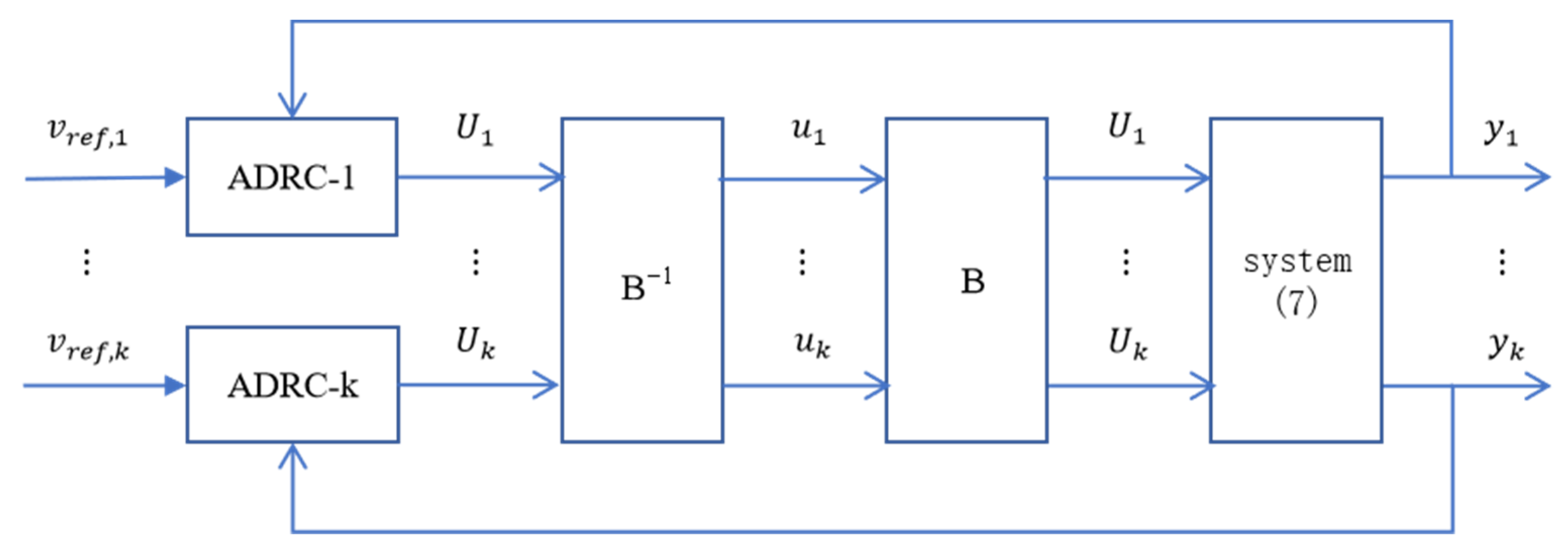
• The mismatched uncertainty model for NMVs was established considering the large range of parameter uncertainty and external disturbance. A cascade ADRC method was developed for a class of multi-input multioutput high-order coupled system.
• According to the model characteristics of NMV, both linear active disturbance rejection control (LADRC) and nonlinear active disturbance rejection control (NLADRC) were designed for velocity and altitude subsystems of NMVs. Furthermore, the stabilization of the cascade closed-loop and switching control systems were analyzed.
• A novel switching control strategy based on the interval type-2 fuzzy logic system was developed. Furthermore, both fuzzy rules and the corresponding results of the velocity and altitude subsystems were examined, and the defuzzification algorithm of each step was established.
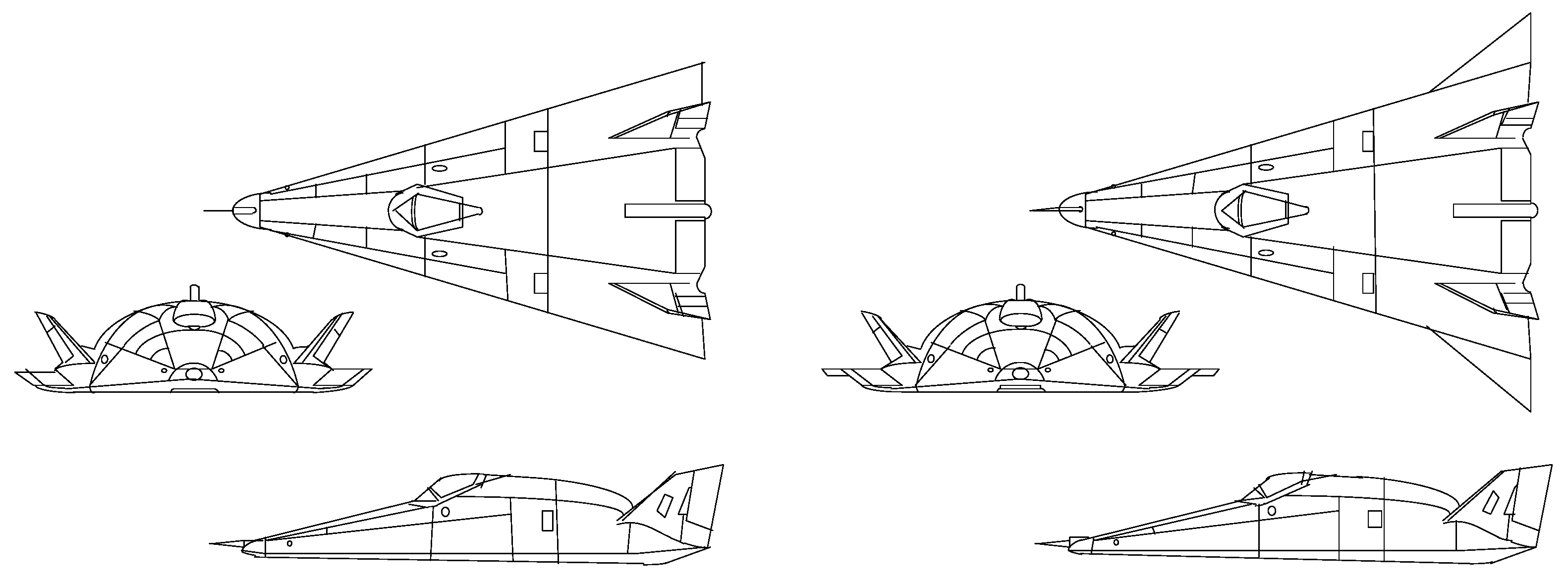
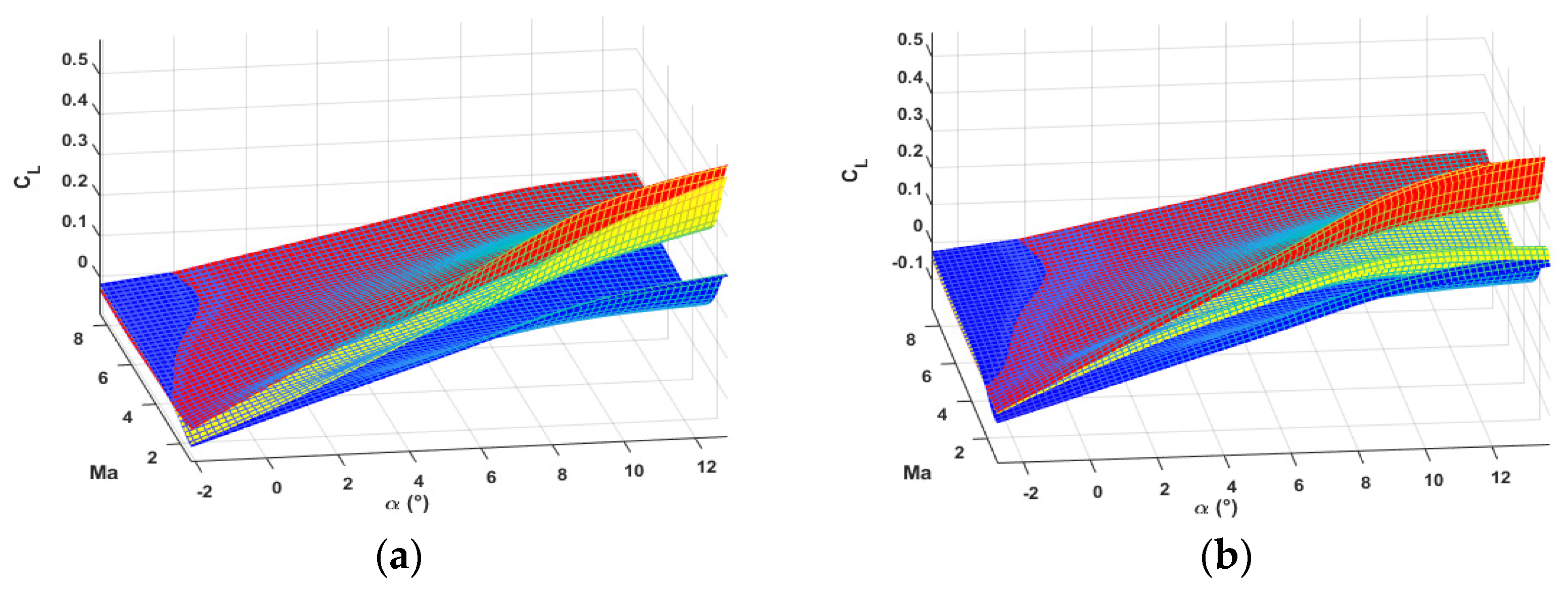
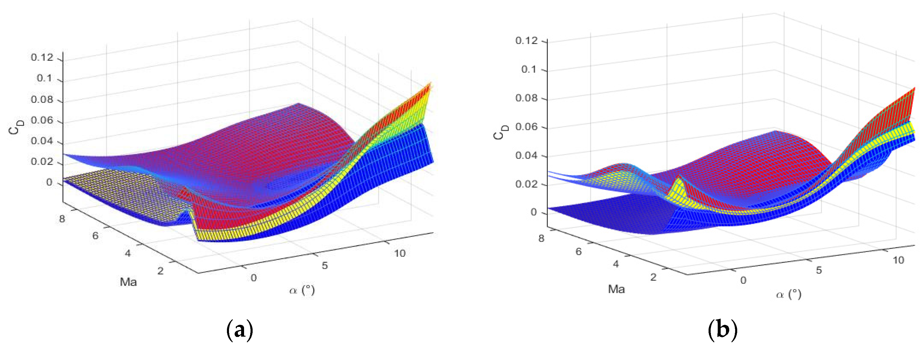
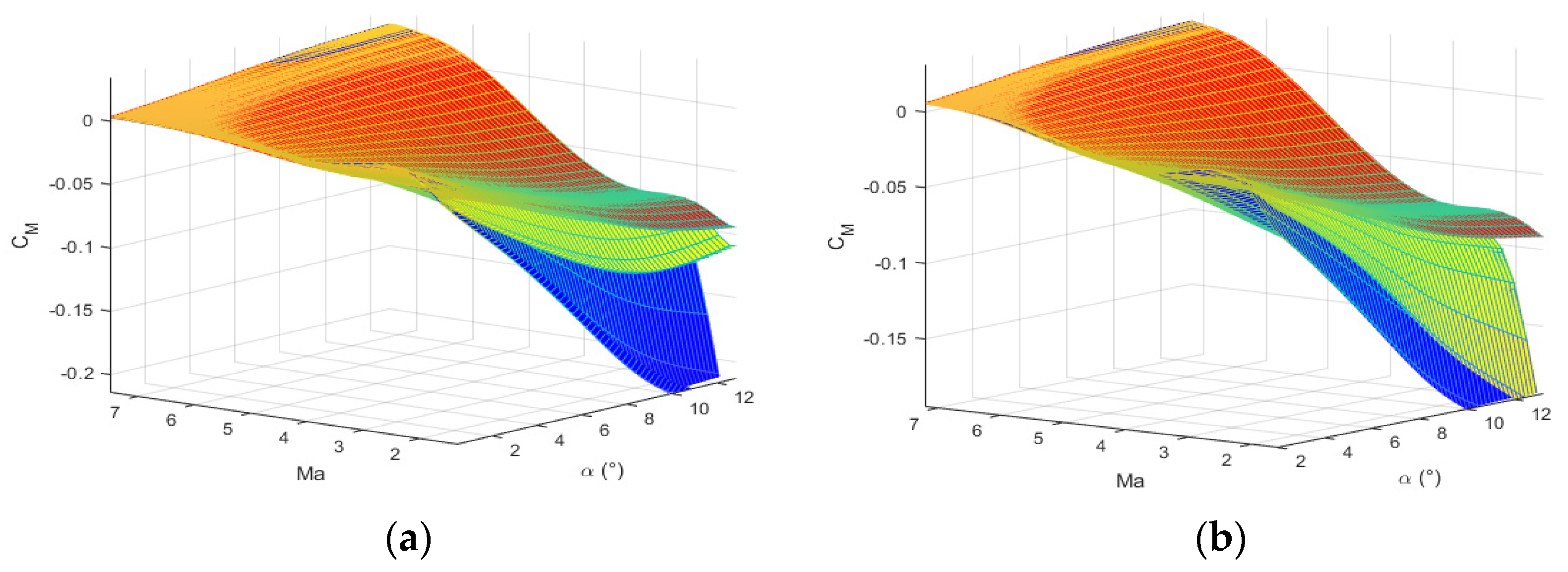
• The change rules of aerodynamic parameters with Mach number and angle of attack under the condition of winglet stretch out and draw back were analyzed. The efficiency and robustness of the proposed control method were demonstrated by numerical simulations.

The remainder of this paper is organized as follows. In Section 2, the mismatched uncertainty model for NMVs is established considering the large range of parameter uncertainty and external disturbance. Section 3 presents the linear and nonlinear cascade ADRC design methods for NMVs and proposes a novel switching control strategy based on the interval type-2 fuzzy logic system. The NMV case simulations and discussions are provided in Section 4, followed by the conclusion in Section 5.

2. NMV Model Description

This paper is concerned with the problems of robust switching control for NMVs. Illustrations of typical NMV modes based on X-24B configuration [28] are shown in Figure 1. The data come from an experimental aircraft model, and the winglets were used to adjust the lift-drag ratio, mean aerodynamic chord, and reference area.

According to [28,29], based on reasonable assumption, the nonlinear equations of the longitudinal motion are formulated as

$$\left\{\begin{array}{l}\dot{V}=\frac{T\cos \alpha -D}{m}-g\sin \gamma \\ \dot{h}=V\sin \gamma \\ \dot{\gamma }=\frac{L+T\sin \alpha }{mV}-\frac{g\cos \gamma }{V}\\ \dot{\alpha }=q-\dot{\gamma }\\ \dot{q}=M_{yy}/I_{yy}\\ \ddot{\eta }=-2\zeta {\omega }_n\dot{\eta }-{\omega }_n^2\eta +{\omega }_n^2{\eta }_c\end{array}\right.$$

(1)

where $V,h,\gamma ,\alpha$, and $q$ are flight velocity, flight altitude, flight path angle, angle of attack, and pitch angle rate, respectively. ${\omega }_n,\zeta$, and ${\eta }_c$ represent natural frequency, damp ratio, and throttle setting, respectively. The lift, drag, thrust, and pitching moment are given as follows:

$$\left\{\begin{array}{l}L=0.5\rho V^{2}s{C}_L\\ D=0.5\rho V^{2}s{C}_D\\ T=0.5\rho V^{2}s{C}_T\\ M_{yy}=0.5\rho V^{2}s\overline{c}(C_M^{\alpha }+C_M^q+C_M^{{\delta }_e})\end{array}\right.$$

(2)

where $\rho ,s$, and $\overline{c}$ stand for the air density, reference area, and mean aerodynamic chord, respectively. The coefficients $C_L,C_D,C_T,C_M^{\alpha },C_M^q$, and $C_M^{{\delta }_e}$ are modeled by data fitting, and the approximations are given as follows:

$$\left\{\begin{array}{l}{C}_L=C_L^{\alpha }\alpha +C_L^0\\ C_D=C_D^{{\alpha }^2}{\alpha }^2+C_D^{\alpha }\alpha +C_D^0\\ C_T=C_T^{\eta }\eta +C_T^0\\ C_M^{\alpha }=C_M^{\alpha ,{\alpha }^2}{\alpha }^2+C_M^{\alpha ,\alpha }\alpha +C_M^{\alpha ,0}\\ C_M^q=C_M^{q,{\alpha }^2}{\alpha }^2+C_M^{q,\alpha }\alpha +C_M^{q,0}\\ C_M^{{\delta }_e}=c_e({\delta }_e-\alpha )\end{array}\right.$$

(3)

According to the nonlinear system theory, the state vector $x=\left[V,\gamma ,\alpha ,\eta ,h\right]$ can be defined. If there are no parameter uncertainties, the input–output feedback linearization method can be adopted for model (1), and we obtain

$$\left[\begin{array}{c}\stackrel{⃛}{V}\\ h^{(4)}\end{array}\right]=\left[\begin{array}{c}{F}_V\\ F_h\end{array}\right]+\left[\begin{array}{cc}{b}_{11}& b_{12}\\ b_{21}& b_{22}\end{array}\right]\left[\begin{array}{c}{\eta }_c\\ {\delta }_e\end{array}\right]$$

(4)

where the control input $u={\left[{\eta }_c,{\delta }_e\right]}^{\mathrm{T}}$, $F_V,F_h,b_{11},b_{12},b_{21},b_{22}$ can be obtained as follows [28]:

$$\left\{\begin{array}{l}{F}_v=\frac{{\omega }_1{\ddot{X}}_0+{\dot{x}}^{\mathrm{T}}{\Omega }_2\dot{x}}{m}\\ F_h=3\ddot{V}\dot{\gamma }\cos \gamma -3\dot{V}{\gamma }^2\sin \gamma +3\dot{V}\ddot{\gamma }\cos \gamma -V{\dot{\gamma }}^3\cos \gamma -3V\dot{\gamma }\ddot{\gamma }\sin \gamma +f(V,\gamma )\\ f(V,\gamma )=\frac{\left({\omega }_1{\ddot{X}}_0+{\dot{x}}^{\mathrm{T}}{\Omega }_2\dot{x}\right)\sin \gamma }{m}+V\cos \gamma \left({\dot{x}}^{\mathrm{T}}{\Pi }_2\dot{x}+{\pi }_1{\ddot{X}}_0\right)\\ b_{11}=\frac{\rho V^{2}s{c}_{\beta }{\omega }_n^2}{2m}\cos \alpha \\ b_{12}=-\frac{\rho V^{2}s\overline{c}{c}_e}{2m{I}_y}(T\sin \alpha +D_{\alpha })\\ b_{21}=\frac{\rho V^{2}s{c}_{\beta }{\omega }_n^2}{2m}\sin (\alpha +\gamma )\\ b_{22}=\frac{\rho V^{2}s\overline{c}{c}_e}{2m{I}_y}\left[T\cos (\alpha +\gamma )+L_{\alpha }\cos \gamma -D_{\alpha }\sin \gamma \right]\end{array}\right.$$

(5)

where ${\omega }_1=\partial f_1(x)/\partial x$, $f_1(x)=T\cos \alpha -D-mg\sin \gamma$, ${\Omega }_2=\partial {\omega }_1/\partial x$, ${\pi }_1=\partial f_2(x)/\partial x$, $f_2(x)=(L+T\sin \alpha )/mV-g\cos \gamma /V$, ${\Pi }_2=\partial {\pi }_1/\partial x$.

If all the parameters of NMVs are considered to be uncertain, they are expressed as $i=i_0+\Delta i$, $i=m$, $s$, $\overline{c}$, $c_e$, $I_{yy}$, $C_L^{\alpha }$, $C_L^0$, $C_D^{{\alpha }^2}$, $C_D^{\alpha }$, $C_D^0$, $C_T^{\eta }$, $C_T^0$, $C_M^{\alpha ,{\alpha }^2}$, $C_M^{\alpha ,\alpha }$, $C_M^{\alpha ,0}$, $C_M^{q,{\alpha }^2}$, $C_M^{q,\alpha }$, $C_M^{q,0}$, where $i$ represents the real value, $i_0$ denotes the nominal value, $\Delta i=i_0\cdot \Lambda \%\cdot \sin (\omega t)$, and $\Lambda \%$ represents the parameters’ uncertain boundary. Furthermore, if mismatched external disturbance is considered, then Equation (4) can rewritten as follows:

$$\left\{\begin{array}{l}{\dot{V}}_1=V_2+{\phi }_{V_1}+d_{V_1}\\ {\dot{V}}_2=V_3+{\phi }_{V_2}+d_{V_2}\\ {\dot{V}}_3=F_V+b_{11}{\eta }_c+b_{12}{\delta }_e+{\phi }_{V_3}+d_{V_3}\\ {\dot{h}}_1=h_2+{\phi }_{h_1}+d_{h_1}\\ {\dot{h}}_2=h_3+{\phi }_{h_2}+d_{h_2}\\ {\dot{h}}_3=h_4+{\phi }_{h_3}+d_{h_3}\\ {\dot{h}}_4=F_h+b_{21}{\eta }_c+b_{22}{\delta }_e+{\phi }_{h_4}+d_{h_4}\end{array}\right.$$

(6)

where $V_1,V_2,V_3$ and $h_1,h_2,h_3,h_4$ are states of the velocity and altitude subsystems, respectively; ${\phi }_{V_1},{\phi }_{V_2},{\phi }_{V_3}$ and ${\phi }_{h_1},{\phi }_{h_2},{\phi }_{h_3},{\phi }_{h_4}$ represent the parameters’ uncertain terms for the velocity and altitude subsystems, respectively; and $d_{V_1},d_{V_2},d_{V_3}$ and $d_{h_1},d_{h_2},d_{h_3},d_{h_4}$ represent the mismatching external disturbance of the velocity and altitude subsystems, respectively.

3. Controller Design

3.1. ADRC for Multivariate Coupled Systems

Without loss of generality, the multivariable coupling system can be considered as follows:

$$\left\{\begin{array}{l}{x}_{s_1}^{(n_1)}=f_{s_1}+b_{11}{u}_1+b_{12}{u}_2+\cdots +b_{1k}{u}_k\\ y_{s_1}=x_{s_1,1}\\ x_{s_2}^{(n_2)}=f_{s_2}+b_{21}{u}_1+b_{22}{u}_2+\cdots +b_{2k}{u}_k\\ y_{s_2}=x_{s_2,1}\\ ⋮\\ x_{s_k}^{(n_k)}=f_{s_k}+b_{k1}{u}_1+b_{k2}{u}_2+\cdots +b_{kk}{u}_k\\ y_{s_k}=x_{s_k,1}\end{array}\right.$$

(7)

where $x_{s_i}(i=1,2,\cdots ,k)$ represents the system states, $b_{ij}(i,j=1,2,\cdots ,k)$ represents the coefficients of the control input, and $f_{s_i}(i=1,2,\cdots ,k)$ represents the whole disturbance of each channel, which can be estimated and compensated by ADRC. Defining $x={\left[x_{s_1},x_{s_2},\cdots ,x_{s_k}\right]}^{\mathrm{T}}$, $y={\left[y_{s_1},y_{s_2},\cdots ,y_{s_k}\right]}^{\mathrm{T}}$, $f={\left[f_{s_1},f_{s_2},\cdots ,f_{s_k}\right]}^{\mathrm{T}}$, $u={\left[u_1,u_2,\cdots ,u_k\right]}^{\mathrm{T}}$, and $n_1=n_2=\cdots =n_k=n$, system (6) can be described in brief as

$$\left\{\begin{array}{l}{x}^{(n)}=f+Bu=f+U\\ y=x\end{array}\right.,B=\left[\begin{array}{ccc}{b}_{11}& \cdots & b_{1k}\\ ⋮& ⋮& ⋮\\ b_{k1}& \cdots & b_{kk}\end{array}\right]$$

(8)

Furthermore, for any $ith$ channel of system (8), it has

$$\left\{\begin{array}{l}{x}_i^{(n)}=f_i+U_i\\ y_i=x_i\end{array}\right.$$

(9)

Equation (9) shows that a single input single output relationship is formed between the virtual control quantity $U_i$ and the output quantity $y_i$, that is, complete decoupling between the output quantity $y_i$ and the virtual control quantity $U_i$ is realized. Therefore, if the controlled quantity $y_i$ can be measured, the target $y_{id}$ can be tracked by designing an ADRC. The block diagram of the ADRC for a multivariable coupling system is shown in Figure 2.

It can be seen from Figure 1 that there are k ADRC systems embedded in parallel between the control quantity $U_i$ and the output quantity $y_i$, and each ADRC system is composed of n first-order ADRC controllers in series; thus, the cascade decoupled control for high-order multivariate coupled systems is realized.

3.2. Linear/Nonlinear Extended State Observer Design

Assuming $x_1=x$, $x_2=\dot{x}$, $\cdots$, $x_n=x^{(n-1)}$, and $x_{n+1}=f(\cdot )$ represents the extended state variable of the system, then the general form of the continuous extended state observer (ESO) is correspondingly designed as

$$\left\{\begin{array}{l}e=z_1-y\\ {\dot{z}}_1=z_2-{\beta }_1\cdot g_1(e)\\ {\dot{z}}_2=z_3-{\beta }_2\cdot g_2(e)\\ ⋮\\ {\dot{z}}_n=z_{n+1}-{\beta }_n\cdot g_n(e)+b\cdot u\\ {\dot{z}}_{n+1}=-{\beta }_{n+1}\cdot g_{n+1}(e)\end{array}\right.$$

(10)

where $z_i(i=1,2,\cdots ,n+1)$ represents the estimates of the state variable $x_i(i=1,2,\cdots ,n)$, and total disturbance $x_{n+1}=f(\cdot )$, $g_i(e)(i=1,2,\cdots ,n+1)$ represents the function of estimation error $e$. Under specific conditions, ESO can accurately estimate the various states of the object and the total disturbance of the system. Then, we have

$$\left\{\begin{array}{l}{z}_1\to x_1\\ z_2\to x_2\\ ⋮\\ z_n\to x_n\\ z_{n+1}\to f(\cdot )\end{array}\right.$$

(11)

When $g_i(e)(i=1,2,\cdots ,n+1)$ is a select nonlinear function, ESO (10) is a nonlinear extended state observer (NESO). The specific nonlinear function can be express as

$$g_i(e)=\mathrm{fal}(e,{\alpha }_i,\delta )=\left\{\begin{array}{c}{\left|e\right|}^{{\alpha }_i}\mathrm{sign}(e),\left|e\right|>\delta \\ \frac{e}{{\delta }^{1-{\alpha }_i}},\left|e\right|\le \delta \end{array}\right.$$

(12)

where $0<{\alpha }_i<1$, $\delta >0$; it is worthy to point out that when ${\alpha }_i=1$, then $g_i(e)=e$, and the ESO (10) is a linear extended state observer (LESO), which can be rewritten as

$$\left\{\begin{array}{l}e=z_1-y\\ {\dot{z}}_1=z_2-{\beta }_1^{\prime }\cdot e\\ {\dot{z}}_2=z_3-{\beta }_2^{\prime }\cdot e\\ ⋮\\ {\dot{z}}_n=z_{n+1}-{\beta }_n^{\prime }\cdot e+b\cdot u\\ {\dot{z}}_{n+1}=-{\beta }_{n+1}^{\prime }\cdot e\end{array}\right.$$

(13)

Theoretical analysis and simulation research indicate that LESO parameter tuning is convenient, theoretical analysis is simple, and the disturbance tracking performance hardly changes with the disturbance amplitude. The parameter tuning of NESO is complex and theoretical analysis is difficult, but it has advantages such as high parameter efficiency, high tracking accuracy, and fast response speed. In order to fully utilize the advantages of LESO and NESO, this paper proposes a LESO/NESO switching control strategy based on the interval type-2 fuzzy logic system.

3.3. Cascade ADRC Design

According to the NMV model (6), the velocity channel can be described as

$$\left\{\begin{array}{l}{\dot{x}}_{V_1}=x_{V_2}+g_{V_1}\\ {\dot{x}}_{V_2}=x_{V_3}+g_{V_2}\\ {\dot{x}}_{V_3}=F_V+g_{V_3}+u_V\\ y=x_{V_1}\end{array}\right.$$

(14)

where $x_{V_1},x_{V_2},x_{V_3}$ are states of the velocity subsystem; $g_{V_i}={\phi }_{V_i}+d_{V_i}(i=1,2,3)$ represents the mismatched uncertain terms, including the parameters uncertain terms ${\phi }_{V_i}$; and the mismatching external disturbance terms $d_{V_i}$, $u_V=b_{11}{\eta }_c+b_{12}{\delta }_e$ represent the control input of the velocity channel. System (14) is a third-order system with uncertain parameters and mismatching external disturbance. The control objective is to enable variable $x_{V_1}$ to quickly track reference signal $V_{ref}$. The design idea of cascade ADRC is to convert system (14) into three first-order systems and design three ADRCs, respectively. The specific steps can be described as follows.

Step 1: Regard $x_{V_2}$ as a virtual control quantity. Then, the auto disturbance rejection algorithm for the $x_{V_1}$ tracking reference signal $V_{ref}$ can be described as

$$\left\{\begin{array}{l}{e}_V=V_1-V_{ref}\\ {\dot{V}}_1=-r_{V_0}\mathrm{fal}(e_V,{\alpha }_{V_0},{\delta }_{V_0})\\ e_{V_1,1}=z_{V_1,1}-x_{V_1}\\ {\dot{z}}_{V_1,1}=z_{V_1,2}-{\beta }_{V_1,1}{e}_{V_1,1}+u_{V_1}\\ {\dot{z}}_{V_1,2}=-{\beta }_{V_1,2}\mathrm{fal}(e_{V_1,1},{\alpha }_{V_1},{\delta }_{V_1})\\ e_{V_1,2}=V_1-z_{V_1,1}\\ u_{V_1}={\beta }_{V_1,u}\mathrm{fal}(e_{V_1,2},{\alpha }_{V_1,u},{\delta }_{V_1,u})-z_{V_1,2}\end{array}\right.$$

(15)

Step 2: Regard $x_{V_3}$ as a virtual control quantity. Then, the auto disturbance rejection algorithm for the $x_{V_2}$ tracking reference signal $u_{V_1}$ can be described as

$$\left\{\begin{array}{l}{e}_{V_2,1}=z_{V_2,1}-x_{V_2}\\ {\dot{z}}_{V_2,1}=z_{V_2,2}-{\beta }_{V_2,1}{e}_{V_2,1}+u_{V_2}\\ {\dot{z}}_{V_2,2}=-{\beta }_{V_2,2}\mathrm{fal}(e_{V_2,1},{\alpha }_{V_2},{\delta }_{V_2})\\ e_{V_2,2}=u_{V_1}-z_{V_2,1}\\ u_{V_2}={\beta }_{V_2,u}\mathrm{fal}(e_{V_2,2},{\alpha }_{V_2,u},{\delta }_{V_2,u})-z_{V_2,2}\end{array}\right.$$

(16)

Step 3: Let actual control law $u_V$ control the state variable $x_{V_3}$. Then, the auto disturbance rejection algorithm for $x_{V_3}$ tracking reference signal $u_{V_2}$ can be described as

$$\left\{\begin{array}{l}{e}_{V_3,1}=z_{V_3,1}-x_{V_3}\\ {\dot{z}}_{V_3,1}=z_{V_3,2}-{\beta }_{V_3,1}{e}_{V_3,1}+u_V\\ {\dot{z}}_{V_3,2}=-{\beta }_{V_3,2}\mathrm{fal}(e_{V_3,1},{\alpha }_{V_3},{\delta }_{V_3})\\ e_{V_3,2}=u_{V_2}-z_{V_3,1}\\ u_V={\beta }_{V_3,u}\mathrm{fal}(e_{V_3,2},{\alpha }_{V_3,u},{\delta }_{V_3,u})-z_{V_3,2}\end{array}\right.$$

(17)

Equations (15)–(17) express cascade NLADRC for system (14), and the $\mathrm{fal}(\cdot )$ is set as Equation (12). When $\mathrm{fal}(\cdot )$ is replaced by linear function of errors, Equations (15)–(17) express cascade LADRC for system (14). The altitude channel can be designed in the same way, which will not be repeated here. It is worth noting that in order to enable the ADRC to achieve better results, the transition process is designed in the first stage of ADRC of the velocity and altitude channels. The purpose is to achieve the output of the first stage as slowly as possible. However, when designing the following ADRC, the purpose is to let the state variables of the next stage track the virtual control quantity of the previous stage as quickly as possible, so the transition process is canceled in the ADRC of the next several stages.

3.4. Cascade ADRC Convergence Analysis

Considering the velocity channel subsystem (14) and the cascade NLADRC (15)–(17), the convergence of the system was analyzed.

For convenience of analysis, the transformations were defined as follows:

$$\mathrm{fal}(e_{V_i,1},{\alpha }_{V_1},{\delta }_{V_1})=\frac{\mathrm{fal}(e_{V_i,1},{\alpha }_{V_1},{\delta }_{V_1})}{e_{V_i,1}}{e}_{V_i,1}={\lambda }_{V_i,1}(e_{V_i,1})e_{V_i,1},(i=1,2,3)$$

(18)

Then, according to Equations (15)–(17), the following is obtained:

$$\left\{\begin{array}{l}{\ddot{z}}_{V_1,1}+{\beta }_{V_1,1}{\dot{z}}_{V_1,1}+{\beta }_{V_1,2}{\lambda }_{V_1,1}(e_{V_1,1})z_{V_1,1}={\beta }_{V_1,1}{\dot{x}}_{V_1}+{\beta }_{V_1,2}{\lambda }_{V_1,1}(e_{V_1,1})x_{V_1}+{\dot{u}}_{V_1}\\ {\ddot{z}}_{V_2,1}+{\beta }_{V_2,1}{\dot{z}}_{V_2,1}+{\beta }_{V_2,2}{\lambda }_{V_2,1}(e_{V_2,1})z_{V_2,1}={\beta }_{V_2,1}{\dot{x}}_{V_2}+{\beta }_{V_2,2}{\lambda }_{V_2,1}(e_{V_2,1})x_{V_2}+{\dot{u}}_{V_2}\\ {\ddot{z}}_{V_3,1}+{\beta }_{V_3,1}{\dot{z}}_{V_3,1}+{\beta }_{V_3,2}{\lambda }_{V_3,1}(e_{V_3,1})z_{V_3,1}={\beta }_{V_3,1}{\dot{x}}_{V_3}+{\beta }_{V_3,2}{\lambda }_{V_3,1}(e_{V_3,1})x_{V_3}+{\dot{u}}_V\end{array}\right.$$

(19)

where $e_{V_1,1}=z_{V_1,1}-x_{V_1}$, $e_{V_1,2}=z_{V_1,2}-x_{V_2}$, and $e_{V_1,3}=z_{V_1,3}-x_{V_3}$ represent the state estimation errors of each stage. According to the design idea of cascade ADRC, the following applies:

$$\left\{\begin{array}{l}{x}_{V_2}\to u_{V_1}\\ x_{V_3}\to u_{V_2}\end{array}\right.$$

(20)

Substituting Equation (20) into (14), we can obtain

$$\left\{\begin{array}{l}{\dot{u}}_{V_1}={\ddot{x}}_{V_1}-{\dot{g}}_{V_1}\\ {\dot{u}}_{V_2}={\ddot{x}}_{V_2}-{\dot{g}}_{V_2}\\ {\dot{u}}_V={\ddot{x}}_{V_3}-{\dot{L}}_x\end{array}\right.$$

(21)

where $L_x=F_V+g_{V_3}$. Then, substituting Equation (21) into (19), we have

$$\left\{\begin{array}{l}{\ddot{z}}_{V_1,1}+{\beta }_{V_1,1}{\dot{z}}_{V_1,1}+{\beta }_{V_1,2}{\lambda }_{V_1,1}(e_{V_1,1})z_{V_1,1}={\beta }_{V_1,1}{\dot{x}}_{V_1}+{\beta }_{V_1,2}{\lambda }_{V_1,1}(e_{V_1,1})x_{V_1}+{\ddot{x}}_{V_1}-{\dot{g}}_{V_1}\\ {\ddot{z}}_{V_2,1}+{\beta }_{V_2,1}{\dot{z}}_{V_2,1}+{\beta }_{V_2,2}{\lambda }_{V_2,1}(e_{V_2,1})z_{V_2,1}={\beta }_{V_2,1}{\dot{x}}_{V_2}+{\beta }_{V_2,2}{\lambda }_{V_2,1}(e_{V_2,1})x_{V_2}+{\ddot{x}}_{V_2}-{\dot{g}}_{V_2}\\ {\ddot{z}}_{V_3,1}+{\beta }_{V_3,1}{\dot{z}}_{V_3,1}+{\beta }_{V_3,2}{\lambda }_{V_3,1}(e_{V_3,1})z_{V_3,1}={\beta }_{V_3,1}{\dot{x}}_{V_3}+{\beta }_{V_3,2}{\lambda }_{V_3,1}(e_{V_3,1})x_{V_3}+{\dot{u}}_V-{\dot{L}}_x\end{array}\right.$$

(22)

furthermore have

$$\left\{\begin{array}{l}{\ddot{e}}_{V_1,1}+{\beta }_{V_1,1}{\dot{e}}_{V_1,1}={\dot{z}}_{V_1,2}-{\dot{g}}_{V_1}\\ {\ddot{e}}_{V_2,1}+{\beta }_{V_2,1}{\dot{e}}_{V_2,1}={\dot{z}}_{V_2,2}-{\dot{g}}_{V_2}\\ {\ddot{e}}_{V_3,1}+{\beta }_{V_3,1}{\dot{e}}_{V_3,1}={\dot{z}}_{V_3,2}-{\dot{L}}_x\end{array}\right.$$

(23)

If the mismatched uncertain terms $g_{V_i}={\phi }_{V_i}+d_{V_i}(i=1,2,3)$ in system (14) and its first-order differential are bounded, that is $\left|g_{V_i}\right|\le \delta$, $\left|{\dot{g}}_{V_i}\right|\le \overline{\delta }$, where $\delta ,\overline{\delta }$ are known normal numbers, the total disturbance estimation errors $e_{V_1,2}=z_{V_1,2}-g_{V_1}$, $e_{V_2,2}=z_{V_2,2}-g_{V_2}$, and $e_{V_3,2}=z_{V_3,2}-L_x$ for each stage in Equation (23) can be described as

$$\left\{\begin{array}{l}{\dot{e}}_{V_1,1}+{\beta }_{V_1,1}{e}_{V_1,1}=e_{V_1,2}\\ {\dot{e}}_{V_2,1}+{\beta }_{V_2,1}{e}_{V_2,1}=e_{V_2,2}\\ {\dot{e}}_{V_3,1}+{\beta }_{V_3,1}{e}_{V_3,1}=e_{V_3,2}\end{array}\right.$$

(24)

As can be seen from Equation (24), when the appropriate controller parameters are selected, the state estimation errors in each stage converge exponentially. According to the transmission characteristics of the cascade controller, the inner loop system is generally required to be stable before the outer loop system, that is, the movement of the inner loop changes faster than that of the outer loop, that is, the time scale of the inner loop system is smaller than that of the outer loop system. Therefore, in the actual numerical simulation, the sampling step of the inner loop should be smaller than that of the outer loop. According to experience, the sampling step size of the outer loop is generally selected as an integral multiple of the sampling step size of the inner loop.

3.5. Stable Analysis of LADRC/NLADRC Switching

The switching between LADRC and NADRC is essentially the switching between LESO and NLESO. Therefore, a simple switching stability analysis method between LESO and NLESO is given as follows.

Consider the following system

$$\left\{\begin{array}{l}e=z_1-y\\ {\dot{z}}_1=z_2-{\beta }_{1}e\\ {\dot{z}}_2=z_3-{\beta }_2\mathrm{fal}(e,{\alpha }_2,{\delta }_2)+bu\\ {\dot{z}}_3=-{\beta }_3\mathrm{fal}(e,{\alpha }_3,{\delta }_3)\end{array}\right.$$

(25)

Define

$$\left\{\begin{array}{l}\mathrm{fal}(e,{\alpha }_2,{\delta }_2)=\frac{\mathrm{fal}(e,{\alpha }_2,{\delta }_2)}{e}e={\lambda }_2(e)e\\ \mathrm{fal}(e,{\alpha }_3,{\delta }_3)=\frac{\mathrm{fal}(e,{\alpha }_3,{\delta }_3)}{e}e={\lambda }_3(e)e\end{array}\right.$$

(26)

Then, the Equation (25) can be rewrite as

$$\left\{\begin{array}{l}e=z_1-y\\ {\dot{z}}_1=z_2-{\beta }_{1}e\\ {\dot{z}}_2=z_3-{\beta }_2{\lambda }_2(e)e+bu\\ {\dot{z}}_3=-{\beta }_3{\lambda }_3(e)e\end{array}\right.$$

(27)

Both ${\beta }_2{\lambda }_2(e)$ and ${\beta }_3{\lambda }_3(e)$ in Equation (23) can be regarded as the gain coefficient of the error $e=z_1-y$. Because the error gain coefficients ${\beta }_2{\lambda }_2(e)$ and ${\beta }_3{\lambda }_3(e)$ are the function of the error, it can be understood that the variation range of the gain coefficient is within a perturbation range related to the error. Then, when an equivalent perturbation range independent of error is selected to replace the gain coefficient, the system (27) can be regarded as a linear extended state observer with variable gain. Its transfer function model can be described as

$$\left\{\begin{array}{l}{z}_1=\frac{({\beta }_1{s}^2+{\beta }_2{\lambda }_{2}s+{\beta }_3{\lambda }_3)\cdot y+bu\cdot s}{s^3+{\beta }_1{s}^2+{\beta }_2{\lambda }_{2}s+{\beta }_3{\lambda }_3}\\ z_2=\frac{({\beta }_2{\lambda }_{2}s+{\beta }_3{\lambda }_3)\cdot y\cdot s+(s+{\beta }_1)\cdot bu\cdot s}{s^3+{\beta }_1{s}^2+{\beta }_2{\lambda }_{2}s+{\beta }_3{\lambda }_3}\\ z_3=\frac{{\beta }_3{\lambda }_2\cdot y\cdot s^2-{\beta }_3{\lambda }_3\cdot bu-{\beta }_3{\lambda }_3\cdot f(s)}{s^3+{\beta }_1{s}^2+{\beta }_2{\lambda }_{2}s+{\beta }_3{\lambda }_3}\end{array}\right.$$

(28)

As can be seen from Equation (28), the sufficient and necessary condition for the stability of the system (25) is ${\beta }_1{\beta }_2{\lambda }_2>{\beta }_3{\lambda }_3$. When $\mathrm{fal}(e,{\alpha }_2,{\delta }_2)=\mathrm{fal}(e,{\alpha }_3,{\delta }_3)$, we can obtain ${\lambda }_2={\lambda }_3$ and then ${\beta }_1{\beta }_2>{\beta }_3$.

For stable NLESO, the poles of the transfer function model (28) are located in a region of the left half plane. When switching between LESO and NLESO, in order to ensure the stability of switching, the poles of LESO also need to be in the same area of the left half plane [31,32]. Therefore, the sufficient and necessary condition for the switching stability between LESO and NLESO is that the parameters of LESO should meet.

$$\left\{\begin{array}{l}{\beta }_2{({\lambda }_2(e))}_{\min }<{\beta }_2^{*}<{\beta }_2{({\lambda }_2(e))}_{\max }\\ {\beta }_3{({\lambda }_3(e))}_{\min }<{\beta }_3^{*}<{\beta }_3{({\lambda }_3(e))}_{\max }\end{array}\right.$$

(29)

According to the above analysis, reasonable selection parameters for ESO can ensure the stability of switching between LESO and NLESO.

3.6. Switch Control Strategy Based on the Interval Type-2 Fuzzy Logic System

A large number of simulation studies show that LESO has the characteristics of convenient parameter tuning, simple theoretical analysis, and strong anti-interference ability. NLESO has the advantages of high parameter efficiency, fast response speed, and high control accuracy, but it lacks the ability to estimate large disturbances and oscillations can be generated easily. The type-2 fuzzy logic system can increase the degree of freedom for the membership function [23]. It is easier to achieve smooth switching between LADRC and nonlinear NLADRC.

According to the characteristics of NMVs, when NMVs ascend, the wingspan and wing area are increased by extending the winglet so as to obtain higher aspect ratio, lift drag ratio, and increase the lift. When NMVs cruise, the force area is reduced by retracting the winglet, thus reducing drag and improving the flight efficiency. However, the retraction change of the winglet will directly lead to the change of the wing area and the average aerodynamic chord length, thus changing the aerodynamic parameters, aerodynamic forces, and aerodynamic moments of the NMV. Therefore, considering mismatched uncertainties, LADRC and NLADRC are used for ascent modality and cruise modality, respectively, in order for the NMV to achieve stable flight under each modality, and the switching control strategy based on the interval type-2 fuzzy logic system is adopted to realize stable flight control during multimode switching.

In the switching process, the system state tracking error $\left|e_V\right|=\left|V_1-V_{ref}\right|$ $\left|e_h\right|=\left|h_1-h_{ref}\right|$ and disturbance observation error $\left|e_{gi}\right|(i=V,h)$ are set as the inputs of the fuzzy controller. The weights of LADRC and NLADRC are set as outputs of the fuzzy controller. Then, fuzzy rules can be described as follows:

Velocity channel subsystem

$R_V^1$: If $\left|e_V\right|$ is S and $\left|e_{g_V}\right|$ is S, Then $u_{cV,L}$ is $Y_L^1$ and $u_{cV,N}$ is $Y_N^1$

$R_V^2$: If $\left|e_V\right|$ is S and $\left|e_{g_V}\right|$ is M, Then $u_{cV,L}$ is $Y_L^2$ and $u_{cV,N}$ is $Y_N^2$

$R_V^3$: If $\left|e_V\right|$ is S and $\left|e_{g_V}\right|$ is B, Then $u_{cV,L}$ is $Y_L^3$ and $u_{cV,N}$ is $Y_N^3$

$R_V^4$: If $\left|e_V\right|$ is M and $\left|e_{g_V}\right|$ is S, Then $u_{cV,L}$ is $Y_L^4$ and $u_{cV,N}$ is $Y_N^4$

$R_V^5$: If $\left|e_V\right|$ is M and $\left|e_{g_V}\right|$ is M, Then $u_{cV,L}$ is $Y_L^5$ and $u_{cV,N}$ is $Y_N^5$

$R_V^6$: If $\left|e_V\right|$ is M and $\left|e_{g_V}\right|$ is B, Then $u_{cV,L}$ is $Y_L^6$ and $u_{cV,N}$ is $Y_N^6$

$R_V^7$: If $\left|e_V\right|$ is B and $\left|e_{g_V}\right|$ is S, Then $u_{cV,L}$ is $Y_L^7$ and $u_{cV,N}$ is $Y_N^7$

$R_V^8$: If $\left|e_V\right|$ is B and $\left|e_{g_V}\right|$ is M, Then $u_{cV,L}$ is $Y_L^8$ and $u_{cV,N}$ is $Y_N^8$

$R_V^9$: If $\left|e_V\right|$ is B and $\left|e_{g_V}\right|$ is B, Then $u_{cV,L}$ is $Y_L^9$ and $u_{cV,N}$ is $Y_N^9$

Altitude channel subsystem

$R_h^1$: If $\left|e_h\right|$ is S and $\left|e_{g_h}\right|$ is S, Then $u_{ch,L}$ is $Y_L^1$ and $u_{ch,N}$ is $Y_N^1$

$R_h^2$: If $\left|e_h\right|$ is S and $\left|e_{g_h}\right|$ is M, Then $u_{ch,L}$ is $Y_L^2$ and $u_{ch,N}$ is $Y_N^2$

$R_h^3$: If $\left|e_h\right|$ is S and $\left|e_{g_h}\right|$ is B, Then $u_{ch,L}$ is $Y_L^3$ and $u_{ch,N}$ is $Y_N^3$

$R_h^4$: If $\left|e_h\right|$ is M and $\left|e_{g_h}\right|$ is S, Then $u_{ch,L}$ is $Y_L^4$ and $u_{ch,N}$ is $Y_N^4$

$R_h^5$: If $\left|e_h\right|$ is M and $\left|e_{g_h}\right|$ is M, Then $u_{ch,L}$ is $Y_L^5$ and $u_{ch,N}$ is $Y_N^5$

$R_h^6$: If $\left|e_h\right|$ is M and $\left|e_{g_h}\right|$ is B, Then $u_{ch,L}$ is $Y_L^6$ and $u_{ch,N}$ is $Y_N^6$

$R_h^7$: If $\left|e_h\right|$ is B and $\left|e_{g_h}\right|$ is S, Then $u_{ch,L}$ is $Y_L^7$ and $u_{ch,N}$ is $Y_N^7$

$R_h^8$: If $\left|e_h\right|$ is B and $\left|e_{g_h}\right|$ is M, Then $u_{ch,L}$ is $Y_L^8$ and $u_{ch,N}$ is $Y_N^8$

$R_h^9$: If $\left|e_h\right|$ is B and $\left|e_{g_h}\right|$ is B, Then $u_{ch,L}$ is $Y_L^9$ and $u_{ch,N}$ is $Y_N^9$

In this paper, the primary membership function is the uncertain mean value Gaussian Function (30), and the longitudinal amplitude interval is [0, 1] for the secondary membership function. Figure 3 shows the three-dimensional graph of the Gaussian interval type-2 membership function.

$${\mu }_i^j(x_i)=\exp \left[-\frac{1}{2}{\left(\frac{x_i-{\delta }_i^j}{{\sigma }_i^j}\right)}^2\right], {\delta }_i^j\in \left[{\delta }_{i_1}^j,{\delta }_{i_2}^j\right]$$

(30)

In the switching process, the state tracking error plays a leading role. When the state error is large, the LADRC weight with stronger anti-interference ability is greater than NLADRC. When the state error is small, the NLADRC weight with higher selection efficiency is greater than LADRC. The rule base and corresponding results of LADRC and NLADRC output weights are shown in

Table 1. The rule base and corresponding results for LADRC.

	$\left|{\mathit{e}}_{\mathit{i}}\right|$	S	M	B
$\left|{\mathit{e}}_{\mathit{g}\mathit{i}}\right|$
S		$Y_L^1=\left[{\underset{¯}{y}}_L^1,{\overline{y}}_L^1\right]=\left[0,0.2\right]$	$Y_L^4=\left[{\underset{¯}{y}}_L^4,{\overline{y}}_L^4\right]=\left[0.6,0.4\right]$	$Y_L^7=\left[{\underset{¯}{y}}_L^7,{\overline{y}}_L^7\right]=\left[0.6,0.4\right]$
M		$Y_L^2=\left[{\underset{¯}{y}}_L^2,{\overline{y}}_L^2\right]=\left[0.2,0.4\right]$	$Y_L^5=\left[{\underset{¯}{y}}_L^5,{\overline{y}}_L^5\right]=\left[0.45,0.55\right]$	$Y_L^8=\left[{\underset{¯}{y}}_L^8,{\overline{y}}_L^8\right]=\left[0.8,0.6\right]$
B		$Y_L^3=\left[{\underset{¯}{y}}_L^3,{\overline{y}}_L^3\right]=\left[0.4,0.6\right]$	$Y_L^6=\left[{\underset{¯}{y}}_L^6,{\overline{y}}_L^6\right]=\left[0.6,0.8\right]$	$Y_L^9=\left[{\underset{¯}{y}}_L^9,{\overline{y}}_L^9\right]=\left[1,0.8\right]$

and

Table 2. The rule base and corresponding results for NLADRC.

	$\left|{\mathit{e}}_{\mathit{i}}\right|$	S	M	B
$\left|{\mathit{e}}_{\mathit{g}\mathit{i}}\right|$
S		$Y_N^1=\left[{\underset{¯}{y}}_N^1,{\overline{y}}_N^1\right]=\left[1,0.8\right]$	$Y_N^4=\left[{\underset{¯}{y}}_N^4,{\overline{y}}_N^4\right]=\left[0.4,0.6\right]$	$Y_N^7=\left[{\underset{¯}{y}}_N^7,{\overline{y}}_N^7\right]=\left[0.4,0.6\right]$
M		$Y_N^2=\left[{\underset{¯}{y}}_N^2,{\overline{y}}_N^2\right]=\left[0.8,0.6\right]$	$Y_N^5=\left[{\underset{¯}{y}}_N^5,{\overline{y}}_N^5\right]=\left[0.55,0.45\right]$	$Y_N^8=\left[{\underset{¯}{y}}_N^8,{\overline{y}}_N^8\right]=\left[0.2,0.4\right]$
B		$Y_N^3=\left[{\underset{¯}{y}}_N^3,{\overline{y}}_N^3\right]=\left[0.6,0.4\right]$	$Y_N^6=\left[{\underset{¯}{y}}_N^6,{\overline{y}}_N^6\right]=\left[0.4,0.2\right]$	$Y_N^9=\left[{\underset{¯}{y}}_N^9,{\overline{y}}_N^9\right]=\left[0,0.2\right]$

, respectively, where ${\underset{¯}{y}}_L^i$, ${\underset{¯}{y}}_N^i$, and ${\overline{y}}_L^i$, ${\overline{y}}_N^i$$(i=1,2,\cdots ,9)$ represent the lower bound and upper bound of the weight rule output for LADRC and NLADRC, respectively.

The center of gravity of a type of fuzzy set composed of these single values is found by replacing each regular consequent with a single value located at its center of gravity with a central reducer. The equations can describe as follows:

$$Y_{\cos }(x_i)={\displaystyle \underset{\begin{array}{l}{f}^i\in {\tilde{\mathsf{\Gamma }}}^i\\ y^i\in {\tilde{\Psi }}^i\end{array}}{\cup }\frac{{\displaystyle \sum _{i=1}^n{f}^i{y}^i}}{{\displaystyle \sum _{i=1}^n{f}^i}}}=\left[y_l,y_r\right]$$

(31)

$$y_l=\underset{k\in \left[1,N-1\right]}{\min }\frac{{\displaystyle \sum _{n=1}^k{\underset{¯}{y}}^n{\overline{f}}^n+{\displaystyle \sum _{n=k+1}^N{\underset{¯}{y}}^n{\underset{¯}{f}}^n}}}{{\displaystyle \sum _{n=1}^k{\overline{f}}^n+{\displaystyle \sum _{n=k+1}^N{\underset{¯}{f}}^n}}}$$

(32)

$$y_r=\underset{k\in \left[1,N-1\right]}{\max }\frac{{\displaystyle \sum _{n=1}^k{\overline{y}}^n{\underset{¯}{f}}^n+{\displaystyle \sum _{n=k+1}^N{\overline{y}}^n{\overline{f}}^n}}}{{\displaystyle \sum _{n=1}^k{\underset{¯}{f}}^n+{\displaystyle \sum _{n=k+1}^N{\overline{f}}^n}}}$$

(33)

$$y=\frac{y_l+y_r}{2}$$

(34)

Considering n-dimensional input vector $X(t)=\left[x_1(t),x_2(t),\cdots ,x_n(t)\right]$, the type-2 fuzzy set is described as $\tilde{\mathsf{\Gamma }}=\left[{\tilde{\mathsf{\Gamma }}}_1^j,{\tilde{\mathsf{\Gamma }}}_2^j,\cdots ,{\tilde{\mathsf{\Gamma }}}_n^j\right]$ and the number of fuzzy rules as $j=1,2,\cdots ,m$. The defuzzification by central descent method, and the output of the type-2 fuzzy logic controller is $y=(y_l+y_r)/2$. Then, taking $y_l$ as an example, the algorithm can be described as follows:

Step 1: Calculate the relationship between each input variable $x_i(t)(i=1,2,\cdots ,n)$ and the fuzzy set $\tilde{\mathsf{\Gamma }}=\left[{\tilde{\mathsf{\Gamma }}}_1^j,{\tilde{\mathsf{\Gamma }}}_2^j,\cdots ,{\tilde{\mathsf{\Gamma }}}_n^j\right]$, that is, calculate the intersection point between the input variable $x_i(t)$ and the upper and lower boundaries of the fuzzy set $\tilde{\mathsf{\Gamma }}$.

$${\mathsf{\Theta }}_{\mu (x)}=\left[{\mu }_{{\underset{¯}{\tilde{\mathsf{\Gamma }}}}_i^j}(x_i),{\mu }_{{\overline{\tilde{\mathsf{\Gamma }}}}_i^j}(x_i)\right],(i=1,2,\cdots ,n)(j=1,2,\cdots ,m)$$

(35)

Step 2: Set initial setting as $f^i=\frac{{\underset{¯}{f}}^i+{\overline{f}}^i}{2}$, where

$${\underset{¯}{f}}^i={\mu }_{{\underset{¯}{\tilde{\mathsf{\Gamma }}}}_1^j}(x_1)\times {\mu }_{{\underset{¯}{\tilde{\mathsf{\Gamma }}}}_2^j}(x_2)\times \cdots \times {\mu }_{{\underset{¯}{\tilde{\mathsf{\Gamma }}}}_n^j}(x_n)$$

(36)

$${\overline{f}}^i={\mu }_{{\overline{\tilde{\mathsf{\Gamma }}}}_1^j}(x_1)\times {\mu }_{{\overline{\tilde{\mathsf{\Gamma }}}}_2^j}(x_2)\times \cdots \times {\mu }_{{\overline{\tilde{\mathsf{\Gamma }}}}_n^j}(x_n)$$

(37)

Step 3: Calculate $y_l^{\prime }$

$$y_l^{\prime }=\frac{{\displaystyle \sum _{i=1}^n{f}^i{\underset{¯}{y}}^i}}{{\displaystyle \sum _{i=1}^n{f}^i}}$$

(38)

Step 4: Find $l\in \left[1,n-1\right]$ and make it meet ${\underset{¯}{y}}^l<y_l^{\prime }<{\underset{¯}{y}}^{l+1}$

Step 5: Set $f^i$

$$f^i=\left\{\begin{array}{c}{\overline{f}}^i,(i\le l)\\ {\underset{¯}{f}}^i,(i>l)\end{array}\right.$$

(39)

Step 6: Calculate $y_l^{″}$

$$y_l^{″}=\frac{{\displaystyle \sum _{i=1}^n{f}^i{\underset{¯}{y}}^i}}{{\displaystyle \sum _{i=1}^n{f}^i}}$$

(40)

Step 7: If $y_l^{\prime }=y_l^{″}$, then $y_l=y_l^{\prime }$. If $y_l^{\prime }\ne y_l^{″}$, set $y_l^{\prime }=y_l^{″}$, then return to step 4 and recalculate until $y_l^{\prime }=y_l^{″}$. The algorithm of $y_r$ is similar to that of $y_l$, so it will not be repeated here.

4. Simulation and Discussion

4.1. Aerodynamic Characteristics Analysis

This study mainly considered the switching between NMV ascend mode and cruise mode. During the whole switching process, the effect on aircraft is mainly reflected in the changes in aerodynamic parameters and relevant aerodynamic forces and moments; changes in wing area and mean aerodynamic chord length; and uncertainties of aircraft and unknown disturbances. Figure 4, Figure 5 and Figure 6 show the change rules of aerodynamic parameters with Mach number and angle of attack under the condition of winglet stretch out and draw back. Among them, the red grid surface represents the change curve of the stretch out state of the winglet. The blue grid surface represents the change curve of the draw back state of the winglet. The yellow grid surface represents the change curve of the switching state between the stretch out state and the draw back state of the winglet.

It can be seen from Figure 4 that the relationship between the lift coefficient and the angle of attack can be approximated as a line. The lift coefficient of the aircraft increases with the increase in the angle of attack, and the increase in lift in the winglet stretch out state is greater than that in the draw back state. The relationship between the lift coefficient and Mach number is as follows. When the aircraft flies at subsonic speed, the lift coefficient increases with the increase in Mach number. When the aircraft flies at hypersonic speed, the lift coefficient decreases slightly with the change in flight height and air density.

It can be seen from Figure 5 that the relationship between the drag coefficient and the angle of attack is relatively complex without obvious rules, and the overall trend is nonlinear. When NMVs fly at subsonic speed, the drag coefficient increases with the increase in the angle of attack. When NMVs fly at hypersonic speed, the drag coefficient still increases with the increase in the angle of attack, but the increase in amplitude is smaller than that of the subsonic flight. On the whole, at the same angle of attack, the greater the Mach speed, the greater the drag coefficient, and the drag coefficient of the stretch out state is greater than that of the draw back state.

It can be seen from Figure 6 that the relationship between the pitch moment coefficient and the angle of attack can be approximately regarded as a linear change relationship. When the NMV flight speed is less than Mach 5, the pitching moment coefficients under the stretch out state and the draw back state are less than zero. They increase with the increase in the angle of attack, and the static stability of the aircraft is enhanced. When the aircraft is flying at hypersonic velocity, especially greater than Mach 6, the pitching moment coefficient of the aircraft is positive and increases with the increase in the angle of attack.

From the above analysis, it can be seen that the changes in the state of the winglet will lead to a series of changes in the body shape, aerodynamic parameters, etc. When designing the switching controller, it is necessary to consider not only the uncertainty and disturbance but also the change in the wing area, average aerodynamic chord length, and aerodynamic parameters.

Table 3. The main parameters and change rules of the switching process for NMVs.

Winglet States	Reference Area	Aerodynamic Chord	Aerodynamic Parameters
Stretch out state	389 $({\mathrm{m}}^2)$	30 $(\mathrm{m})$	$C_{i,sc}$
Draw back state	369 $({\mathrm{m}}^2)$	27 $(\mathrm{m})$	$C_{i,sh}$
Stretch out state to draw back state	$x\left(t\right)=x_1(t)e^{(-\lambda (t-t_1))}+x_2(t)(1-e^{(-\lambda (t-t_1))})$
Draw back state to stretch out state	$x\left(t\right)=x_2(t)e^{(-\lambda (t-t_1))}+x_1(t)(1-e^{(-\lambda (t-t_1))})$

shows the main parameters and change rules of the switching process for NMVs, where $\lambda$ is a design parameter, $t_1$ and $t_2$ represent the switching time, $C_{i,sc}$ and $C_{i,sh}(i=L,D,M)$ represent the aerodynamic parameters of the stretch out state and the draw back state, and $x_1(t)$ and $x_2(t)$ represent the change rules of parameters in the switching process.

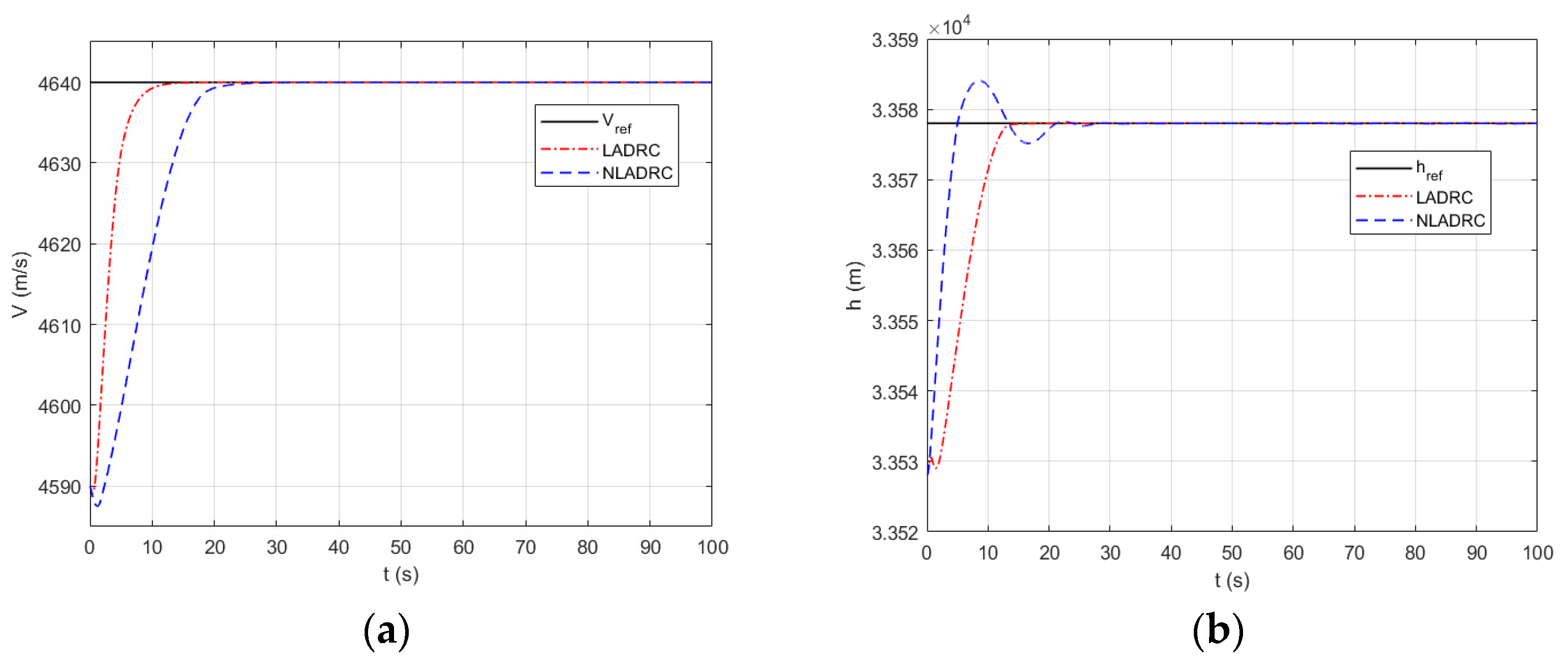
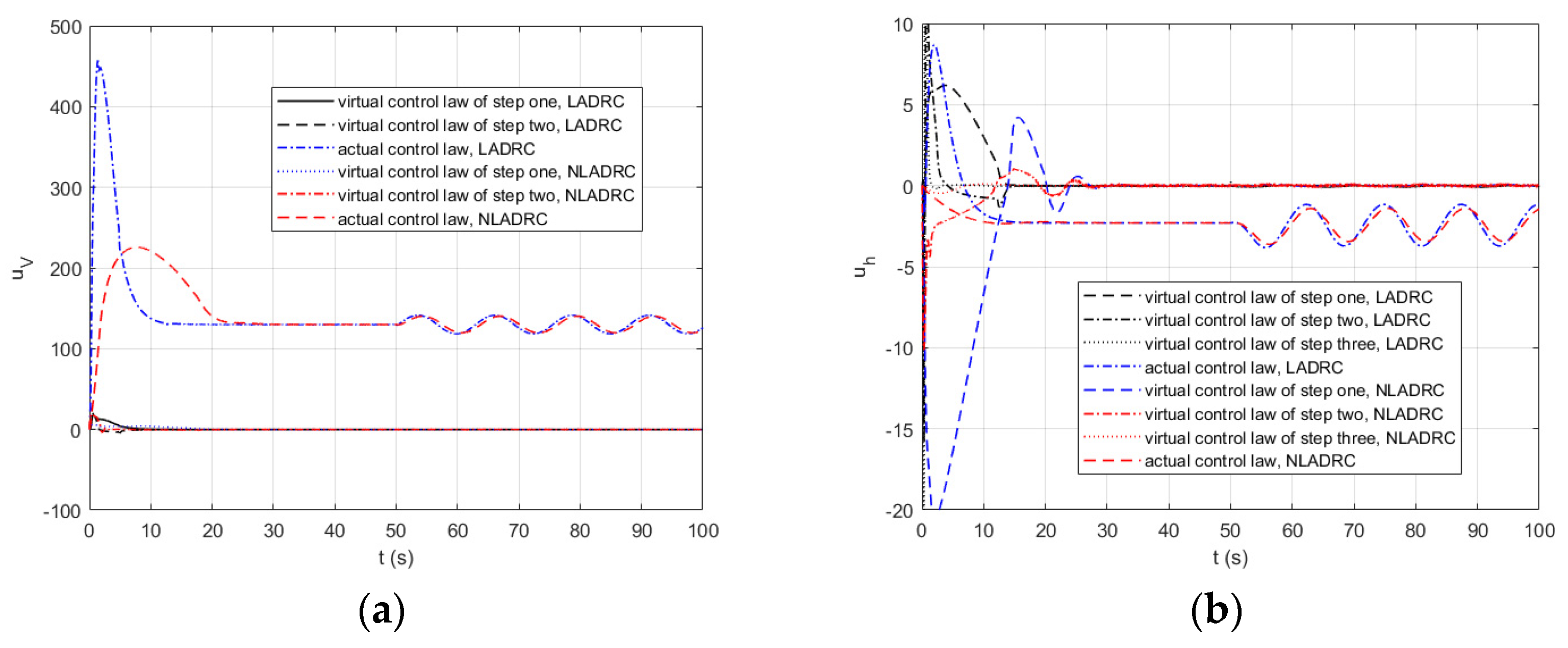
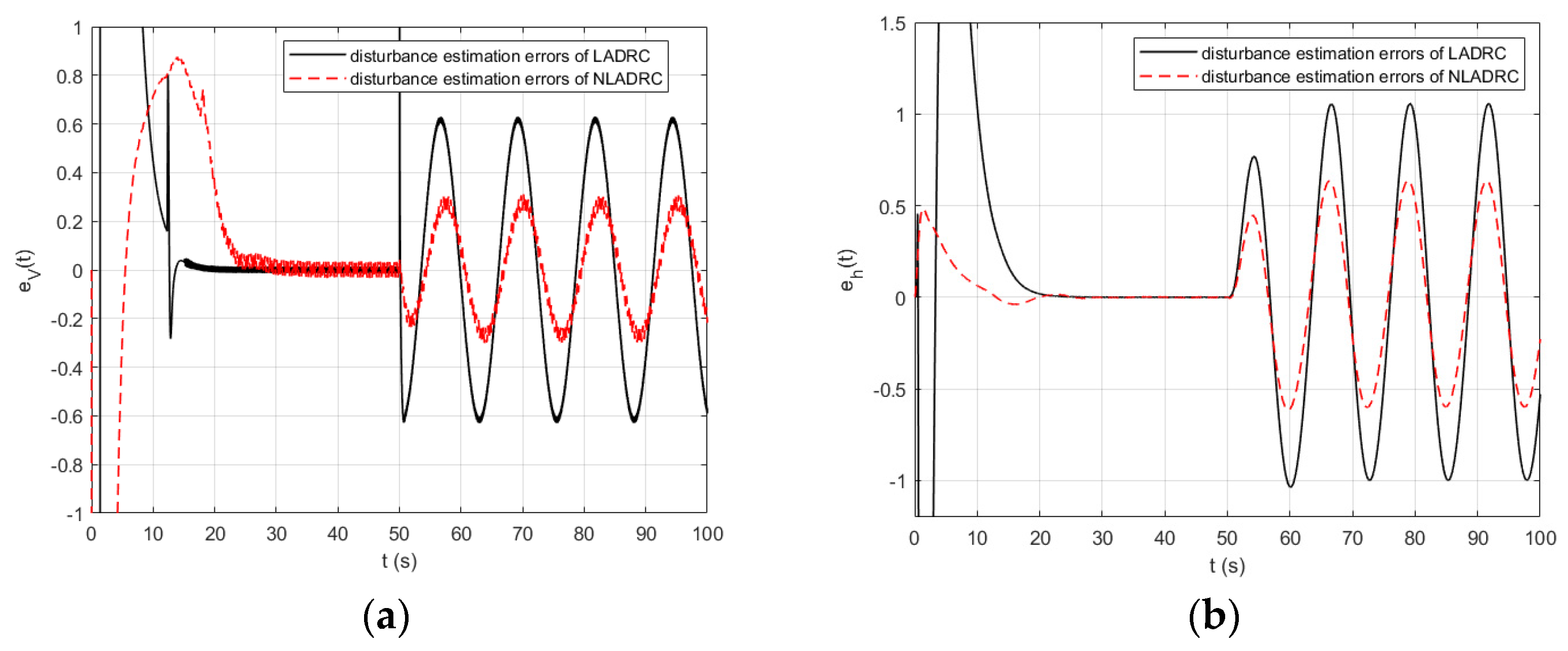
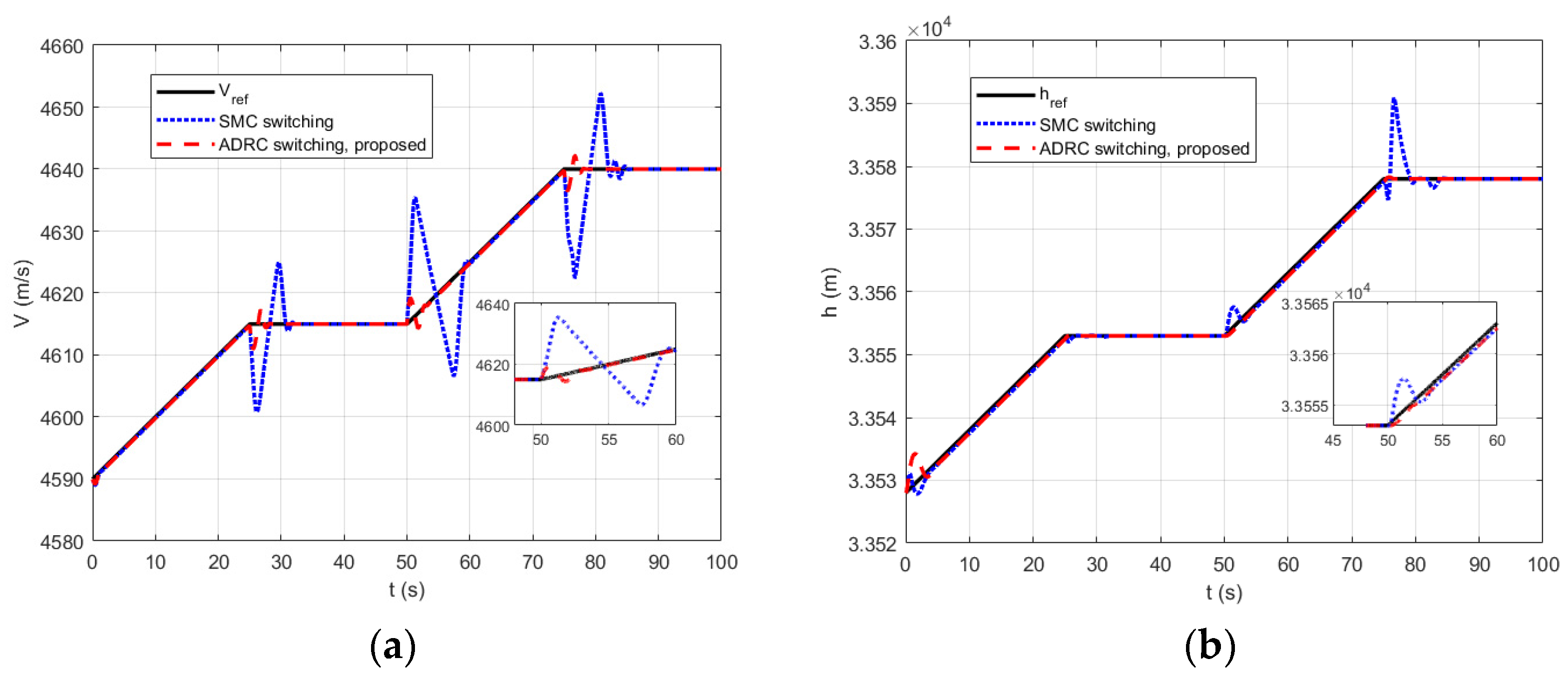
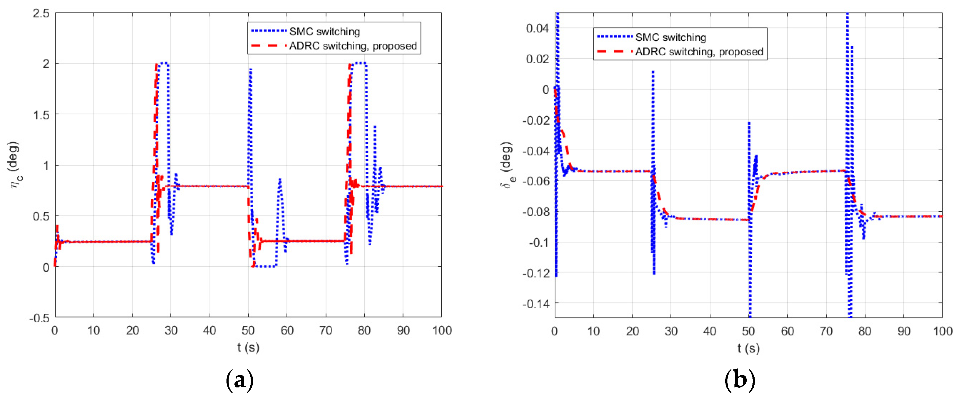
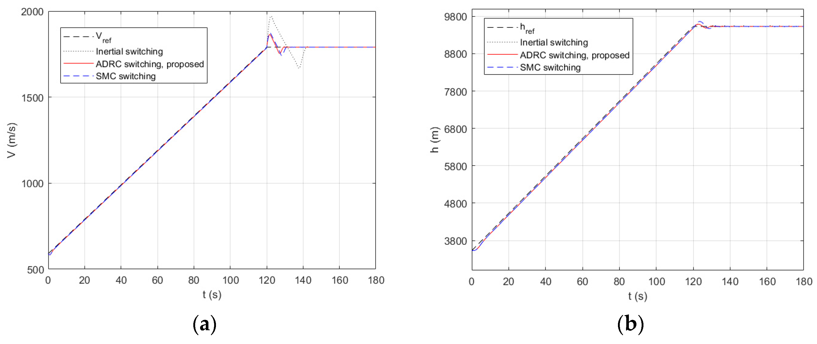
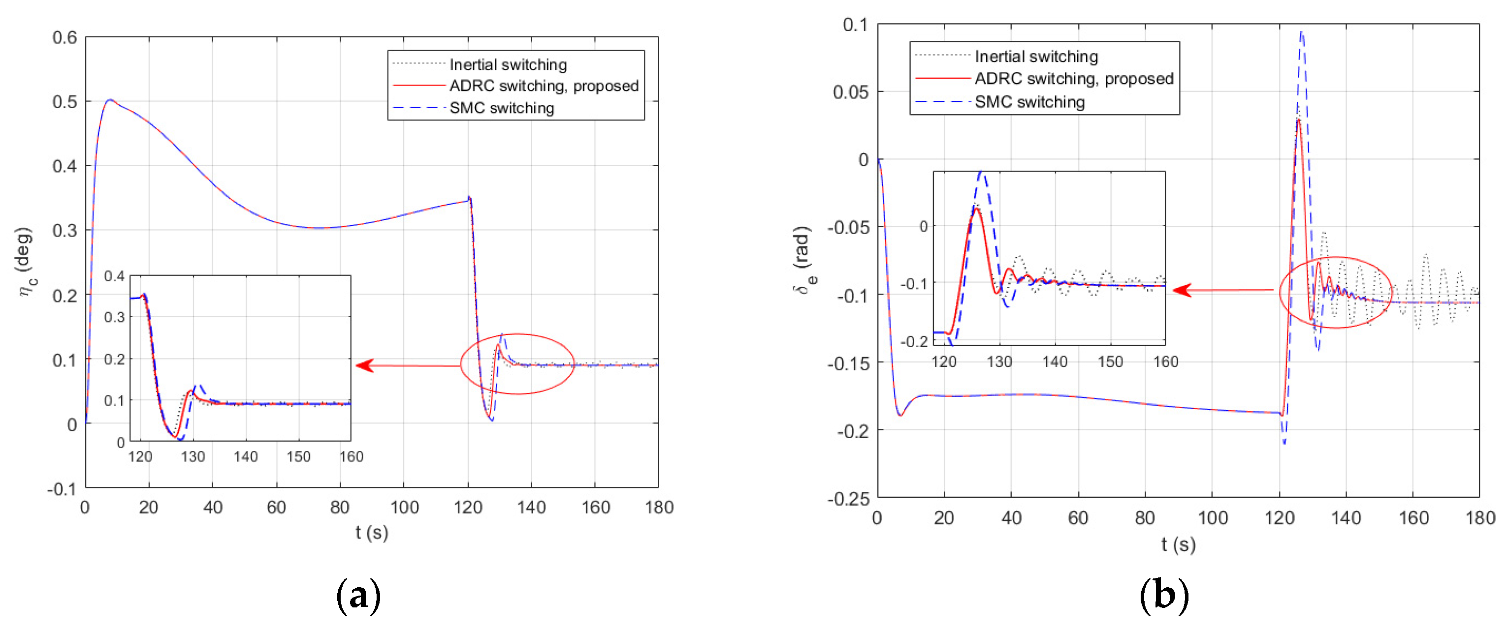
4.2. Multimodal Switching Simulation Analysis

Numerical simulations were executed to validate the efficiency of the linear/nonlinear active disturbance rejection switching control method.

Table 4. The initial flight condition for NMV.

States	Value	States	Value
$V(\mathrm{m}/\mathrm{s})$	4590	$m(\mathrm{k}\mathrm{g})$	50,200
$h(\mathrm{m})$	33,528	$I_{yy}(\mathrm{k}\mathrm{g}\cdot {\mathrm{m}}^2)$	8,466,900
$\gamma (\mathrm{r}\mathrm{a}\mathrm{d})$	0	$s({\mathrm{m}}^2)$	369
$\alpha (\mathrm{r}\mathrm{a}\mathrm{d})$	0	$\overline{c}(\mathrm{m})$	28
$q(\mathrm{r}\mathrm{a}\mathrm{d})$	0	$c_e$	0.0292

lists the initial flight condition at the initial simulation. Here, 20% parameter uncertainties were considered, that is, ${\Delta }_i=i_0\cdot 20\%\cdot \sin (\omega t)$, $i=m$, $s$, $\overline{c}$, $c_e$, $I_{yy}$, $C_L^{\alpha }$, $C_L^0$, $C_D^{{\alpha }^2}$, $C_D^{\alpha }$, $C_D^0$, $C_T^{\eta }$, $C_T^0$, $C_M^{\alpha ,{\alpha }^2}$, $C_M^{\alpha ,\alpha }$, $C_M^{\alpha ,0}$, $C_M^{q,{\alpha }^2}$, $C_M^{q,\alpha }$, $C_M^{q,0}$. The external disturbance was set as $d_V(t)=d_h(t)=0.5\cdot \sin (0.4t)$.

Case 1: Validate the effectiveness and disturbance rejection capability of the independent LADRC and NLADRC. In this case, considering aircraft cruise status, the reference trajectories of velocity and altitude were set as step signals of $V_{ref}=50(\mathrm{m}/\mathrm{s})$ and $h_{ref}=50(\mathrm{m})$. When the simulation time was $t=50(\mathrm{s})$, both parameter uncertainties and external disturbances were added. The simulation results are given in Figure 7, Figure 8 and Figure 9.

Figure 7 presents the tracking performance of velocity and altitude. It can be seen that the whole closed-loop system was stable by the action of LADRC or NLADRC. Compared with NLADRC, LADRC had the following advantages: a faster response speed, a shorter adjustment time, and a smoother transient response without overshoot. Figure 8 presents the virtual control laws and the actual control laws of the velocity and altitude subsystems. It can be seen that every step virtual control values could quickly converge to zero, the actual control values changed with the change in the parameter uncertainty and external disturbance, and dynamic compensation was realized for system uncertainty and external disturbance. Figure 9 presents the estimation errors of the total disturbance. It can be seen that the estimation error of NLADRC was less than that of LADRC, but NLADRC generated high-frequency oscillation, which was within the rational bounds of the estimation performance.

From the above analysis, it can be seen that both LADRC and NLADRC could quickly make the system stable. When an additional 20% parameter uncertainty and external disturbance were added, the system state was almost unaffected, which indicates that both LADRC and NLADRC can achieve stable flight control of NMVs and have strong disturbance rejection capability.

Case 2: Validate the effectiveness of LADRC/NLADRC switching control based on the type-2 fuzzy logic system. In this case, the reference trajectories of velocity and altitude were set as subsection function. When $t_1=t\in [0,25)$ and $t_3=t\in [50,75)$, the reference trajectories were set as ascent status. When $t_2=t\in [25,50)$ and $t_4=t\in [75,100]$, the reference trajectories were set as cruise status. From $t_1$ to $t_2$ then to $t_3$, the NMV mode changed from ascent to cruise then to ascent, and the winglet states changed from stretch out states to draw back states then to stretch out states. From $t_2$ to $t_3$ then to $t_4$, the NMV mode changed from cruise to ascent then to cruise, and the winglet states changed from draw back states to stretch out states then to draw back states. The parameters are given in

Table 5. The aerodynamic parameters at winglet switching time.

Winglet Switching Time	Aerodynamic Parameters
$t\in [25,30)$	$x\left(t\right)=x_1(t)e^{(-\lambda (t-25))}+x_2(t)(1-e^{(-\lambda (t-25))})$
$t\in [50,55)$	$x\left(t\right)=x_2(t)e^{(-\lambda (t-50))}+x_1(t)(1-e^{(-\lambda (t-50))})$
$t\in [75,80)$	$x\left(t\right)=x_1(t)e^{(-\lambda (t-75))}+x_2(t)(1-e^{(-\lambda (t-75))})$

. The simulation results are given in Figure 10, Figure 11, Figure 12 and Figure 13. In these images, “SMC switching” represents the algorithm proposed in [28].

Figure 10 presents the tracking performance of velocity and altitude for NMVs based on the multimodal switching control. It can be seen that the proposed control method could realize stable flight control for NMVs during modal switching. Whether from ascent mode to cruise mode (winglet from stretch out to draw back) or cruise mode to ascent mode (winglet from draw back to stretch out), the designed control strategy could achieve stable and smooth switching control for NMV. Furthermore, the ranges of oscillation amplitude generated by the switching method proposed in [28] were $\Delta V\approx [10,20]$ and $\Delta h\approx [5,15]$, and the switching transition time intervals were $t_V\approx [8,15]$ and $t_h\approx [4,8]$. Compared with the method proposed in [28], the ranges of oscillation amplitude generated by the switching method proposed in this paper were $\Delta V\approx [1,5]$ and $\Delta h\approx [1,3]$, and the switching transition time intervals were $t_V\approx [1,3]$ and $t_h\approx [1,3]$. Obviously, the switching method based on the type-2 fuzzy logic system had smaller oscillation amplitude, shorter transition time, and stronger disturbance rejection ability.

Figure 11 and Figure 12 present the actuator response and the change rules of the output weight of the type-2 fuzzy controller, respectively. It can be seen from Figure 11 that the switching method proposed in [28] generated a large number of high frequency oscillations. Compared to the method proposed in [28], the switching method proposed in this paper had smaller oscillation amplitude and smoother response curve. It can be seen from Figure 12 that NLADRC and LADRC were used in the ascent phase and cruise phase, respectively. Because there are always state errors and disturbance estimation errors in the whole switching process, the weight value cannot be taken as 0 or 1, but it still reflects the switching process of the controller. Figure 13 presents the responses of the angle of attack and the flight path angle. It can be seen that the switching method proposed in [28] caused a wide range of sudden changes for the attitude angle, which could easily lead to instability in the switching process. Compared to the method proposed in [28], the switching method proposed in this paper had smaller oscillation amplitude and smoother response curve, which can ensure stability in the switching process.

The above simulation analysis shows that the LADRC/NLADRC control method can realize stable tracking control for NMVs with a wide range of uncertain parameters and has strong disturbance rejection capability. Furthermore, the LADRC/NLADRC switching control method based on the type-2 fuzzy logic system can realize stable and smooth switching control for NMV multimodal switching. The proposed method has the advantages of small oscillation amplitude, shorter transition time, and stronger disturbance rejection capability.

Case 3: Validate the effectiveness of LADRC/NLADRC switching control during the transition from supersonic flight states to hypersonic flight states for NMVs. In this case, the reference trajectories of velocity and altitude were set as the following subsection function:

$$\left\{\begin{array}{l}V=10t+590,t<120\\ V=1790,t\ge 120\\ h=50t+3528,t<120\\ h=9528,t\ge 120\end{array}\right.$$

(41)

When $t\in [0,120)$, the winglet set as the stretch out states, the reference area $s=389({\mathrm{m}}^2)$ and the mean aerodynamic chord $\overline{c}=30(\mathrm{m})$, the aerodynamic parameters were given as $C_{i,sc}$. When $t\in [120,180]$, the winglet set as the draw back states, the reference area $s=369({\mathrm{m}}^2)$ and the mean aerodynamic chord $\overline{c}=28(\mathrm{m})$, the aerodynamic parameters were given as $C_{i,sh}$. When $t\in [120,130)$, the aerodynamic parameters were given as $x\left(t\right)=x_1(t)e^{(-\lambda (t-120))}+x_2(t)(1-e^{(-\lambda (t-120))})$. The simulation results are given in Figure 14, Figure 15, Figure 16, Figure 17 and Figure 18. In these images, “SMC switching” represents the algorithm proposed in [28].

Figure 14 and Figure 15 present the tracking performance of velocity and altitude for NMVs during the transition from supersonic flight states to hypersonic flight states. It can be seen that the proposed control method could realize stable switching control for NMVs during the transition from supersonic flight states to hypersonic flight states. Compared with the method proposed in [28] and the inertial switching method, the proposed switching control method has the advantages of smaller oscillation amplitude, smoother curve, and higher control accuracy. Figure 16 and Figure 17 present the actuator response and the change rules of the output weight of the type-2 fuzzy controller, respectively. As can be seen from the figure, NLADRC with high efficiency was used in the winglet stretch out states of the supersonic flight, and LADRC was used in the winglet draw back states of the hypersonic flight, that is, the switching method was from NLADRC to LADRC, mainly because the NLADRC method is prone to high-frequency oscillations when the parameters change, which is not conducive to the overall flight control requirements. When the transition from supersonic flight states to hypersonic flight states, the output weight of the type-2 fuzzy controller changed according to the parameter changes and converged to a steady-state value in a relatively short time. Figure 18 presents the responses of the angle of attack and the flight path angle. It can be seen that the method proposed in [28] and the inertial switching method caused large-range abrupt changes in the attitude angles and high-frequency oscillations during the switching process, which can easily lead to instability in the switching process. The proposed switching control method based on the type-2 fuzzy control system made the attitude angle change smaller and smoother, made the convergence time shorter, and improved the smoothness of the switching process.

5. Conclusions

In this paper, a novel linear/nonlinear active disturbance rejection switching control method for the longitudinal dynamical model of NMVs based on the type-2 fuzzy logic system is proposed. In order to obtain a practical control-oriented model, a large range of parameter uncertainty and external disturbance were considered. For the sake of enhancing the robustness of the system, both linear active disturbance rejection control (LADRC) and nonlinear active disturbance rejection control (NLADRC) were designed for the velocity and altitude subsystems of NMVs. Furthermore, a novel switching control strategy based on the interval type-2 fuzzy logic system was adopted to achieve multimodal switching control for winglet stretch out and draw back of NMVs. Finally, simulation and discussion results demonstrated that the proposed control method can realize stable and smooth switching control for NMVs. This paper provides new ideas for a cascade ADRC switching control method for a class of high-order coupled system and has high engineering application value.

References

1. Yang, J.; Li, S.; Sun, C.; Guo, L. Nonlinear Disturbance Observer Based Robust Flight Control for Airbreathing Hypersonic Vehicles. IEEE Trans. Aerosp. Electron. Syst. 2013, 49, 1263–1275. [Google Scholar] [CrossRef]
2. Sun, H.; Li, S.; Sun, C. Finite time integral sliding mode control of hypersonic vehicles. Nonlinear Dyn. 2013, 73, 229–244. [Google Scholar] [CrossRef]
3. Xu, B.; Zhang, Q.; Pan, Y. Neural network based dynamic surface control of hypersonic flight dynamics using small-gain theorem. Neurocomputing 2016, 173, 690–699. [Google Scholar] [CrossRef]
4. Xu, B.; Wang, D.; Zhang, Y.; Shi, Z. DOB-Based Neural Control of Flexible Hypersonic Flight Vehicle Considering Wind Effects. IEEE Trans. Ind. Electron. 2017, 64, 8676–8685. [Google Scholar] [CrossRef]
5. Bu, X.; He, G.; Ke, W. Tracking control of air-breathing hypersonic vehicles with non-affine dynamics via improved neural back-stepping design. ISA Trans. 2018, 75, 88–100. [Google Scholar] [CrossRef] [PubMed]
6. Gao, Z. Active disturbance rejection control: A paradigm shift in feedback control system design. In Proceedings of the 2006 American Control Conference, Minneapolis, MN, USA, 14–16 June 2006. [Google Scholar] [CrossRef]
7. Huang, Y.; Xue, W. Active disturbance rejection control: Methodology and theoretical analysis. ISA Trans. 2014, 53, 963–976. [Google Scholar] [CrossRef] [PubMed]
8. Guo, B.; Liu, J. Sliding mode control and active disturbance rejection control to the stabilization of one-dimensional Schrdinger equation subject to boundary control matched disturbance. Int. J. Robust Nonlinear Control 2015, 24, 2194–2212. [Google Scholar] [CrossRef] [Green Version]
9. Zhao, Z.; Guo, B. On active disturbance rejection control for nonlinear systems using time-varying gain. Eur. J. Control 2015, 23, 62–70. [Google Scholar] [CrossRef]
10. Aguilar, I.C.; Sira, R.H.; Acosta, J.A. Stability of active disturbance rejection control for uncertain systems: A Lyapunov perspective. Int. J. Robust Nonlinear Control 2017, 27, 4541–4553. [Google Scholar] [CrossRef]
11. Du, H.; Fan, Y.; Yan, J. Active Disturbance Rejection Control for Airbreathing Hypersonic Vehicle. Comput. Mod. 2013, 16, 1612–1622. [Google Scholar]
12. Tian, J.; Zhang, S.; Li, S. Active disturbance rejection control based robust output feedback autopilot design for airbreathing hypersonic vehicles. ISA Trans. 2018, 74, 45–59. [Google Scholar] [CrossRef] [PubMed]
13. Xu, Z.; Sun, C.; Yang, M.; Liu, Q. Active disturbance rejection control for hydraulic systems with full-state constraints and input saturation. IET Control Theory Appl. 2022, 16, 1127–1136. [Google Scholar] [CrossRef]
14. Yang, Z.; Yan, Z.; Lu, Y.; Wang, W.; Yu, L.; Geng, Y. Double DOF Strategy for Continuous-Wave Pulse Generator Based on Extended Kalman Filter and Adaptive Linear Active Disturbance Rejection Control. IEEE Trans. Power Electron. 2022, 37, 1382–1393. [Google Scholar] [CrossRef]
15. Bu, X.; Qi, Q. Fuzzy optimal tracking control of hypersonic flight vehicles via single-network adaptive critic design. IEEE Trans. Fuzzy Syst. 2022, 30, 270–278. [Google Scholar] [CrossRef]
16. Bu, X.; Qi, Q.; Jiang, B. A Simplified Finite-time Fuzzy Neural Controller with Prescribed Performance Applied to Waverider Aircraft. IEEE Trans. Fuzzy Syst. 2022, 30, 2529–2537. [Google Scholar] [CrossRef]
17. Zeghlache, S.; Kara, K.; Saigaa, D. Fault tolerant control based on interval type-2 fuzzy sliding mode controller for coaxial trirotor aircraft. ISA Trans. 2015, 59, 215–231. [Google Scholar] [CrossRef]
18. Erdal, K.; Reinaldo, M. Type-2 Fuzzy Logic Trajectory Tracking Control of Quadrotor VTOL Aircraft With Elliptic Membership Functions. IEEE/ASME Trans. Mechatron. 2017, 22, 339–348. [Google Scholar]
19. Wang, J.; Hu, L.; Chen, F.; Wen, C. Multiple-step fault estimation for interval type-II T-S fuzzy system of hypersonic vehicle with time-varying elevator faults. Int. J. Adv. Robot. Syst. 2017, 14, 1–17. [Google Scholar] [CrossRef] [Green Version]
20. Jiao, X.; Fidan, B.; Jiang, J.; Kamel, M. Type-2 fuzzy adaptive sliding mode control of hypersonic flight. Proc. Inst. Mech. Eng. 2019, 233, 2731–2744. [Google Scholar] [CrossRef]
21. Tao, X.; Yi, J.; Pu, Z.; Xiong, T. Robust Adaptive Tracking Control for Hypersonic Vehicle Based on Interval Type-2 Fuzzy Logic System and Small-Gain Approach. IEEE Trans. Cybern. 2021, 51, 2504–2517. [Google Scholar] [CrossRef]
22. Chen, F.; Hu, L.; Wen, C. Improved adaptive fault-tolerant control design for hypersonic vehicle based on interval type-2 T-S model. Int. J. Robust Nonlinear Control 2018, 28, 1097–1115. [Google Scholar] [CrossRef]
23. Yu, C.; Jiang, J.; Wang, S.; Han, B. Fixed-time adaptive general type-2 fuzzy logic control for air-breathing hypersonic vehicle. Trans. Inst. Meas. Control 2021, 43, 2143–2158. [Google Scholar] [CrossRef]
24. Huang, Y.; Sun, C.; Qian, C.; Wang, L. Linear parameter varying switching attitude control for a near space hypersonic vehicle withparametric uncertainties. Int. J. Syst. Sci. 2014, 46, 3019–3031. [Google Scholar] [CrossRef]
25. An, H.; Wu, Q.; Xia, H.; Wang, C.; Cao, X. Adaptive controller design for a switched model of air-breathing hypersonic vehicles. Nonlinear Dyn. 2018, 94, 1851–1866. [Google Scholar] [CrossRef]
26. Dou, L.; Gao, J.; Zong, Q.; Ding, Z. Modeling and switching control of air-breathing hypersonic vehicle with variable geometry inlet. J. Frankl. Inst. 2018, 355, 6904–6926. [Google Scholar] [CrossRef] [Green Version]
27. Ye, H.; Jiang, B. Adaptive Switching Control for Hypersonic Vehicle with Uncertain Control Direction. J. Frankl. Inst. 2020, 357, 8851–8869. [Google Scholar] [CrossRef]
28. Jiao, X.; Baris, F.; Jang, J.; Mohamed, K. Adaptive mode switching of hypersonic morphing aircraft based on type-2 TSK fuzzy sliding mode control. Sci. China Inf. Sci. 2015, 58, 1–15. [Google Scholar] [CrossRef] [Green Version]
29. Bolender, J.M.; Doman, D. Nonlinear longitudinal dynamical model of an air-breathing hypersonic vehicle. J. Spacecr. Rocket. 2007, 44, 374–387. [Google Scholar] [CrossRef]
30. Xu, W.; Li, Y.; Lv, M.; Pei, B. Modeling and switching adaptive control for nonlinear morphing aircraft considering actuator dynamics. Aerosp. Sci. Technol. 2022, 122, 107349.1–107349.17. [Google Scholar] [CrossRef]
31. Li, J.; Qi, X.; Xia, Y.; Gao, Z. On Linear/Nonlinear Active Disturbance Rejection Switching Control. Acta Autom. Sin. 2016, 42, 202–212. [Google Scholar]
32. Wu, Z.; Deng, C.; Wen, H. Fuzzy Linear/Nonlinear Active Disturbance Rejection Switching Control and Its Application. Acta Aeronaut. Astronaut. Sin. 2021, 42, 473–480. [Google Scholar]
Figure 1. Illustrations of typical NMV modes based on X-24B configuration.
Applsci 13 08255 g001
Figure 2. Block diagram of the ADRC for a multivariable coupling system.
Applsci 13 08255 g002
Figure 3. Three-dimensional graph of the Gaussian interval type-2 membership function.
Applsci 13 08255 g003
Figure 4. (a) The change rules of lift coefficient of the winglet from draw back to stretch out. (b) The change rules of lift coefficient of the winglet from stretch out to draw back.
Applsci 13 08255 g004
Figure 5. (a) The change rules of drag coefficient of the winglet from draw back to stretch out. (b) The change rules of drag coefficient of the winglet from stretch out to draw back.
Applsci 13 08255 g005
Figure 6. (a) The change rules of pitch moment coefficient of the winglet from draw back to stretch out. (b) The change rules of pitch moment coefficient when the winglet from stretch out to draw back.
Applsci 13 08255 g006
Figure 7. (a) Responses of velocity. (b) Responses of altitude.
Applsci 13 08255 g007
Figure 8. (a) Virtual control law and actual control law of the velocity subsystem. (b) Virtual control law and actual control law of the altitude subsystem.
Applsci 13 08255 g008
Figure 9. (a) Disturbance estimation errors of the velocity subsystem. (b) Disturbance estimation errors of the altitude subsystem.
Applsci 13 08255 g009
Figure 10. (a) Responses of velocity. (b) Responses of altitude.
Applsci 13 08255 g010
Figure 11. (a) Responses of the throttle setting. (b) Responses of the elevator deflection.
Applsci 13 08255 g011
Figure 12. (a) The output weight of the type-2 fuzzy controller of the velocity subsystem. (b) The output weight of the type-2 fuzzy controller of the altitude subsystem.
Applsci 13 08255 g012
Figure 13. (a) The angle of attack. (b) The flight path angle.
Applsci 13 08255 g013
Figure 14. (a) Responses of velocity. (b) Responses of altitude.
Applsci 13 08255 g014
Figure 15. (a) Tracking error of velocity. (b) Tracking error of altitude.
Applsci 13 08255 g015
Figure 16. (a) Responses of the throttle setting. (b) Responses of the elevator deflection.
Applsci 13 08255 g016
Figure 17. (a) The output weight of the type-2 fuzzy controller of the velocity subsystem. (b) The output weight of the type-2 fuzzy controller of the altitude subsystem.
Applsci 13 08255 g017
Figure 18. (a) The angle of attack. (b) The flight path angle.
Applsci 13 08255 g018