Mobile Charging Scheduling Approach for Wireless Rechargeable Sensor Networks Based on Multiple Discrete-Action Space Deep Q-Network

Abstract

Wireless energy transfer technology (WET)-enabled mobile charging provides an innovative strategy for energy replenishment in wireless rechargeable sensor networks (WRSNs), where the mobile charger (MC) can charge the sensors sequentially by WET according to the mobile charging scheduling scheme. Although there have been fruitful studies, they usually assume that all sensors will be charged fully once scheduled or charged to a fixed percentage determined by a charging upper threshold, resulting in low charging performance as they cannot adjust the charging operation on each sensor adaptively according to the real-time charging demands. To tackle this challenge, we first formulate the mobile charging scheduling as a joint mobile charging sequence scheduling and charging upper threshold control problem (JSSTC), where the charging upper threshold of each sensor can adjust adaptively. Then, we propose a novel multi-discrete action space deep Q-network approach for JSSTC (MDDRL-JSSTC), where MC is regarded as an agent exploring the environment. The state information observed by MC at each time step is encoded to construct a high-dimensional vector. Furthermore, a two-dimensional action is mapped to the charging destination of MC and the corresponding charging upper threshold at the next time step, using bidirectional gated recurrent units (Bi-GRU). Finally, we conduct a series of experiments to verify the superior performance of the proposed approach in prolonging the lifetime compared with the state-of-the-art approaches.

1. Introduction

As one of the basic supporting technologies of the Internet of Things, wireless sensor networks (WSNs) have attracted extensive research interest because they are widely used in many fields, including target monitoring, environmental monitoring, smart cities, smart medical care, industrial manufacturing, military fields [1], etc. However, energy constraints are a bottleneck for the development of WSNs, as existing sensors are all battery-powered and cannot achieve sustainable operation. The focus of early works is mostly on the sleep scheduling and network protocol scheduling [2,3,4]. Although the network lifetime was effectively prolonged, it did not fundamentally overcome the energy constraint problem.

The continuous development of wireless energy transfer technology (WET) brings opportunities to break through the bottleneck problem of energy constraint in WSN. Applying WET to WSNs, these networks with energy replenishment capability can be named wireless rechargeable sensor networks (WRSNs). Among the many WET-based charging schemes, employing a mobile charger (MC) equipped with a WET device to charge sensors wirelessly in the network is a promising approach. Mobile charging has high flexibility, controllability, and more cost-effective features, so it has received extensive attention.

Traditionally, mobile charging approaches are always divided into two categories: periodic charging and [5,6,7] on-demand charging [8,9,10,11]. Periodic charging is mostly used in scenarios where the environmental information rarely changes, including sensor position, energy consumption rate, moving speed, charging speed, etc. It is noted that when the environment state information changes with time, the periodic charging approach will not be able to find the optimal solution, resulting in more sensors failing in advance and deteriorating the charging performance of the network. However, on-demand charging can well balance the real-time change of sensor energy consumption and the adaptive adjustment of charging strategy, because MC charges the sensors according to their charging requests.

Although the existing works have made great progress in improving the charging performance, there are still some things that could be improved in both periodic and on-demand charging approaches. Thus, the above work can only give an approximate optimal charging strategy. Moreover, as the network scale increases, it is hard for the above work to solve the mobile charging problem quickly and reliably.

Deep reinforcement learning (DRL) can handle the mobile charging scheduling problem mentioned above, because DRL combines the ability of deep learning (DL) to perceive the environment and the ability of reinforcement learning (RL) to determine the charging decisions. Furthermore, compared with RL, DRL can deal with high-dimensional state space and action space and has stronger generalization ability. DRL can obtain the solution to the problem based on a small amount of prior experimental knowledge, which provides a solution to the increasingly complex mobile charging scheduling problem in WRSN. Currently, some studies have proposed deep reinforcement learning approaches for mobile charging schedules [12,13,14].

Existing studies based on deep reinforcement learning approaches have a common shortcoming. They all assume that each sensor would be fully charged or that all sensors would be charged to a fixed upper threshold. This will increase the risk of premature failure of the subsequent sensors with urgent charging demand. It is clear that the adaptive adjustment of the charging destination and the charging upper threshold according to the state of the network is more beneficial to prolonging the network lifetime. Therefore, inspired by the above studies, in this paper, we assume that each sensor can be charged partially and that the charging upper threshold can be adjusted adaptively, and we study the joint mobile charging sequence scheduling and charging upper threshold control problem (JSSTC). Correspondingly, we propose a novel multi-discrete action space deep Q-network approach for JSSTC (MDDRL-JSSTC).

The main contributions of the paper are summarized as follows.

(1)

The joint mobile charging sequence scheduling and charging upper threshold control problem (JSSTC) is studied in this paper. MC can adjust the charging upper threshold for each sensor adaptively according to the state information at each time step, where the time step is the time at which the charging decision is determined.

(2)

A bidirectional gated recurrent unit (Bi-GRU) is integrated in the Q-network, which guides the agent in determining the charging action of the next time step based on the past and future state information.

(3)

Simulation results show that the proposed method can effectively prolong the network lifetime compared to existing approaches.

The rest of the paper is organized as follows: The system model and problem formulation are introduced in Section 2. The details of MDDRL-JSSTC are described in Section 3. The charging performance of the proposed approach is evaluated in Section 4. The discussion of the results is given in Section 5. Conclusions and future work are presented in Section 6.

2. Related Work

2.1. Periodic Charging and On-Demand Charging Scheduling Approaches

Periodic charging and on-demand charging scheduling approaches are the focus of mobile charging in WRSN in the early stage. For example, in [5], Shi et al. proposed an optimization approach that maximized the ratio of vacation time to the cycle time of an MC via periodic charging. Wang et al. [6] studied the mobile charging trajectory optimization problem based on the background of unbalanced energy consumption speed of sensors in the network and limited MC capacity, by transforming it to a traveling salesman problem. In our previous works, Li et al. [7] proposed an improved quantum-behaved particle swarm optimization approach for the mobile charging sequence scheduling to guarantee the sensing coverage quality of the network. Lin et al. [8] proposed a game theoretical collaborative on-demand charging scheduling approach to increase overall usage efficiency using the Nash Equilibrium. In [9], He et al. proposed an approach, named uncomplicated and efficient nearest-job-next with preemption (NJNP), to make the charging decision for MC according to the distance between the position of the sensor in the candidate charging queue and the MC. Based on NJNP, in [10], Lin et al. proposed a temporal-spatial real-time charging scheduling approach (TSCA) by considering the expected failure time of the sensor and the distance from the MC comprehensively. In [11], A. Tomar et al. proposed a fuzzy logic-based on-demand algorithm to determine the charging schedule of the energy-hungry nodes for multiple mobile chargers.

2.2. Mobile Charging Scheduling Approaches Based on DRL

As the network becomes more and more complex, in recent years, some works have modeled the mobile charging scheduling problem as a Markov decision process (MDP) and adopted deep reinforcement learning approaches. For example, in [12], Cao proposed a deep reinforcement learning approach for an on-demand charging scheme, which aims to maximize the total reward on each charging tour. Yang et al. proposed an actor-critic reinforcement learning approach for a dynamic charging scheme to prolong the network lifetime [13]. In [14], Bui et al. proposed a deep reinforcement learning-based adaptive charging policy for WRSNs to maximize the lifetime, while ensuring that all targets in the network are monitored. To highlight the differences between this study and existing ones, a comprehensive comparison is summarized in Table 1.

Table 1. A comparison between existing studies and this study.

	Periodic Charging			On-Demand Charging			DRL-Based Approaches
	[5]	[6]	[7]	[8]	[9]	[10]	[12]	[13]	[14]	This Work
Is the MC involved?	√	√	√	√	√	√	√	√	√	√
Are sensors charged with WET?	√	√	√	√	√	√	√	√	√	√
Are energy consumption rates dynamic?					√	√	√	√	√	√
Is charging upper threshold adaptively adjusted?										√
Is the energy capacity of MC limited?		√					√	√	√	√
Is there charging sequence scheduling?	√	√	√	√	√	√	√	√	√	√
Is there a joint optimization?						√		√		√
Are there multiple action spaces?										√

3. System Model and Problem Formulation

3.1. System Model

Figure 1 describes the network model of WRSN, which mainly consists of four components: n sensors, a charging service station, an MC, and a base station. Four units are equipped on each sensor, including a sensing unit, a wireless energy receiver, a processing unit, and a transceiver unit. Each sensor has the same energy capacity $E_{sn}^{max}$; the set of the sensors is defined as $SN=\{{sn}_1,{sn}_2,\dots ,{sn}_n\}$. The position of each sensor is $p_{{sn}_i}=(x_i,y_i)$, and the remaining energy of each sensor is $E_{{sn}_i}^r$, $i=\{\mathrm{1,2},\dots ,n\}$, where i is the integral index of the sensors. The position of charging service station is $p_d=(x_d,y_d)$; the distance between any two charging destinations of the MC, including the sensors and the charging service station, is $d_{i,j}$, where $d_{i,j}=\sqrt[2]{{{(x}_i-x_j)}^2+{{(y}_i-y_j)}^2}$.

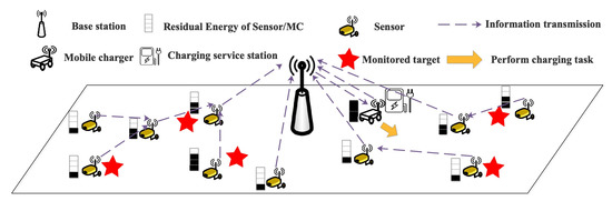
Figure 1. Network model.

A wireless energy transfer module is equipped on the MC, which can transfer energy to the sensors and move freely in the network without obstacles. If the remaining energy of the MC is not enough to continue the charging task, it needs to return to the charging service station to change its battery. The process of starting from the charging service station, performing the charging task in the network, and returning to the charging service station to replace the battery can be regarded as a charging tour of MC. Furthermore, the sensor and the MC must communicate with the base station periodically. The MC transmits its own location and remaining energy information and obtains the charging policy from the base station. The sensors adopt classic MAC and routing protocols [15] and transmit their monitored information to the base station in a multi-hop communication via the path with minimum energy consumption.

3.2. The Models of Energy Consumption and Charging

The energy of the sensor is mainly consumed in information transmission and receiving. The sensor energy consumption rate is denoted as $e_{{sn}_i}^c,i=\{\mathrm{1,2},\dots ,n\}$, where i is the integral index of the sensors. We adopt the same energy consumption model as [5], which estimates the $e_{{sn}_i}^c$ with the base station using the residual energy profile of the sensor. The initial remaining energy of sensors is $E_{{sn}_i}^0$. Then, the energy of the MC is mainly consumed in communication and moving and charging the sensor. In particular, the energy consumed in communication can be ignored compared to the other parts. $e_{MC}^m$ is the energy consumed to move a unit distance. $p_{MC}^c$ and $v_{MC}$ are the charging rate and moving speed of MC. $E_{MC}^{max}$ is the MC energy capacity, and $E_{MC}^r$ is the MC remaining energy. $E_{MC}^{min}$ is the minimum remaining energy threshold for MC to return to the charging service station to replace the battery. When the remaining energy of MC reaches the threshold, the charging task should be terminated in advance.

In this paper, we assume that the charging upper threshold of each sensor can be adjusted adaptively and ask the MC to charge the sensor via a one-to-one charging model with magnetic resonant coupling [16]. Therefore, when the MC performs the charging task, it mainly consists of three phases: (1) moving to the charging destination, (2) charging the sensor to its charging upper threshold, and (3) returning to the charging service station.

Therefore, the moving time and the energy consumed between the two charging destinations are obtained by

$$t_{MC}^m=\frac{d_{i,j}}{v_{MC}},$$

(1)

$$E_{MC}^m=d_{i,j}\cdot e_{MC}^m.$$

(2)

The time to charge a sensor is determined by

$$t_{MC}^c=\frac{{\varsigma }_i·(E_{sn}^{max}-{\tilde{E}}_{{sn}_i}^r)}{p_{MC}^c-e_{{sn}_i}^c},$$

(3)

where ${\varsigma }_i$ represents the charging upper threshold of ${sn}_i$, and ${\tilde{E}}_{{sn}_i}^r$ is the remaining energy before the charging action is performed. During one charging operation, the total energy consumed by MC is obtained by (4), which consists of moving to the sensor and charging.

$$E_{MC}^T=d_{i,j}\cdot e_{MC}^m+{\varsigma }_i\cdot {(E}_{sn}^{max}-{\tilde{E}}_{{sn}_i}^r).$$

(4)

Furthermore, in one charging operation, the total energy consumed by sensor ${sn}_i$ is

$$E_{{sn}_i}^T=e_{{sn}_i}^c\cdot \left(t_{MC}^m+t_{MC}^c\right).$$

(5)

3.3. Problem Formulation

In this paper, MC is assumed to adjust the charging upper threshold adaptively for each sensor according to the charging demand, and the charging operation is triggered at a time step. The index of the time step is defined as k; the maximum time step is K; and the charging policy is defined as $\mathsf{\Pi }$, where $\mathsf{\Pi }=\{{\mathsf{\Lambda }}_1,\dots ,{\mathsf{\Lambda }}_k,\dots ,{\mathsf{\Lambda }}_K\}$. ${\mathsf{\Lambda }}_k$ represents the charging operation at k-th time step, which includes the charging destination of MC ${\vartheta }_k$ and the charging upper threshold ${\varsigma }_k$, described as ${\mathsf{\Lambda }}_k=({\vartheta }_k,{\varsigma }_k)$. For the convenience of statistics, we define the index of the charging service station as 0. Thus, ${\vartheta }_k=\{\mathrm{0,1},\dots ,n\}$.

In theory, the network lifetime can be prolonged to infinity with one or multiple MC. However, the energy consumption rate distribution of sensors in the network is uneven, and the aging of the energy module of the sensors will hinder the continued prolonging of the lifetime. Therefore, inspired by [17,18,19], we define the network lifetime such that when the number of failed sensors reaches the total number of $\omega \%$, the number of failed sensors is defined as $n_d$, and the network lifetime is described as $T_{life}$. Then, the JSSTC problem is formulated as

$$\begin{array}{cc}max& T_{life}\left(\mathsf{\Pi }\right)\\ s.t.& \begin{array}{cc}C1:& {\vartheta }_k=\left\{\mathrm{0,1},\dots ,n\right\},k=\left\{1,\dots ,K\right\},n,K\in {\mathit{N}}^{\ast }\\ C2:& {\varsigma }_k=\{\mathrm{0.1,0.2},\dots ,1\},k=\left\{1,\dots ,K\right\},K\in {\mathit{N}}^{\ast }\\ \begin{array}{c}C3:\\ C4:\\ \begin{array}{c}C5:\\ C6:\end{array}\end{array}& \begin{array}{c}0{\le E}_{{sn}_i}^r\le E_{sn}^{max},\hfill \\ {E_{MC}^{min}\le E}_{MC}^r\le E_{MC}^{max}\\ \begin{array}{c}{n}_d/n\le \omega \%\\ T_{life}\left(\mathsf{\Pi }\right)\le T_{target}\end{array}\end{array}\end{array}\end{array}$$

(6)

where C1 and C2 represent the value ranges of the charging decision. C3 and C4 are the physical constraints of the sensors and MC. C5 and C6 indicate that the ratio of failed sensors to the total number of sensors and the network lifetime should not exceed the preset threshold.

4. The Details of MMDRL-JSSTC

In this paper, the main purpose is that MC can adaptively adjust the charging sequence and the charging upper threshold according to system state information to prolong the network lifetime. The deep reinforcement learning approaches in existing works will not be able to address this problem. Therefore, a multi-dimensional discrete action space deep reinforcement learning approach is proposed for JSSTC (MMDRL-JSSTC).

4.1. Formulation of MMDRL-JSSTC

The MC is regarded as an agent that explores the WRSN and obtains observation information, extracts the environment information based on deep learning, and predicts the action to be performed in the next time step. Then, MC interacts with the environment based on the action predicted by deep learning. At any time step, the environment gives feedback based on the actions performed by the MC, which is defined as a reward. Figure 2 shows the flow chart of making charging decisions based on the DRL. The exploration process can be described by the tuple $\{S,\mathcal{A},R,S^{\prime }\}$, where $S$ is the state space of the system, $\mathcal{A}$ is the action space, $R$ is the reward feedbacked by the environment, and $S^{\prime }$ is the new state space after the MC performing the action. The details of the state information, action, policy, and reward are described below.

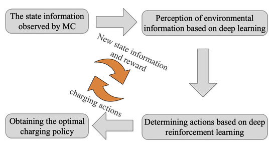
Figure 2. The flowchart of making charging decisions based on the DRL.

(1)

State.

The state information of this paper mainly consists of three parts, including the state of the sensors, MC, and the charging service station, described with $s\left(k\right)=\left(s_{sn}\right(k),s_{MC}(k),s_d(k\left)\right)$, which can help the MC determine the charging destination. The state information of each sensor is described with a tuple $s_{{sn}_i}\left(k\right)=(x_{{sn}_i},y_{{sn}_i},e_{{sn}_i}^c,E_{{sn}_i}^r,E_{sn}^{MAX})$; the state information of MC is described with $s_{MC}\left(k\right)=(x_{MC},y_{MC},e_{MC}^m,p_{MC}^c,E_{MC}^{max},E_{MC}^{min},E_{MC}^r)$; and the state information of charging service station is described with $s_d\left(k\right)=(x_d,y_d)$. The elements in the state information can be divided into static elements and dynamic elements. Therefore, in the above state information, $e_{{sn}_i}^c$, $E_{{sn}_i}^r$, $x_{MC}$, $y_{MC},$ and $E_{MC}^r$ are dynamic elements; the others are static.

(2)

Action.

We define that at any time step, the action $a\left(k\right)$ consists of discrete action pairs, which are the charging destination at next time step $a_{\vartheta }\left(k\right)$ and the correspond ding upper threshold $a_{\varsigma }\left(k\right)$, described with $a\left(k\right)=(a_{\vartheta }\left(k\right),a_{\varsigma }(k\left)\right)$. For the convenience of sorting, we assume that the index of the charging service station is 0. The MC needs to start from the charging service station and return to the charging service station to replace the battery. Therefore, the action $a_{\vartheta }\left(k\right)$ determined at time step k is an integer number ${a_{\vartheta }\left(k\right)\in \mathcal{A}}_{\vartheta }=\{\mathrm{0,1},\dots ,n\}$, and the action $a_{\varsigma }\left(k\right)$ determined at time step k is a float number $a_{\varsigma }\left(k\right)\in {\mathcal{A}}_{\varsigma }=\{\mathrm{0.1,0.2},\dots ,1\}$, described in Figure 3.

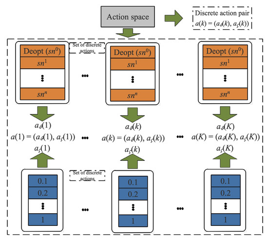
Figure 3. The action description of JSSTC.

(3)

Transition.

After the MC performs the charging action, the state of the network will change from $s\left(k\right)$ to $s(k+1)$. The energy consumption of the MC and the sensors can be obtained by Equations (4) and (5). It should be noted that MC can only observe the updated state information, and the underlying process is simulated in the base station.

(4)

Reward.

We utilize $r\left(s\right(k),a(k\left)\right)$ to describe the reward the agent gets after performing action $a\left(k\right)$ at state $s\left(k\right)$. Since the main purpose of this paper is to maximize the survival time of the network before the termination condition is met, this is equivalent to maximizing the duration of MC performing charging tasks. The charging task performed by MC includes charging and moving. Therefore, the sum of the moving time and the charging time corresponding to each time step is regarded as the reward of MC, which can be obtained by (1) and (3). In addition, the increased number of failed sensors due to charging decision will worsen the charging performance. Thus, we regard the number of new failed sensors as a penalty. Therefore, the reward $r\left(s\right(k),a(k\left)\right)$ is obtained by

$$r\left(s(k),a(k)\right)=t_{MC}^m\left(k\right)+t_{MC}^c\left(k\right)-\varphi \cdot \left(n_d\left(k\right)-n_d(k-1)\right),$$

(7)

where $\varphi$ is the penalty coefficient.

(5)

Policy.

When the test environment is terminated, all the charging actions performed by the MC during the charging process will compose a charging policy, described with $a=\mathsf{\Pi }\left(S\right)$, where $\mathsf{\Pi }=\{{\mathsf{\Lambda }}_1,\dots ,{\mathsf{\Lambda }}_k,\dots ,{\mathsf{\Lambda }}_K\}$, and ${\mathsf{\Lambda }}_k=({\vartheta }_k,{\varsigma }_k)$. Let ${a_{\vartheta }\left(k\right)=\vartheta }_k$ and ${a_{\varsigma }\left(k\right)=\varsigma }_k$, and $\mathsf{\Pi }:S\mapsto P\left(\mathcal{A}\right)$, where $P\left(\mathcal{A}\right)\in \left[\mathrm{0,1}\right]$. In particular, the main purpose of MC is to obtain an optimal charging policy to maximize the cumulative reward.

A scheduling example of JSSTC is shown in Figure 4. A charging trajectory can be described with $\left\{s\right(0),a\left(0\right),\dots ,s(k),a\left(k\right),\dots ,s(K-1),a\left(K-1\right),s(K\left)\right\}$, and the discounted cumulated reward is obtained by

$$R\left(\mathsf{\Pi }\right)={\displaystyle {\sum }_{k=0}^K}{{\rm Y}}^k\cdot r\left(s\left(k\right),a\left(k\right)\right),$$

(8)

where $s\left(k\right)\in S$, $a\left(k\right)\in \mathcal{A}$.

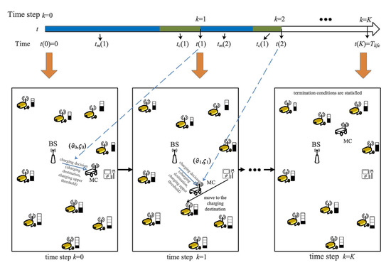
Figure 4. A scheduling example of JSSTC.

To effectively shorten the training time and teach the agent to avoid the meaningless exploration, some constraints are given as follows:

• The MC can visit any position in the network when its remaining energy of MC is greater than $E_{MC}^{min}$ and when its remaining energy reaches $E_{MC}^{min}$, it will terminate the current charging operation and return the charging service station to replace the battery;
• All sensors with charging demand greater than 0 can be selected as the next charging destination;
• If the remaining energy of the sensors is 0, it will not be accessed by MC;
• Two adjacent time steps cannot choose the same charging destination.

4.2. The Details of MDDRL-JSSTC

The training process of MDDRL-JSSTC is shown in Algorithm 1, and its structure is shown in Figure 5. The core framework of MDDRL-JSSTC is the deep Q-network (DQN); therefore, the parameterized Q-network and parameterized target Q-network can be defined as $Q\left(s\right(k),a(k);\theta )$ and $Q\left(s\right(k+1),a(k+1);\theta \prime )$. The convolutional neural network (CNN) is widely utilized as Q-network in DQN because of its excellent nonlinear mapping ability.

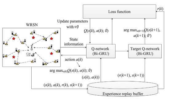
Figure 5. The structure of MMDRL-JSSTC.

In this paper, the charging sequence and charging upper threshold included in the charging decision have complex time characteristics. CNN lacks the ability to store time-series information and cannot predict future decisions based on historical information. The recurrent neural network (RNN) has good information memory ability, and the input of its hidden layer is not only related to the output of the previous layer but also related to the output of this layer in the previous layer of time step. Therefore, RNN accurately represents the complex temporal correlation between the current input sequence and the past information.

However, traditional RNNs have a drawback that they can only store short-term temporal memories. When too long a temporal series is an input in RNN, its gradient will explode or disappear, making the neural network invalid. The gated recurrent unit (GRU) is a variant of RNN which can better capture the dependencies of large intervals in temporal data, thus effectively alleviating the problems of gradient explosion and gradient disappearance. The input and output structure of GRU is the same as that of traditional RNN, mainly composed of four parts, the input at the k-th time step $x\left(k\right)$, the hidden layer state at k − 1 time step $h(k-1)$, the output at the k-th time step $y\left(k\right)$, and the hidden layer state transferred to the next time step $h\left(k\right)$.

The structure of the GRU is shown at the top of Figure 6. It mainly includes two gates: the reset gate and the update gate. The reset gate determines how much memory is saved and resets, and the update gate determines how much memory is retained to be updated to the current gate unit. At any time step, the GRU is updated based on the following:

$$u\left(k\right)=\sigma \left(w_u\cdot \left[h\left(k-1\right),x\left(k\right)\right]\right),$$

(9)

$$r\left(k\right)=\sigma \left(w_r\cdot \left[h\left(k-1\right),x\left(k\right)\right]\right),$$

(10)

$$\tilde{h}\left(k\right)=\tanh \left(w_h\cdot \left[r\left(k\right)\ast h\left(k-1\right),x\left(k\right)\right]\right),$$

(11)

$$h\left(k\right)=\left(1-u\left(k\right)\right)\ast h\left(k-1\right)+u\left(k\right)\ast \tilde{h}\left(k\right),$$

(12)

where $\sigma$ is the sigmoid function, described as $\sigma =1/(1+e^{-x})$. $\sigma$ can convert the data into a value from 0 to 1 and then act as a gate signal. $\mathrm{t}\mathrm{a}\mathrm{n}\mathrm{h}$ is the activation function, expressed as $\mathrm{t}\mathrm{a}\mathrm{n}\mathrm{h}={{(e}^x-e}^{-x})/({(e}^x+e^{-x})$. $\mathrm{t}\mathrm{a}\mathrm{n}\mathrm{h}$ can scale the data to the range −1 to 1. Furthermore, $w_u$, $w_r$, and $w_h$ are the weights that need to be updated, respectively.

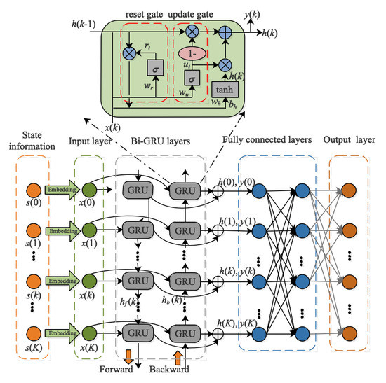
Figure 6. The structure of the Q-network in MMDRL-JSSTC.

Since the charging decision at any time step in this paper includes the charging destination and the corresponding charging upper threshold, it can be analyzed that both the past and the future charging decisions impact the current charging decision. To find a charging policy that maximizes the network lifetime, we introduce the bidirectional gated recurrent unit (Bi-GRU) in Q-network, which can predict the charging decision of the current time step based on historical and future information. Bi-GRU consists of a forward and backward GRU, as described in Figure 6. At any time step, the outputs of forward GRU and backward GRU are $h_f\left(k\right)$ and $h_b\left(k\right)$, respectively.

The process of obtaining the Q value in MDDRL-JSSTC is briefly described as follows:

(1)

The state information of any time step $s\left(k\right)$ is embedded to obtain a high-dimensional vector, and this vector is utilized as the input of Bi-GRU, denoted as $x\left(k\right)$;

(2)

After inputting the input information to Bi-GRU, the hidden state information $h\left(k\right)$ and output information $y\left(k\right)$ of any time step will be obtained, where the hidden state information is spliced by forward hidden state information and backward hidden state information, expressed as $h\left(k\right)=h_f\left(k\right)\oplus h_b\left(k\right)$;

(3)

Two fully connected layers are connected behind the Bi-GRU layer and then obtain the Q value.

It should be noted that because the actions performed by MC at any time step are two-dimensional, the Q value here is a two-dimensional list. Furthermore, the weights mentioned above are included in the $\theta$ and $\theta \prime$, and the specific training process will be briefly described as follows.

In MMDRL-JSSTC, the action value function is defined as $Q^{\mathsf{\Pi }}(s,a)$. The action value at k-th time step is obtained by

$$Q^{\mathsf{\Pi }}\left(s\left(k\right),a\left(k\right)\right)={\mathbb{E}}_{\mathsf{\Pi }}\left[{\sum }_{k=0}^K{\gamma }^{k}r\left(k\right)|s\left(k\right),a\left(k\right)=a_{\vartheta }\left(k\right),a_{\varsigma }\left(k\right)\right],$$

(13)

The action value function is updated according to the Bellman optimal equation, which can be expressed as

$$\begin{gathered} Q^{\mathsf{\Pi }}\left(s\left(k\right),a\left(k\right)\right)\leftarrow Q^{\mathsf{\Pi }}\left(s\left(k\right),a\left(k\right)\right)+ \\ \alpha \cdot \left[r+\gamma \cdot {max}_{a\left(k+1\right)}{Q}^{\mathsf{\Pi }}\left(s\left(k+1\right),a\left(k+1\right)\right)-Q^{\mathsf{\Pi }}\left(s\left(k\right),a\left(k\right)\right)\right] \end{gathered}$$

(14)

Q-network is updated by minimizing the loss function $L_i\left({\theta }_i\right)$

$$L_i({\theta }_i)={\mathbb{E}}_{s\left(k\right),a\left(k\right)~\rho \left(\cdot \right)}[{(y_j-Q^{\mathsf{\Pi }}\left(s\left(k\right),a\left(k\right);\theta \right))}^2],$$

(15)

where $a\left(k\right)~\rho \left(\cdot \right)$ represents the probability distribution of the action, and $y_j$ is

$$y(j)={\mathbb{E}}_{s\left(k+1\right)}\left[r_j+\gamma \cdot {max}_{a\left(k+1\right)}{Q}^{\mathsf{\Pi }}\left(s\left(k+1\right),a\left(k+1\right);{\theta }^{\prime }\right)\right].$$

(16)

The gradient of the loss function is defined as

$$\begin{gathered} {\nabla }_{{\theta }_i}{L}_i\left({\theta }_i\right)={\mathbb{E}}_{s\left(k\right),a\left(k\right)~\rho \left(\cdot \right);s\left(k+1\right)}\left[\right(r+\gamma \cdot {max}_{a^{\prime }}Q\left(s\left(k+1\right),a\left(k+1\right);{\theta }_{i-1}\right)- \\ Q(s\left(k\right),a\left(k\right);{\theta }_i)\cdot {\nabla }_{{\theta }_i}Q(s\left(k\right),a\left(k\right);{\theta }_i)\left)\right]. \end{gathered}$$

(17)

Algorithm 1 MDDRL-JSSTC

Input: Input the state information s, the maximum number of episode is $N_e$, maximum training step in one episode is K, the target network parameter update interval is $N_u$-step, discount factor $\gamma$

Output: $\theta$ and ${\theta }^{\prime }$

1. Initialization: Initialize the capacity of experience replay buffer $\mathbb{B}$ to $\mathsf{\Xi }$, initialize the weight of Q-network $\theta$ randomly, ${\theta }^{\prime }⟵\theta$

2.    for episode = 1 to $N_e$ do

3.       Initialize the network environment

4.       for k = 1 to K do

5.          Select an action $a_{\vartheta }\left(k\right)$ from ${\mathcal{A}}_{\vartheta },$ based on $\epsilon$-greedy at k-th time step

6.          Select an action $a_{\varsigma }\left(k\right)$ from ${\mathcal{A}}_{\varsigma },$ based on $\epsilon$-greedy at k-th time step

7.          Combine $a_{\vartheta }\left(k\right)$ and $a_{\varsigma }\left(k\right)$ to an action pair $a\left(k\right)=(a_{\vartheta }\left(k\right),a_{\varsigma }\left(k\right))$

8.          $\epsilon =\epsilon -∆\epsilon$

9.          Perform the action $a\left(k\right)$ on the environment, the environment feedback a reward $r\left(k\right)$, and a new state $s\left(k+1\right)$.

10.        Save the interaction process as tuple $\{s\left(k\right),a\left(k\right),r\left(k\right),s\left(k+1\right)\}$, and store it in $\mathbb{B}$

11.        Repeat performing 5–10

12.        Sample $\{s\left(j\right),a\left(j\right),r\left(j\right),s\left(j+1\right)\}$ randomly from minibatch $\mathsf{\Gamma }$

13.        if any conditions in (6) is not satisfied at j + 1-th time step

$\hspace{1em}\hspace{1em}\hspace{1em}\hspace{1em}\hspace{0.17em}\hspace{1em}\hspace{1em}\hspace{1em}\hspace{1em}y\left(j\right)=r\left(j\right)$

break.

14.        else

15.          Obtain the two-dimensional action value $y_{\vartheta }\left(j\right)$ and $y_{\varsigma }\left(j\right)$ with (14)

Update the parameters via (18)

16.        end if

17.        Update the parameter of target network with ${\theta }^{\prime }⟵\theta$ every $N_u$ steps

18.       end for

19.      end for

5. Experimental Results

In this section, we conduct comprehensive experiments to evaluate the performance of the proposed approach. This section describes the experimental setup and then analyzes the comparison results with baseline approaches.

5.1. Experimental Setup

The parameters adopted in the simulation are similar to those in [13]. We assume the sensors are randomly placed in a monitoring area $\left[\mathrm{0,1}\right]\times \left[\mathrm{0,1}\right]$, and the charging service station is located at (0,0). Initially, the MC is located at (0,0) and equipped with a full and rechargeable battery, of which the capacity is $E_{MC}^{max}=100 \mathrm{J}$. The initial remaining energy of the sensors is randomly distributed between 20 J and 40 J, and the capacity of the sensor is $E_{sn}^{max}=50 \mathrm{J}$. The moving speed and charging speed of MC are 0.1 m/s and 1 J/s, respectively. The energy consumed by MC moving one meter is 0.1 J, and the threshold of the number of failed sensors is 0.5.

Some state-of-the-art approaches are selected as the baseline approaches to compare with the proposed approach, including the greedy algorithm, NJNP [9], TSCA [10], actor-critic reinforcement learning (ACRL) [13], and deep reinforcement learning for target coverage charging (DRL-TCC) [14]. The proposed approach and the baseline approaches are implemented with Python 3.9.7 and TensorFlow 2.7.0, and all experiments are conducted on a computer with 3.4 GHz Intel Core i7, 16 GB RAM, and NVIDIA GeForce 2080Ti GPU. The time of all experimental training is between 12 and 36 h, depending on the complexity of the test. The test will be terminated early when any condition in (6) is not satisfied.

The parameters adopted in training are summarized in Table 2. To clarify the neural network structure of different approaches based on the reinforcement learning framework, we summarize the input and output structures of neural networks in different approaches in Table 3. Furthermore, considering that the baseline approaches cannot adaptively adjust the charging upper threshold [13], we give the optimal fixed charging upper threshold of the baseline approaches, based on different numbers of sensors, described in Table 4. As for the important metrics, we use the average of 10 test results as the final result.

Table 2. The parameters adopted in the training.

Parameter	Description	Value
$\mathsf{\Xi }$	Size of experience replay buffer	${10}^5$
$\mathsf{\Gamma }$	Size of mini-batch	1024
	learning rate	5 × 10−4 (JSSTC50, 100) 5 × 10−5 (JSSTC200)
$N_e$	Number of episodes	${10}^3$
$N_u$	The target network parameter update interval	200
Adam [20]	Optimizer method
$\gamma$	Reward discount	0.9
$\varphi$	Penalty coefficient.	5

Table 3. The structure of the neural network in different approaches.

Approach	The Structure of the Neural Network
The proposed approach	Embedding (input size = $4\times n+10$, hidden size1 = 128, hidden size2 = 128, output size = 64) Q-network (Bi-GRU input size = 64, hidden size = 64, action1 output size = $n+1$, action2 output size = 10, q-value output size = 1)
	Actor network		Critic network
	Encoder	Decoder
DRL-TCC	2-layer MLP * (input size = $4\times n+9$, hidden size1 = 128, hidden size2 = 128, output size = 128)	Pointer network (input size = 128, hidden size = 256, output size = $n+1$)	4-layer MLP * (input size = $4\times n+9$,hidden size1 = 256, hidden size2 = 128, hidden size3 = 20, output size = 1)
ACRL	1-D CNN (input size = $3\times n$, hidden size = 128, output size = 128)	GRU (input size = 128, hidden size = 128, output size = $n+1$)	3-layer MLP * (input size = $3\times n$, hidden size1 = 128, hidden size2 = 128, output size = 1)

* MLP is multi-layer perceptron, and all of the active function is ReLU.

Table 4. Optimal fix charging upper threshold of different baseline approaches.

Approach	JSSTC10	JSSTC50	JSSTC100	JSSTC200
DRL-TCC	0.9	0.7	0.5	0.4
ACRL	0.9	0.7	0.6	0.5
TSCA	0.9	0.8	0.7	0.6
NJNP	0.9	0.8	0.7	0.6
GREEDY	1	0.8	0.8	0.7

5.2. Comparison Results of Charging Performance against the Baseline Approaches

The comparison results on the charging performance of different approaches, based on different target lifetime values and the different number of sensors, with the proposed approach, are summarized in Table 5. We adopt (8) as the reward function or fitness function of all approaches to highlight the charging performance. The test includes three scales of the network and three target lifetimes, where three scales of the network are set as JSSTC 50, JSSTC100, and JSSTC200, and the target lifetime is set as 400 s, 600 s, and 800 s, respectively. The charging performance evaluation coefficients mainly include mean tour length ($\overline{L_{max}}$), the standard deviation (std) of tour length, and the average number of failed sensors $\overline{N_d}$). Specifically, the tour length represents the cumulative moving distance of MC during the charging task, which is used to evaluate the impact of adaptive charging decisions on the moving cost, obtained by $L_{max}={\sum }_{k=1}^K{d}_{k,k-1}$.

Table 5. The comparison results of different approaches over test set.

Environment	Approach	${\mathit{T}}_{\mathit{t}\mathit{a}\mathit{r}\mathit{g}\mathit{e}\mathit{t}}=400$			${\mathit{T}}_{\mathit{t}\mathit{a}\mathit{r}\mathit{g}\mathit{e}\mathit{t}}=600$			${\mathit{T}}_{\mathit{t}\mathit{a}\mathit{r}\mathit{g}\mathit{e}\mathit{t}}=800$
		$\overline{{\mathit{L}}_{\mathit{m}\mathit{a}\mathit{x}}}$	Std	$\stackrel{-}{{\mathit{N}}_{\mathit{d}}}$	$\overline{{\mathit{L}}_{\mathit{m}\mathit{a}\mathit{x}}}$	Std	$\overline{{\mathit{N}}_{\mathit{d}}}$	$\overline{{\mathit{L}}_{\mathit{m}\mathit{a}\mathit{x}}}$	Std	$\overline{{\mathit{N}}_{\mathit{d}}}$
JSSTC50	MMDRL-JSSTC	11.16	0.956	0	18.58	1.532	5	23.11	2.571	9
	DRL-TCC	8.19	0.863	0	16.73	1.486	6	20.61	2.887	14
	ACRL	7.56	0.751	0	15.98	1.317	7	19.18	2.735	16
	GREEDY	5.16	1.032	0	10.66	1.458	8	14.03	2.933	20
	TSCA	6.37	0.764	0	11.62	1.237	8	15.87	2.717	17
	NJNP	4.79	0.813	0	9.51	1.519	9	12.88	2.997	19
JSSTC100	MMDRL-JSSTC	11.16	1.131	0	23.07	1.508	7	25.76	2.813	19
	DRL-TCC	8.19	0.961	0	18.33	1.913	9	22.62	3.217	23
	ACRL	7.56	0.836	0	17.26	1.703	10	20.18	3.008	25
	GREEDY	5.16	0.968	0	11.87	1.522	15	15.56	3.115	32
	TSCA	6.37	0.825	0	13.91	1.415	12	17.01	2.916	27
	NJNP	4.79	0.912	0	10.78	1.768	14	14.63	3.101	30
JSSTC200	MMDRL-JSSTC	11.16	1.212	0	24.68	2.353	22	27.13	2.987	40
	DRL-TCC	8.19	1.056	0	19.03	2.513	28	24.56	3.356	47
	ACRL	7.56	0.993	0	18.17	2.257	31	22.06	3.115	53
	GREEDY	5.16	1.186	0	12.12	2.391	43	16.18	2.834	88
	TSCA	6.37	0.866	0	14.62	2.213	39	18.22	2.971	69
	NJNP	4.79	0.783	0	11.97	2.465	36	15.79	3.213	72

As shown in Table 5, the proposed approach always has the lowest number of failed sensors in any scenario, but the average tour length is also the longest. Further, as the network scale increases, the advantages of reinforcement learning approaches over heuristic approaches gradually become prominent. The proposed approach always has the least number of failed sensors. This is because it utilizes Bi-GRU to predict the charging decision based on past and future state information and dynamically adjusts the charging upper threshold according to the charging demand, reducing the risk of sensor failure.

The proposed approach moves longer than the other approaches because it can adjust the charging upper threshold adaptively and let MC leave the currently charged sensor in advance to charge the sensor with more urgent charging demands. The reinforcement learning approaches perform better than the heuristic approach because the reinforcement learning approach can comprehensively consider the dynamically changing global stat information and map the charging decision that can achieve greater rewards based on the neural network.

6. Discussion

Then, we investigate the impact of sensor energy capacity and MC energy capacity on charging performance. The test sets the number of sensors as 100, the target lifetime as 600 s, the initial sensor energy capacity as 50 J, and the initial MC energy capacity as 100 J. The initial remaining energy of the sensor is proportionally enlarged with the increase of the sensor energy capacity. In particular, unless otherwise specified, the parameters in the test do not change.

6.1. Impact of Sensor Energy Capacity on Charging Performance

As shown in Figure 7a,b, as the sensor energy capacity gradually increases, the average tour length and the average number of failed sensors decrease gradually. This is because, with the increase of the sensor energy capacity, the initial remaining energy of the sensor will also increase, and the number of sensors with urgent charging demand will decrease accordingly. Thus, within the preset target lifetime 600 s, MC needs to spend more time charging the sensor to its charging upper threshold. Thus, the charging time is prolonged, and the time for MC to move will also be reduced accordingly. Therefore, the average tour length and the average number of failed sensors decrease with the increase in sensor energy capacity.

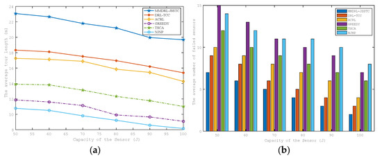
Figure 7. Impact of sensor energy capacity on the (a) average tour length (b) average number of failed sensors.

In addition, it can be found from Table 4 that the fixed charging upper threshold of the approaches based on the reinforcement learning framework is smaller than that of other heuristic approaches. Hence, the moving distance of the DRL-TCC and ACRL is slightly longer than that of the heuristic approaches, while they have fewer failed sensors. The proposed approach always has the least number of failed sensors during the test, thanks to the fact that MC can adaptively adjust the charging upper threshold according to the real-time charging demand and leave the current sensor in advance to charge the sensor with more urgent charging demand. However, the average tour length of the proposed approach is much longer than other approaches, which not only involves moving between sensors but also requires the MC to return to the charging service station more frequently to change the battery.

6.2. Impact of MC Energy Capacity on Charging Performance

The impact of MC energy capacity on the average tour length and the average number of failed sensors are shown in Figure 8a,b. They have similar trends to those in Figure 7a,b. This is because, as the energy capacity of the MC increases, MC has more operating space to perform charging actions, and more sensors with urgent charging demand can be charged in time to avoid failure in advance. Furthermore, MC can reduce the time to return to the charging service station to replace the battery, thereby effectively reducing the tour length.

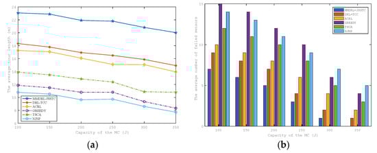
Figure 8. Impact of the MC energy capacity on the (a) average tour length (b) average number of failed sensors.

6.3. Impact of the Charging Speed on Charging Performance

We also analyze the impact of charging speed on charging performance. The test results are described in Figure 9a,b. As the charging speed increases, the average tour length of MC increases, and the average number of failed sensors decreases.

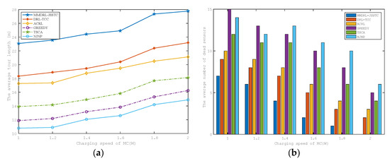
Figure 9. Impact of the MC charging speed on the (a) average tour length (b) average number of failed sensors.

This is because the increased charging speed can effectively reduce the time required for charging, and MC needs to return to the charging service station and move between sensors more frequently, so the moving distance increases. Due to the shorter charging time, the probability of charging sensors with urgent charging demand in time is greatly improved. Therefore, the average number of failed sensors decreases significantly.

6.4. Impact of the Moving Speed on Charging Performance

We evaluate the impact of MC moving speed on charging performance in this section, which is shown in Figure 10a,b. They have a trend similar to Figure 9a,b. This is because, with the increased charging speed, the time to move between the charging destinations is effectively shortened, allowing the MC to reach the sensors with more urgent charging demands faster.

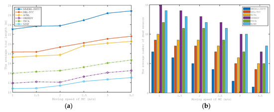
Figure 10. Impact of the MC moving speed on the (a) average tour length (b) average number of failed sensors.

6.5. Comparison of Network Lifetime

The above experiments discuss the impact of different parameter changes on charging performance based on the preset lifetime. This section compares the lifetime distribution of six mobile charging approaches based on different scenarios, including JSSTC50, JSSTC100, and JSSTC200. To compare the impact of different approaches to prolonging the lifetime, we also add the lifetime distribution of the network where the sensors are not charged. In particular, each approach has been run 50 times, and the results are shown in Figure 11.

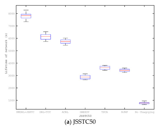
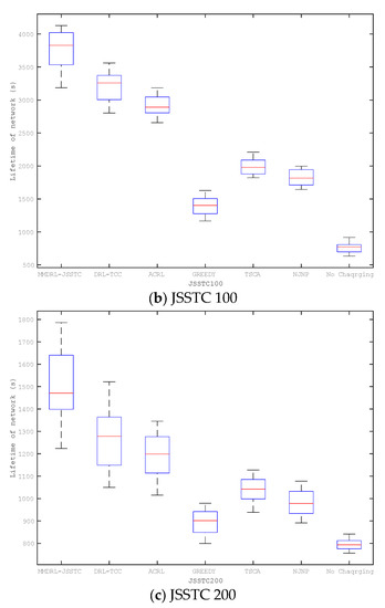
Figure 11. Comparison of network lifetime (a) JSSTC50, (b) JSSTC 100, and (c) JSSTC 200.

Obviously, the approaches based on reinforcement learning framework can obtain longer lifetime than those heuristic approaches. Among the heuristic approaches, the lifetime of the greedy approach is always the shortest. The lifetime of the proposed approach is always the longest in different scenarios, and it becomes more outstanding as the number of sensors increases. This is because the proposed approach can adaptively adjust the charging upper threshold of the sensor. Furthermore, introducing Bi-GRU can also train the agent based on the historical and future state information to determine charging actions that prolong the network lifetime.

7. Conclusions and Future Work

This paper studies a novel joint mobile charging sequence scheduling and charging upper threshold control problem (JSSTC), which can adaptively adjust the charging upper threshold of the sensor. A novel multi-discrete action space deep Q-network approach is proposed for JSSTC (MDDRL-JSSTC), where the MC is employed as an agent to explore the environment. The agent gives a two-dimensional action at each time step, including the charging destination and the corresponding charging upper threshold. The bidirectional gated recurrent unit is introduced in the Q-network to guide the agent in acquiring better charging decisions based on historical and future state information. Simulation results show that the proposed approach can significantly prolong the network lifetime and reduce the number of failed sensors.

As future work, the construction of a suitable test platform and the design of multiple MC collaborative mobile charging scheduling schemes will be our focus.

References

- Kaswan, A.; Jana, P.K.; Das, S.K. A Survey on Mobile Charging Techniques in Wireless Rechargeable Sensor Networks. IEEE Commun. Surv. Tutor. 2022, 24, 1750–1779. [Google Scholar] [CrossRef]
- Kuila, P.; Jana, P.K. Energy Efficient Clustering and Routing Algorithms for Wireless Sensor Networks: Particle Swarm Optimization Approach. Eng. Appl. Artif. Intell. 2014, 33, 127–140. [Google Scholar] [CrossRef]
- Zhang, C.; Zhou, G.; Li, H.; Cao, Y. Manufacturing Blockchain of Things for the Configuration of a Data-and Knowledge-Driven Digital Twin Manufacturing Cell. IEEE Internet Things J. 2020, 7, 11884–11894. [Google Scholar] [CrossRef]
- Wang, Y.; Rajib, S.M.S.M.; Collins, C.; Grieve, B. Low-Cost Turbidity Sensor for Low-Power Wireless Monitoring of Fresh-Water Courses. IEEE Sens. J. 2018, 18, 4689–4696. [Google Scholar] [CrossRef]
- Shi, Y.; Xie, L.; Hou, Y.T.; Sherali, H.D. On Renewable Sensor Networks with Wireless Energy Transfer. In Proceedings of the 2011 Proceedings IEEE INFOCOM, Shanghai, China, 10–15 April 2011; pp. 1350–1358. [Google Scholar] [CrossRef]
- Wang, C.; Li, J.; Ye, F.; Yang, Y. A Mobile Data Gathering Framework for Wireless Rechargeable Sensor Networks with Vehicle Movement Costs and Capacity Constraints. IEEE Trans. Comput. 2016, 65, 2411–2427. [Google Scholar] [CrossRef]
- Li, J.; Jiang, C.; Wang, J.; Xu, T.; Xiao, W. Mobile Charging Sequence Scheduling for Optimal Sensing Coverage in Wireless Rechargeable Sensor Networks. Appl. Sci. 2023, 13, 2840. [Google Scholar] [CrossRef]
- Lin, C.; Wu, Y.; Liu, Z.; Obaidat, M.S.; Yu, C.W.; Wu, G. GTCharge: A Game Theoretical Collaborative Charging Scheme for Wireless Rechargeable Sensor Networks. J. Syst. Softw. 2016, 121, 88–104. [Google Scholar] [CrossRef]
- He, L.; Kong, L.; Gu, Y.; Pan, J.; Zhu, T. Evaluating the On-Demand Mobile Charging in Wireless Sensor Networks. IEEE Trans. Mob. Comput. 2015, 14, 1861–1875. [Google Scholar] [CrossRef]
- Lin, C.; Zhou, J.; Guo, C.; Song, H.; Wu, G.; Obaidat, M.S. TSCA: A Temporal-Spatial Real-Time Charging Scheduling Algorithm for On-Demand Architecture in Wireless Rechargeable Sensor Networks. IEEE Trans. Mob. Comput. 2018, 17, 211–224. [Google Scholar] [CrossRef]
- Tomar, A.; Muduli, L.; Jana, P.K. A Fuzzy Logic-Based On-Demand Charging Algorithm for Wireless Rechargeable Sensor Networks with Multiple Chargers. IEEE Trans. Mob. Comput. 2021, 20, 2715–2727. [Google Scholar] [CrossRef]
- Cao, X.; Xu, W.; Liu, X.; Peng, J.; Liu, T. A Deep Reinforcement Learning-Based on-Demand Charging Algorithm for Wireless Rechargeable Sensor Networks. Ad Hoc Netw. 2021, 110, 102278. [Google Scholar] [CrossRef]
- Yang, M.; Liu, N.; Zuo, L.; Feng, Y.; Liu, M.; Gong, H.; Liu, M. Dynamic Charging Scheme Problem with Actor–Critic Reinforcement Learning. IEEE Internet Things J. 2021, 8, 370–380. [Google Scholar] [CrossRef]
- Bui, N.; Nguyen, P.L.; Nguyen, V.A.; Do, P.T. A Deep Reinforcement Learning-Based Adaptive Charging Policy for Wireless Rechargeable Sensor Networks. arXiv 2022. [Google Scholar] [CrossRef]
- Tang, L.; Chen, Z.; Cai, J.; Guo, H.; Wu, R.; Guo, J. Adaptive Energy Balanced Routing Strategy for Wireless Rechargeable Sensor Networks. Appl. Sci. 2019, 9, 2133. [Google Scholar] [CrossRef]
- Jiang, C.; Wang, Z.; Chen, S.; Li, J.; Wang, H.; Xiang, J.; Xiao, W. Attention-Shared Multi-Agent Actor–Critic-Based Deep Reinforcement Learning Approach for Mobile Charging Dynamic Scheduling in Wireless Rechargeable Sensor Networks. Entropy 2022, 24, 965. [Google Scholar] [CrossRef]
- Shu, Y.; Shin, K.G.; Chen, J.; Sun, Y. Joint Energy Replenishment and Operation Scheduling in Wireless Rechargeable Sensor Networks. IEEE Trans. Ind. Inform. 2017, 13, 125–134. [Google Scholar] [CrossRef]
- Malebary, S. Wireless Mobile Charger Excursion Optimization Algorithm in Wireless Rechargeable Sensor Networks. IEEE Sens. J. 2020, 20, 13842–13848. [Google Scholar] [CrossRef]
- Zhong, P.; Xu, A.; Zhang, S.; Zhang, Y.; Chen, Y. EMPC: Energy-Minimization Path Construction for Data Collection and Wireless Charging in WRSN. Pervasive Mob. Comput. 2021, 73, 101401. [Google Scholar] [CrossRef]
- Kingma, D.P.; Ba, J. Adam: A Method for Stochastic Optimization. arXiv 2017. [Google Scholar] [CrossRef]
Disclaimer/Publisher’s Note: The statements, opinions and data contained in all publications are solely those of the individual author(s) and contributor(s) and not of MDPI and/or the editor(s). MDPI and/or the editor(s) disclaim responsibility for any injury to people or property resulting from any ideas, methods, instructions or products referred to in the content. |
© 2023 by the authors. Licensee MDPI, Basel, Switzerland. This article is an open access article distributed under the terms and conditions of the Creative Commons Attribution (CC BY) license (https://creativecommons.org/licenses/by/4.0/).