
New Correlations for the Determination of Undrained Shear, Elastic Modulus, and Bulk Density Based on Dilatometer Tests (DMT) for Organic Soils in the South of Quito, Ecuador


Abstract
:1. Introduction
2. Overview
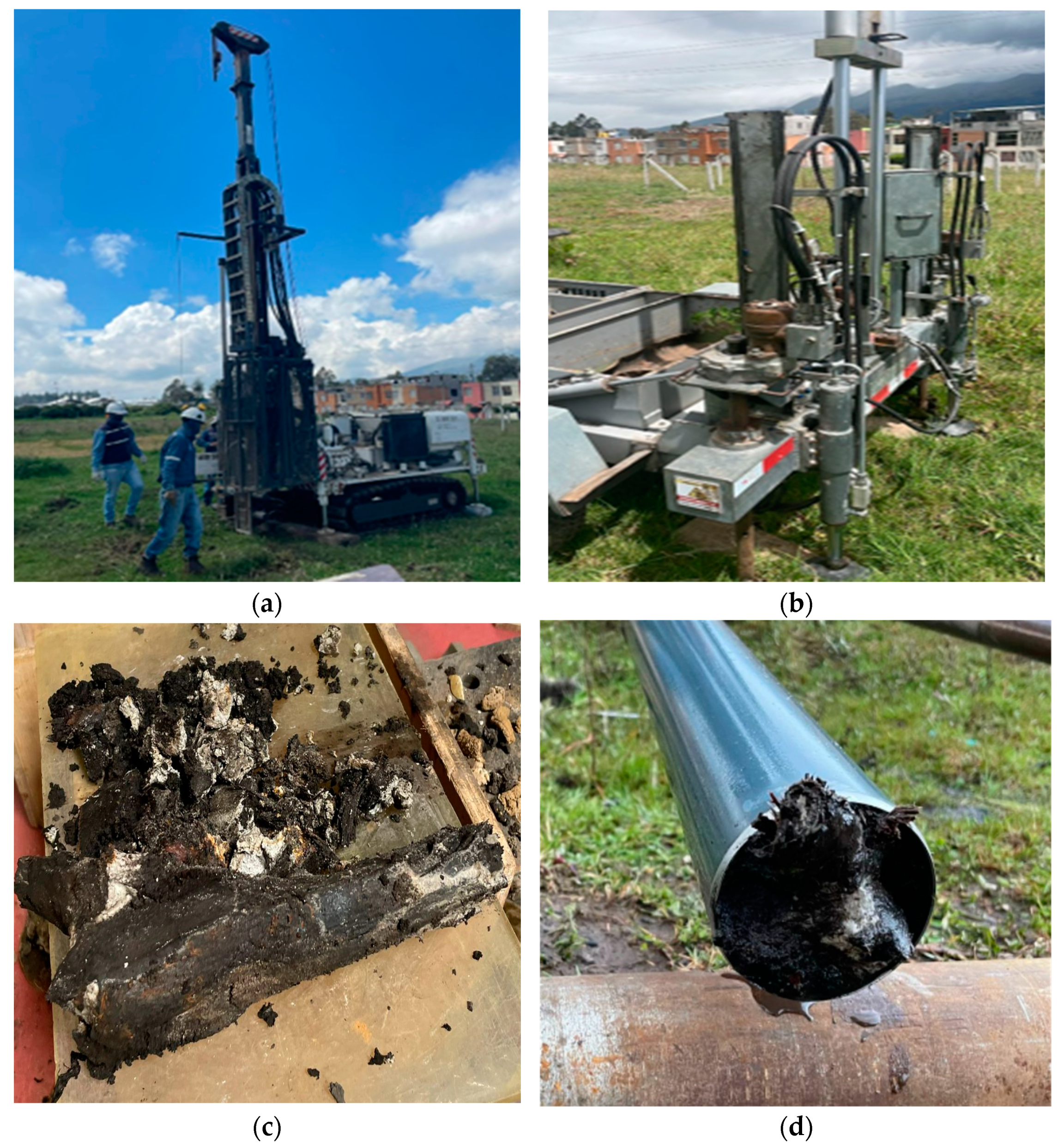
2.1. Test Site
2.2. Laboratory Tests
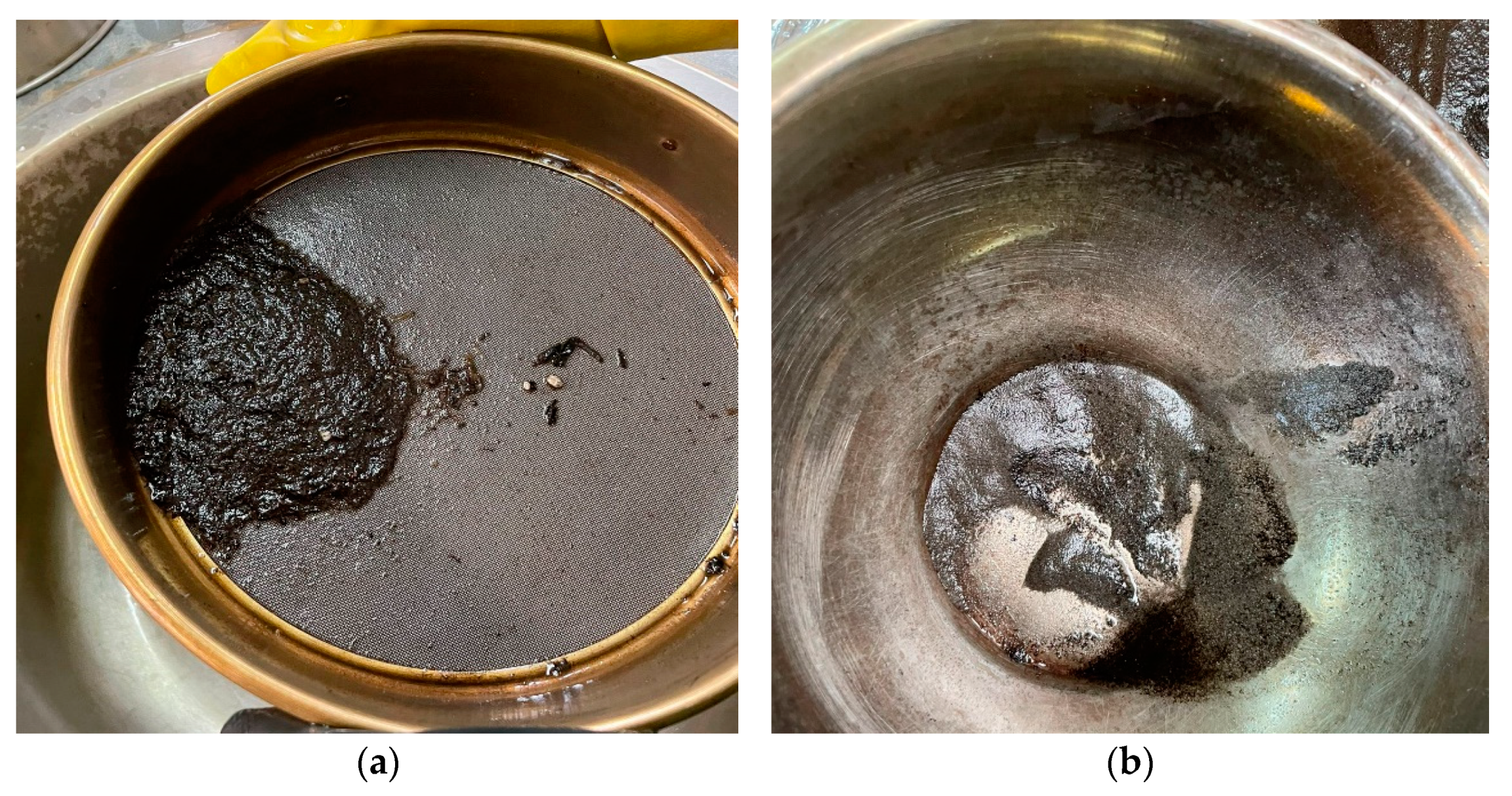
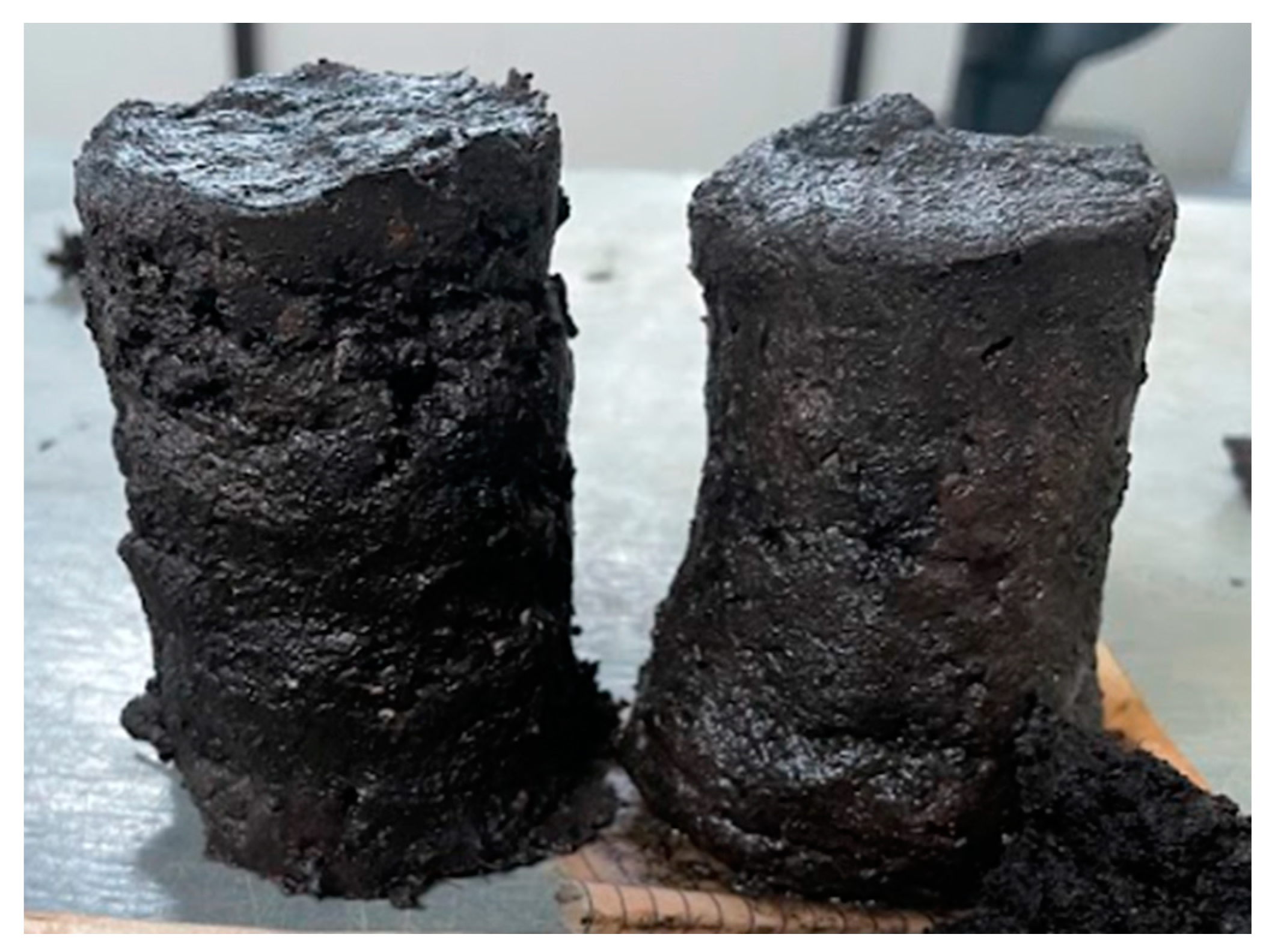
Specimen Preparation
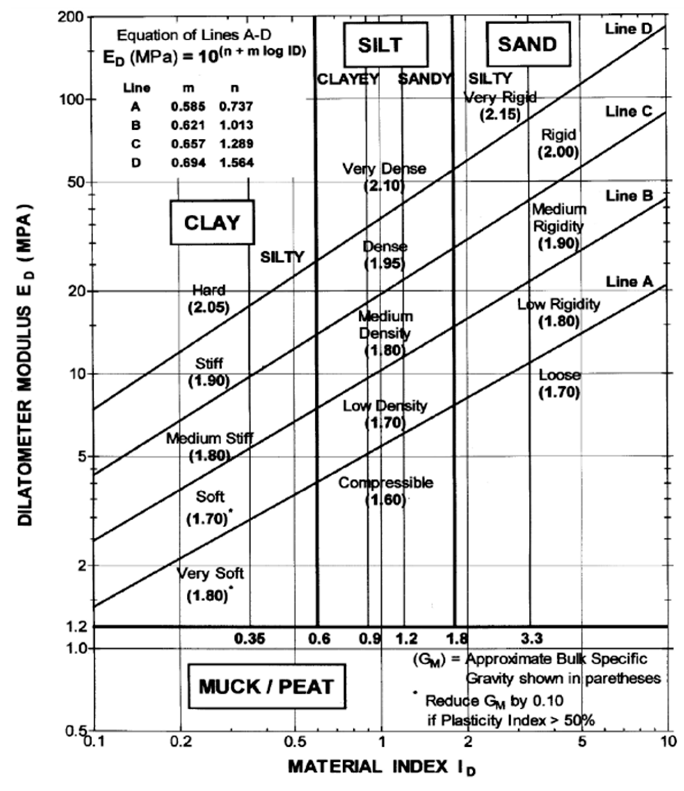
2.3. Marchetti Dilatometer: Conceptualization
3. Results
3.1. Laboratory Tests Results
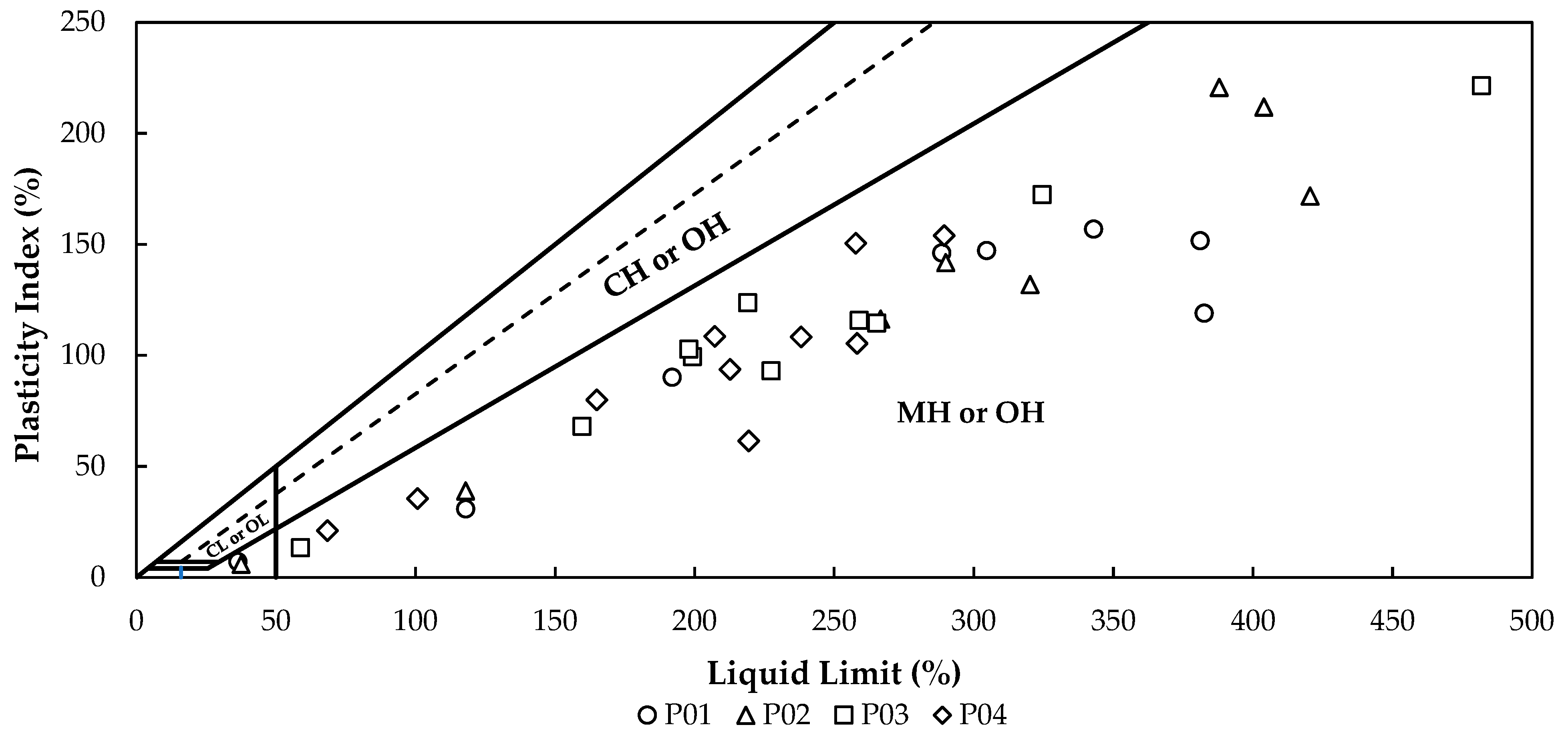
3.1.1. Atterberg Limits
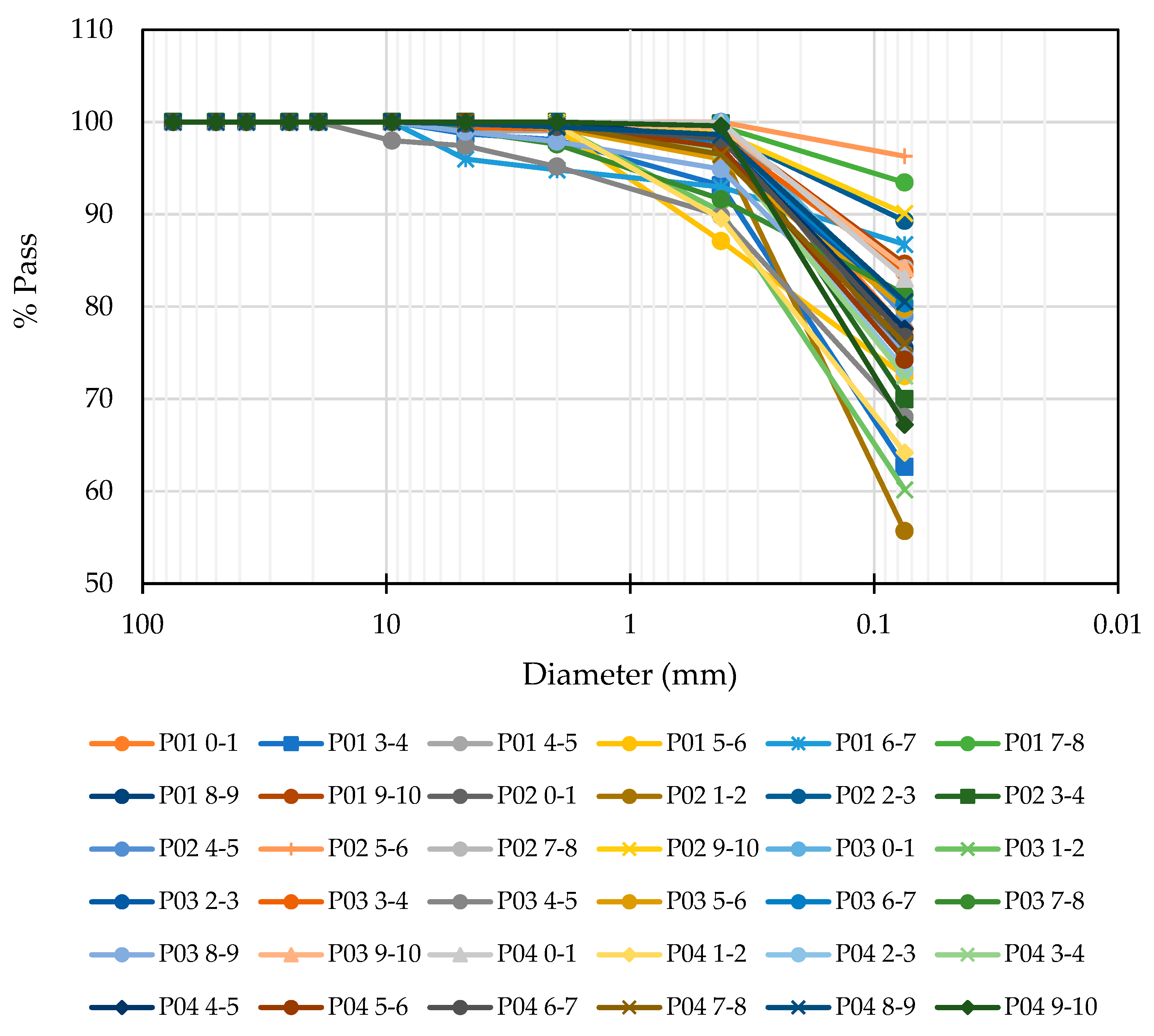
3.1.2. Granulometry
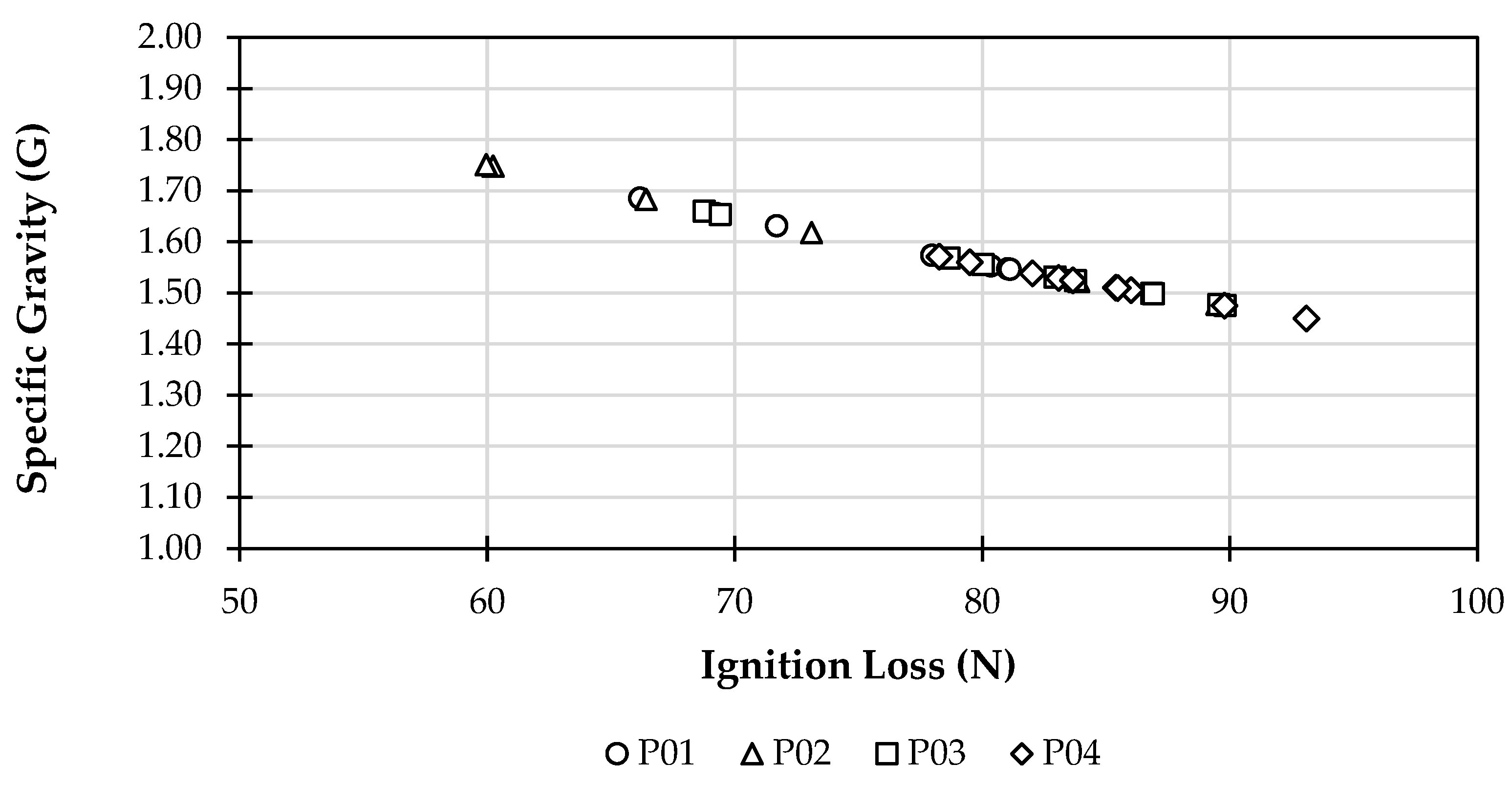
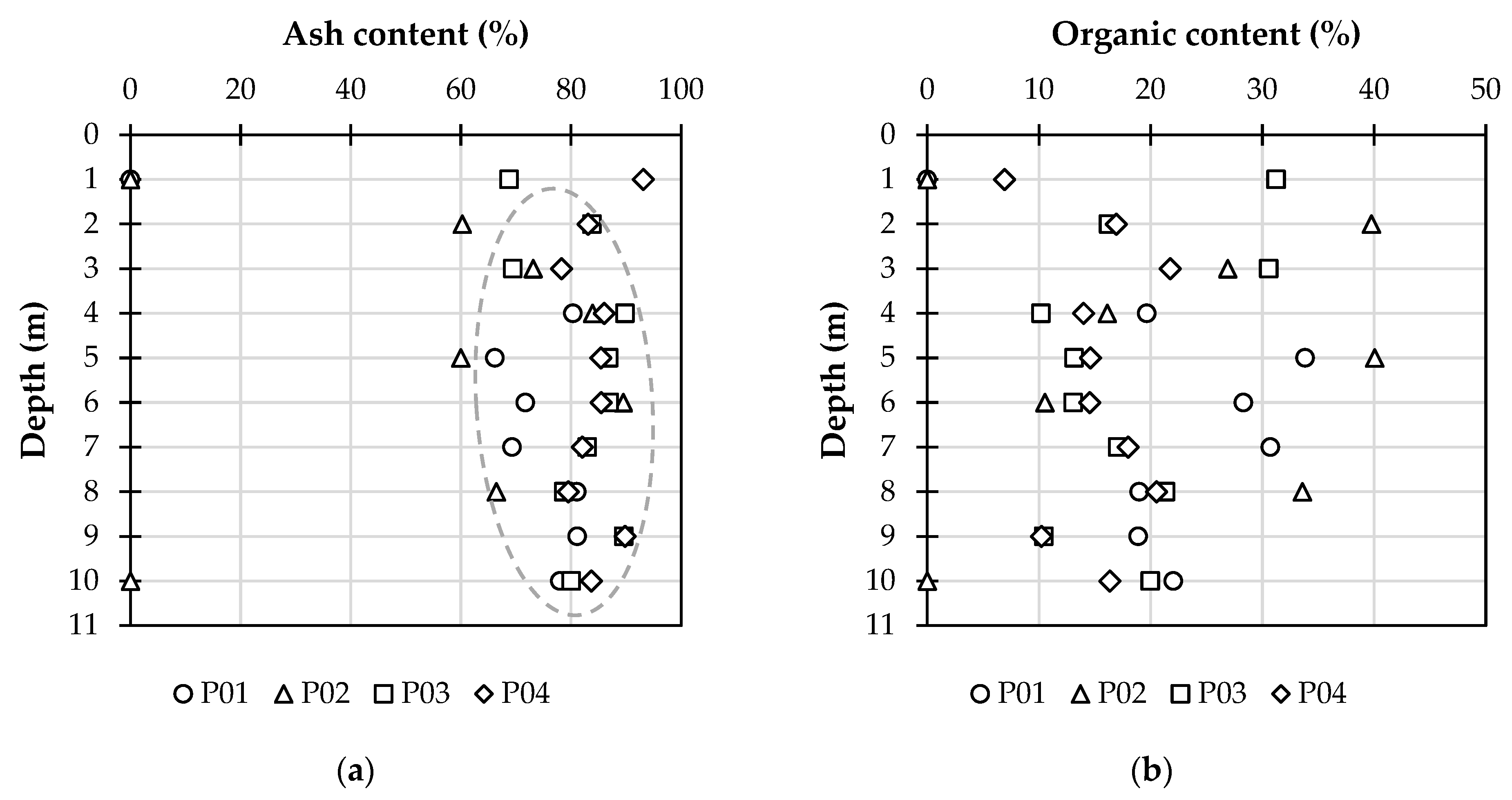
3.1.3. Ash and Organic Content
3.1.4. Summary of Laboratory Tests Results
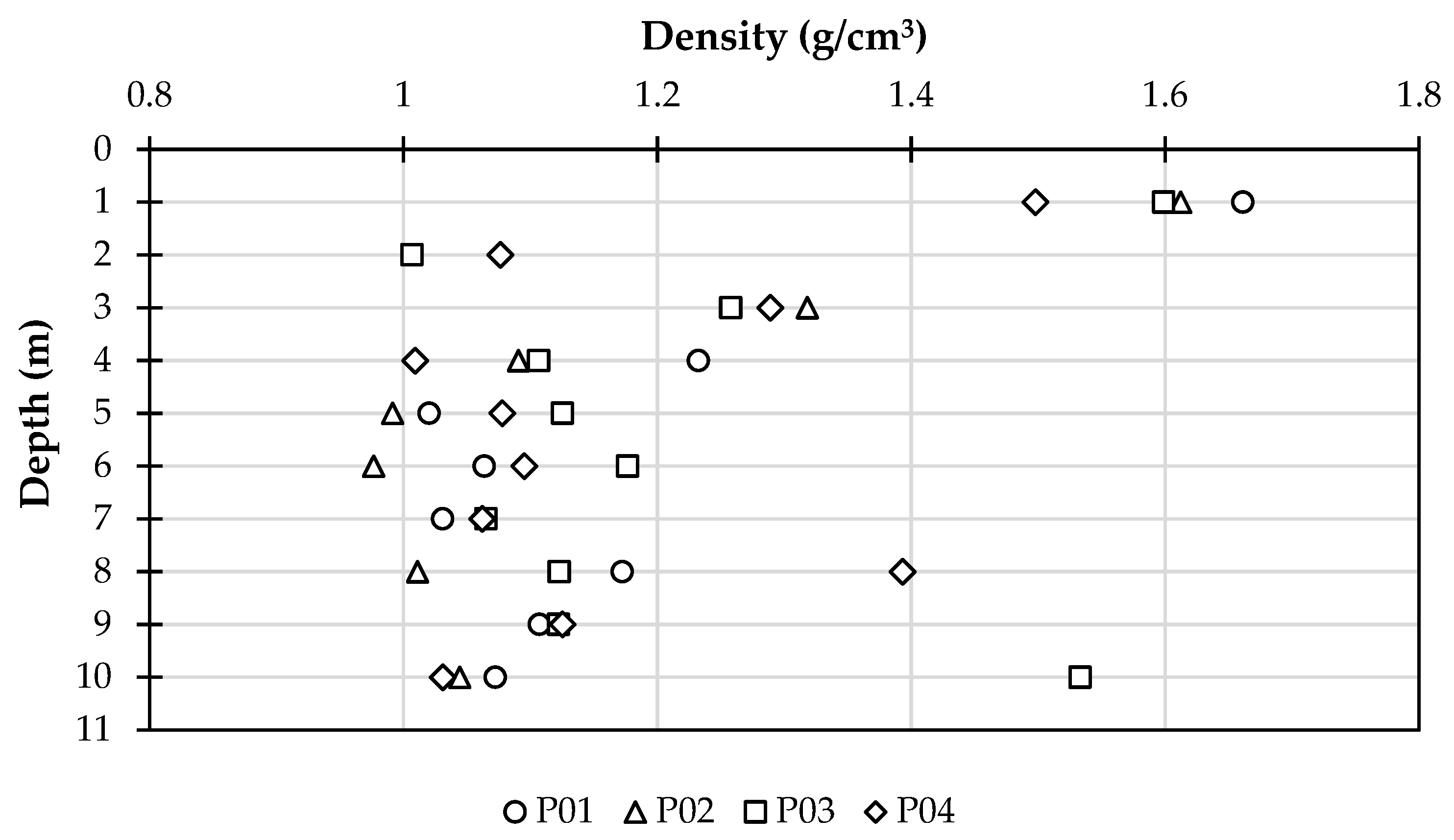
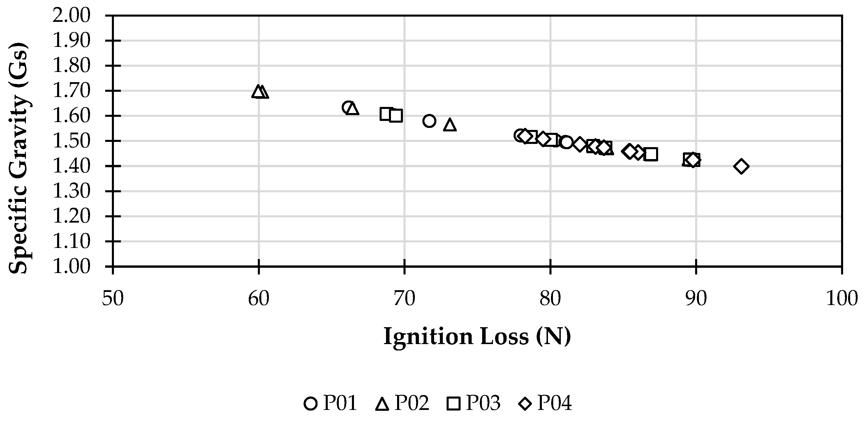
3.1.5. Density (Unit Weight) of Soil
3.1.6. Relative Density
3.1.7. Triaxial UU
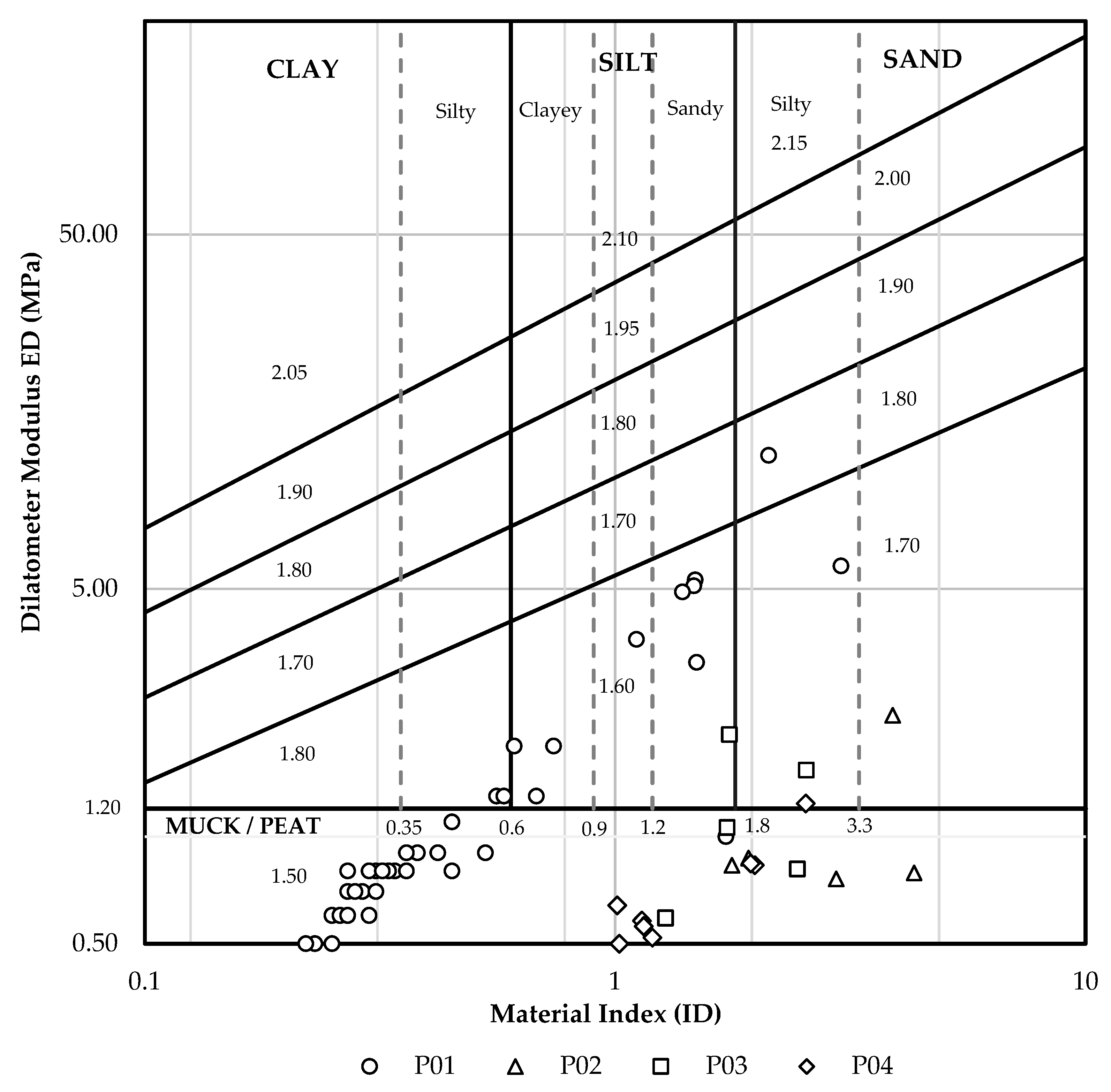
3.2. Dilatometer Results
4. Discussion
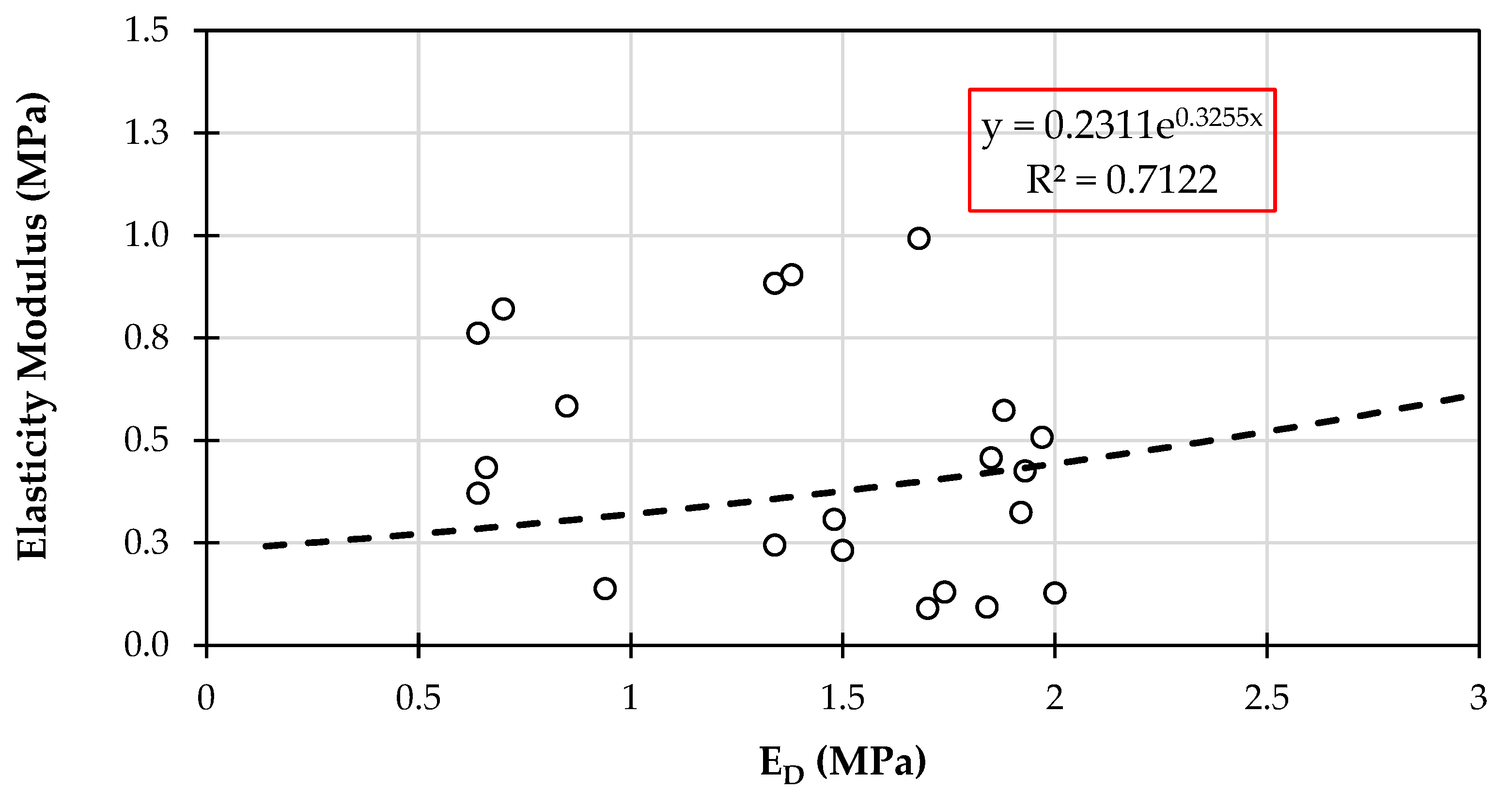
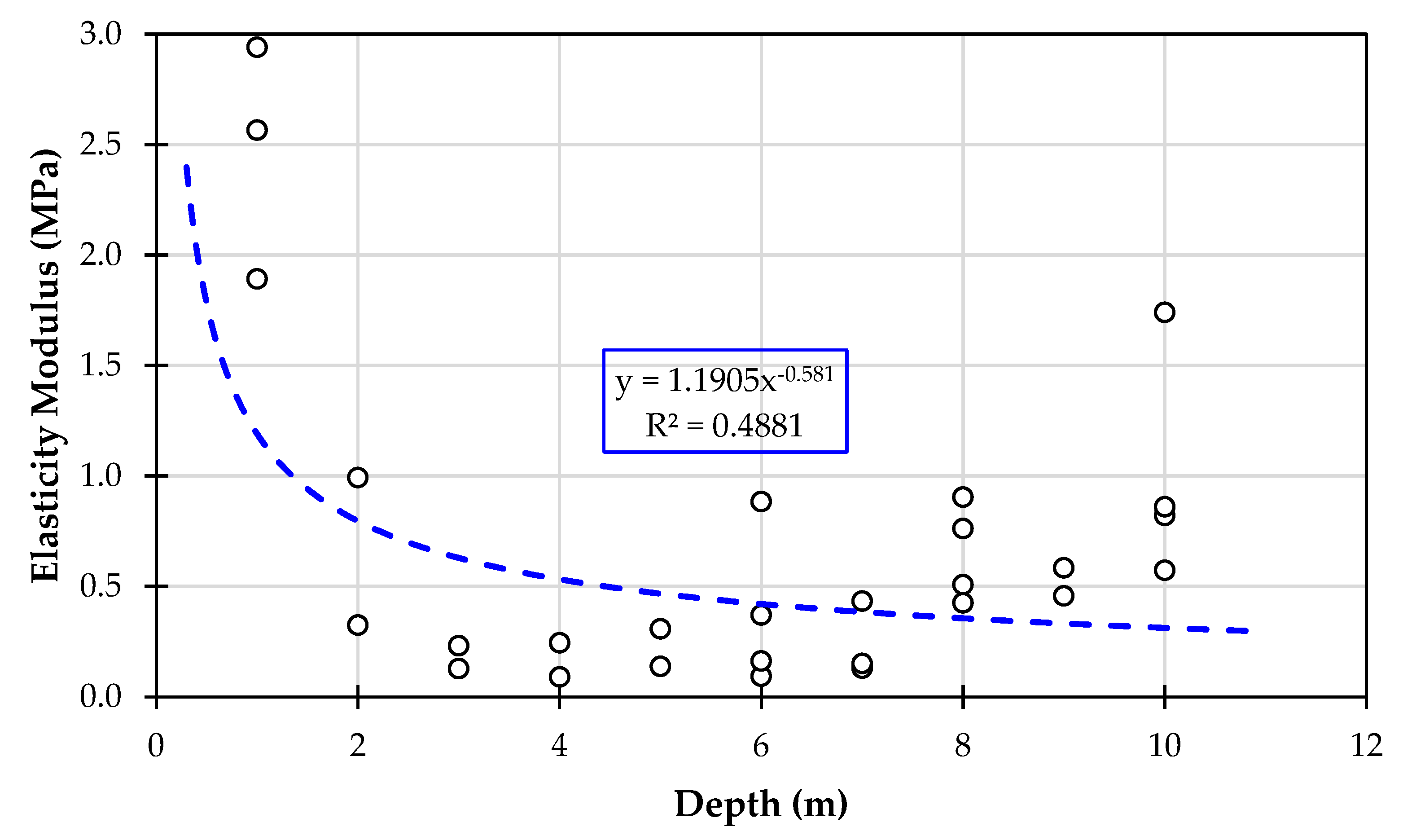
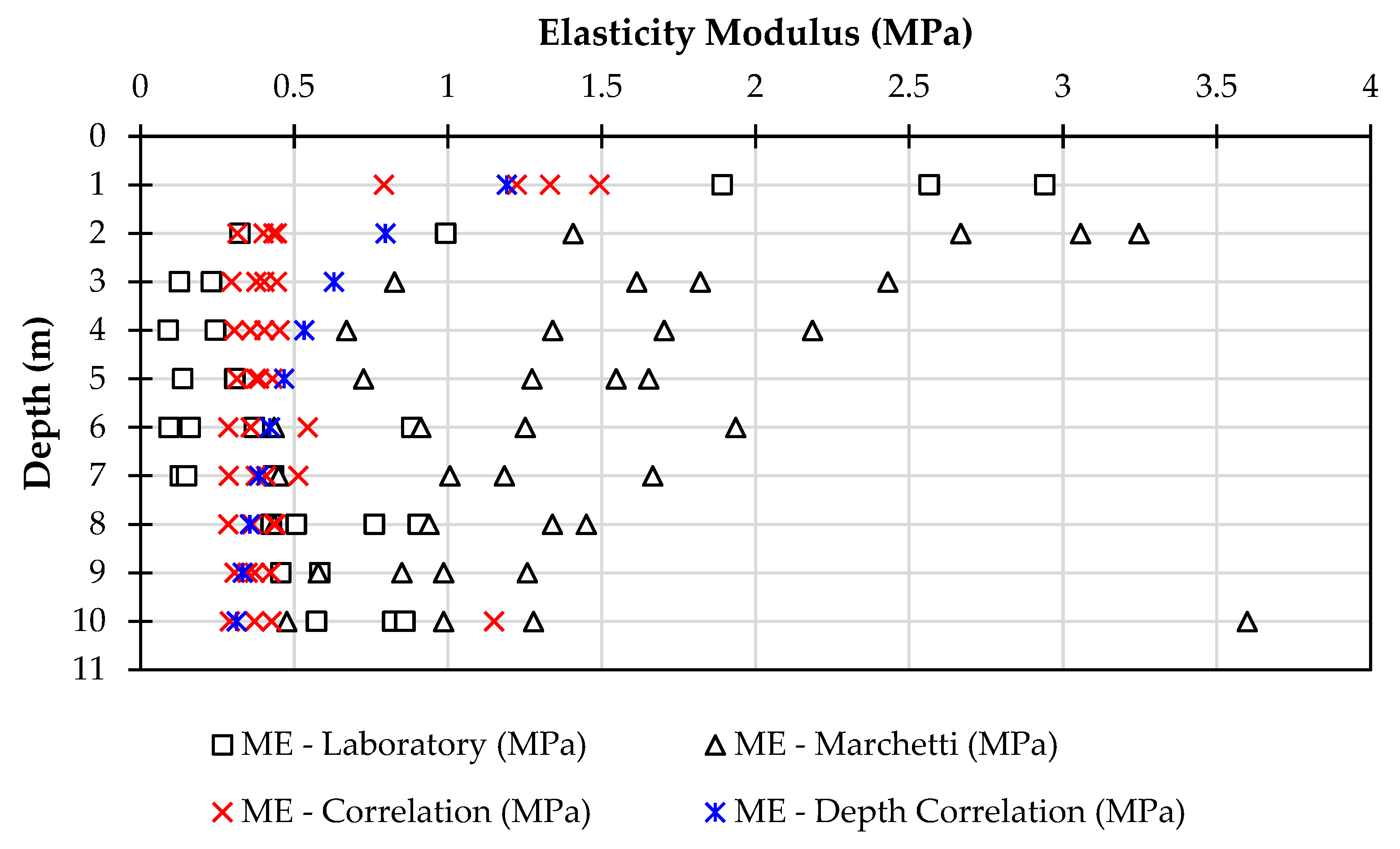
4.1. Elasticity Modulus (E)
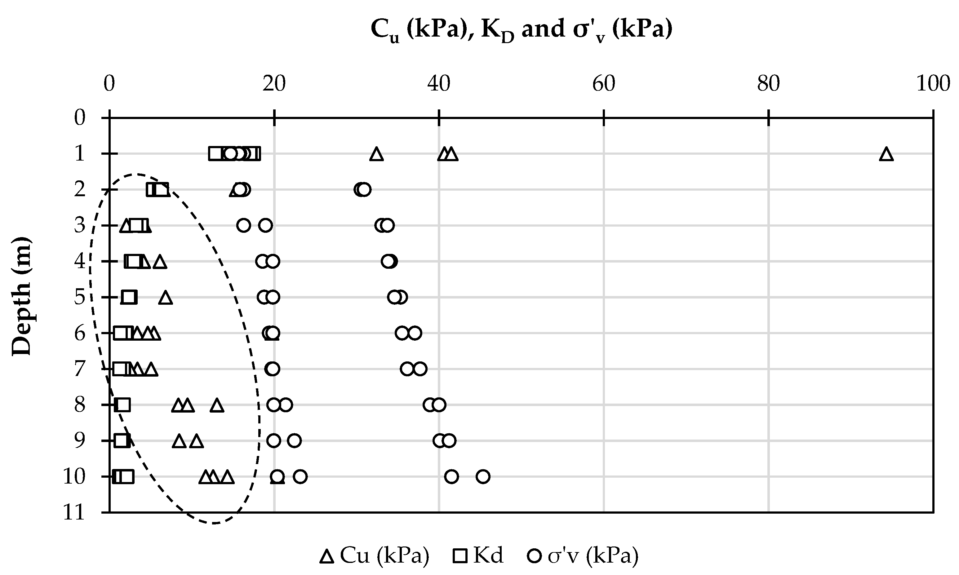
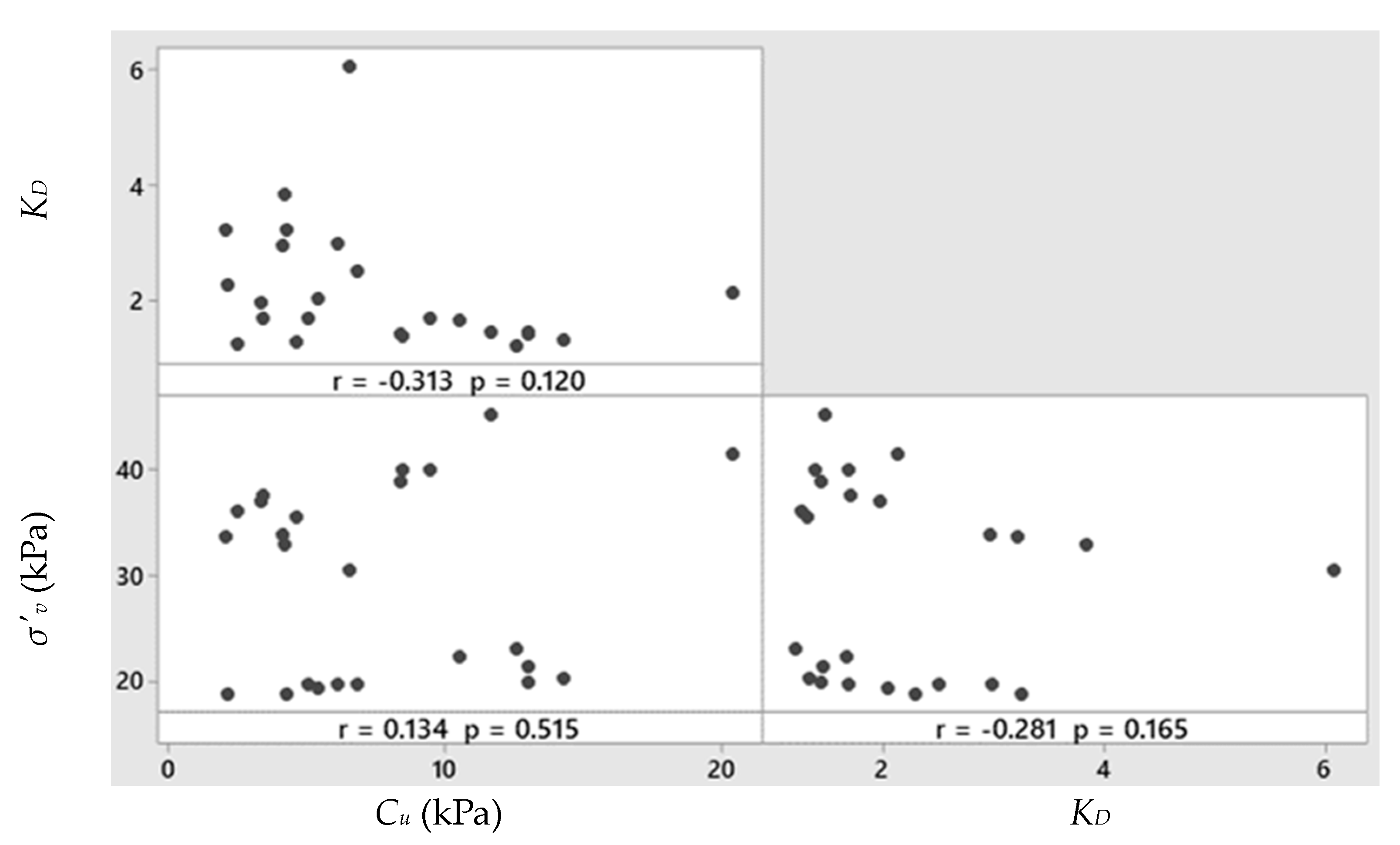
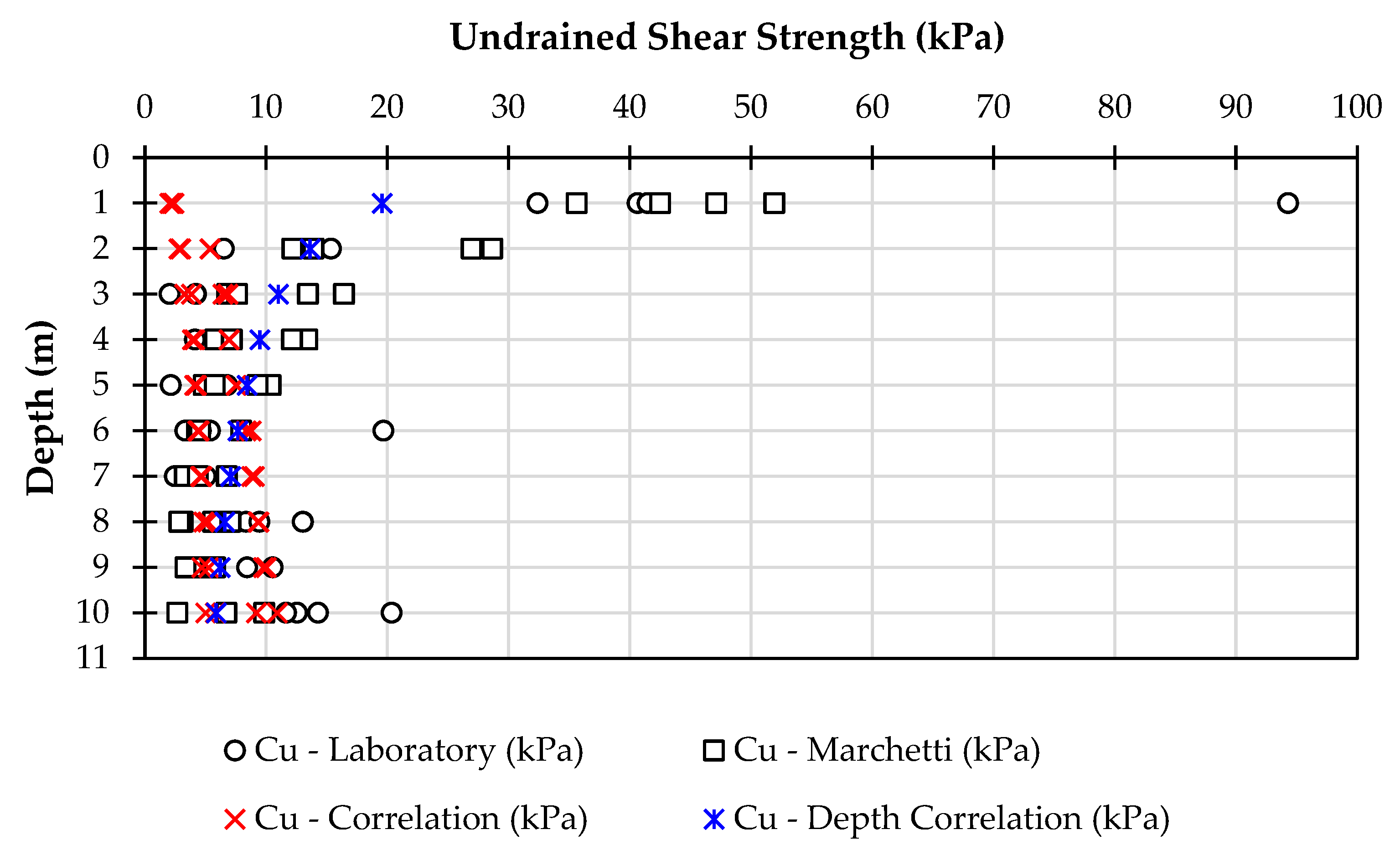
4.2. Undrained Shear Strength (Cu)
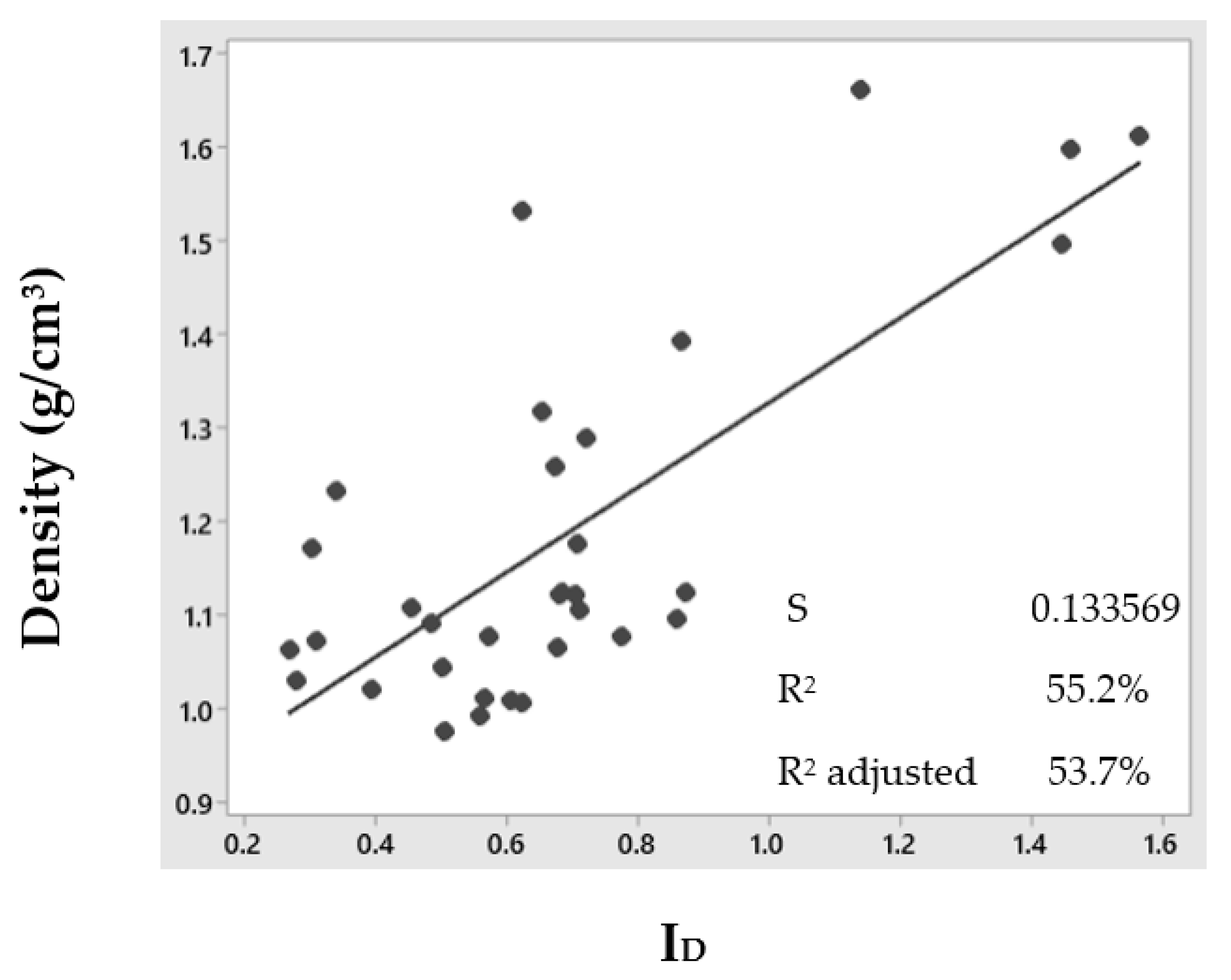
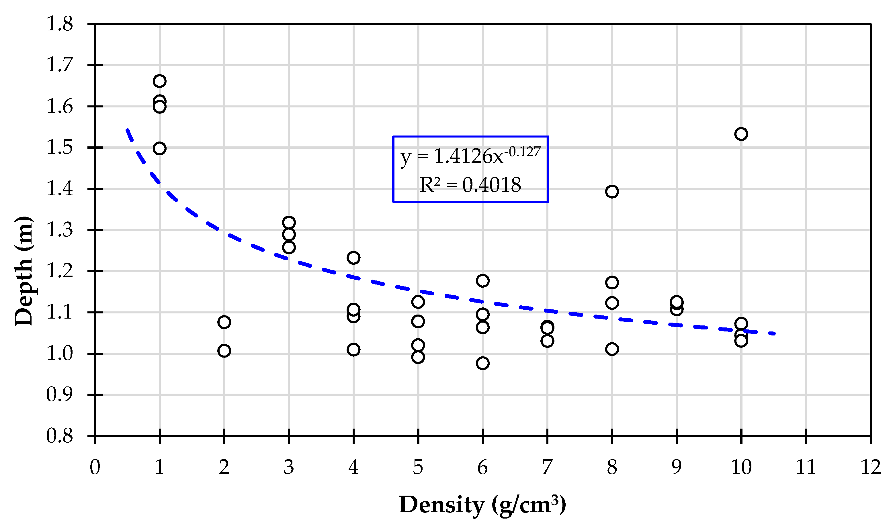
4.3. Density
4.4. Final Equations
5. Conclusions
Author Contributions
Funding
Institutional Review Board Statement
Informed Consent Statement
Data Availability Statement
Acknowledgments
Conflicts of Interest
References
- Marchetti, S.; Marchetti, D.; Villalobos, F. El Dilatómetro Sísmico SDMT para ensayos de suelos in situ. Obras Y Proy. 2013, 20–29. [Google Scholar] [CrossRef] [Green Version]
- Marchetti, S.; Monaco, P.; Tonati, G.; Clabrese, M. The Flat Dilatometer Test (DMT) in Soil Investigations; International Society for Soil Mechanics and Geotechnical Engineering (ISSMGE): London, UK, 2001. [Google Scholar]
- Sánchez, J.D.A. Determination of the undrained shear strength of organic soils using the Cone Penetration Test and Marchetti’s Flat Dilatometer Test. Puce 2018, 106, 3–39. [Google Scholar]
- Rabarijoely, S. A New Approach to the Determination of Mineral and Organic Soil Types Based on Dilatometer Tests (DMT). Appl. Sci. 2018, 8, 2249. [Google Scholar] [CrossRef] [Green Version]
- Bandyopadhyay, K.; Das, K.; Nandi, S.; Halder, A. Dilatometer-an in Situ Soil Exploration Tool for Problematic Ground Conditions vis-à-vis for Economizing Construction Activities. Indian Geotech. J. 2022, 52, 1155–1170. [Google Scholar] [CrossRef]
- Marchetti, S. Some 2015 Updates to the TC16 DMT Report 2001. In Proceedings of the 3rd International Conference on the Flat Dilatometer, Roma, Italy, 14–16 June 2015; Available online: www.marchetti-dmt.it (accessed on 11 July 2023).
- Burlon, S.; Frikha, W.; Monaco, P. Session report: Pressuremeter and Dilatometer. In Proceedings of the 5th Geotechnical and Geophysical Site Characterization ISC’5, Sydney, Australia, 5–9 September 2016; pp. 259–269. [Google Scholar]
- Amoroso, S.; Monaco, P.; Minarelli, L.; Stefani, M.; Marchetti, D. Estimation of geotechnical parameters by CPTu and DMT data: A case study in Emilia Romagna (Italy). In Cone Penetration Testing 2018, Proceedings of the 4th International Symposium on Cone Penetration Testing (CPT’18), 21–22 June 2018, Delft, The Netherlands; Hicks, M.A., Pisanò, F., Peuchen, J., Eds.; CRC Press: Boca Raton, FL, USA, 2018; pp. 85–91. [Google Scholar]
- Monnet, J. Tests by Flat Dilatometer (DMT). In In Situ Tests in Geotechnical Engineering; John Wiley & Sons, Ltd.: Hoboken, NJ, USA, 2015; pp. 105–112. [Google Scholar] [CrossRef]
- Shen, H.; Haegeman, W.; Peiffer, H. Instrumented DMT: Review and Analysis. In Proceedings of the 3rd International Conference on the Flat Dilatometer, Rome, Italy, 14–16 June 2015. [Google Scholar]
- Berisavljevic, D.M.; Berisavljevic, Z.M. Dilatometer and seismic dilatometer tests in different depositional environments. In Proceedings of the 6th International Conference on Geotechnical and Geophysical Site Characterization (ISC2020), Budapest, Hungary, 7–11 September 2020. [Google Scholar]
- Liu, X.-Y.; Zhu, D.; Yuan, D. Improvement and application of flat dilatometer. Chin. J. Geotech. Eng. 2013, 35, 1375–1380. [Google Scholar]
- Benoı⁁t, J.; Stetson, K.P. Use of an Instrumented Flat Dilatometer in Soft Varved Clay. J. Geotech. Geoenvironmental Eng. 2003, 129, 1159–1167. [Google Scholar] [CrossRef]
- Santander Vásquez, P.E. Informe Técnico de Inspección Provincia de Pichincha-Quito Sector Turubamba; Secretaría Nacional de Gestión de Riesgos: Quito, Ecuador, 2013. [Google Scholar]
- ASTM D1587-15; Standard Practice for Thin-Walled Tube Sampling of Fine-Grained Soils for Geotechnical Purposes 1. ASTM International: West Conshohocken, PA, USA, 2015. [CrossRef]
- ASTM D2216-19; Standard Test Method for Laboratory Determination of Water (Moisture) Content of Soil and Rock by Mass. ASTM International: West Conshohocken, PA, USA, 2019; pp. 1–5. [CrossRef]
- ASTM D4318-17; Standard Test Methods for Liquid Limit, Plastic Limit, and Plasticity Index of Soils. ASTM International: West Conshohocken, PA, USA, 2017; Volume 4, pp. 1–14. [CrossRef]
- ASTM D1140-17; Standard Test Methods for Determining the Amount of Material Finer than 75-µm (No. 200) Sieve in Soils by Washing. ASTM International: West Conshohocken, PA, USA, 2017; pp. 1–6.
- ASTM D2487-17; Standard Practice for Classification of Soils for Engineering Purposes (Unified Soil Classification System) D2487-00. ASTM International: West Conshohocken, PA, USA, 2017; Volume 4, pp. 249–260.
- ASTM D2974; Standard Test Methods for Determining the Water (Moisture) Content, Ash Content, and Organic Material of Peat and Other Organic Soils. ASTM International: West Conshohocken, PA, USA, 2020; pp. 1–4.
- ASTM D7263-21; Standard Test Methods for Laboratory Determination of Density (Unit Weight) of Soil. ASTM International: West Conshohocken, PA, USA, 2021; Volume i, pp. 1–7.
- ASTM D2850-15; Standard Test Method for Unconsolidated-Undrained Triaxial Compression Test on Cohesive Soils. ASTM International: West Conshohocken, PA, USA, 2015; Volume D2850−15, pp. 1–6.
- Marchetti, S. In Situ Tests by Flat Dilatometer. J. Geotech. Eng. Div. 1980, 106, 299–321. [Google Scholar] [CrossRef]
- ASTM D6635-15; Standard Test Method for Performing the Flat Plate Dilatometer 1. ASTM International: West Conshohocken, PA, USA, 2016. [CrossRef]
- Larsson, R. Dilatometerförsök. En In-Situ Metod för Bestämning av Lagerföljd Och Egenskaper i Jord. Dilatometer Test. An In-Situ Method for the Determination of Layer Sequences and Soil Properties; Statens Geotekniska Institut: Linköping, Sweden, 1993. [Google Scholar]
- Rabarijoely, S. New chart for classification of organic soils from dilatometer tests (DMT) results. Ann. Warsaw Univ. Life Sci. SGGW 2013, 2, 159–168. [Google Scholar] [CrossRef]
- Cruz, N.; Cruz, J.; Rodrigues, C.; Cruz, M.; Amoroso, S. Behaviour of granitic residual soils assessed by SCPTu and other in-situ tests. In Cone Penetration Testing 2018, Proceedings of the 4th International Symposium on Cone Penetration Testing, CPT 2018, Delft, The Netherlands, 21–22 June 2018; Delft Univ Technol: Delft, The Netherlands, 2018; pp. 241–247. [Google Scholar]
- Das, K.; Nandi, S.; Chattaraj, S.; Halder, A.; Sadhukhan, W. Estimation of subsoil parameters and settlement of foundation for a project in Kolkata based on CPT, DMT. J. Phys. Conf. Ser. 2022, 2286, 012026. [Google Scholar] [CrossRef]
- Sutejo, Y.; Saggaff, A.; Rahayu, W.; Hanafiah. Physical and chemical characteristics of fibrous peat. AIP Conf. Proc. 2017, 1903, 090006. [Google Scholar] [CrossRef] [Green Version]
- ASTM D653-22; Standard Terminology Relating to Soil, Rock, and Contained Fluids. ASTM International: West Conshohocken, PA, USA, 2022. [CrossRef]
- Rabarijoely, S.; Lech, M.; Bajda, M. Determination of relative density and degree of saturation in mineral soils based on in situ tests. Materials 2021, 14, 6963. [Google Scholar] [CrossRef]
- Skempton, A.W.; Petley, D.J. Ignition Loss and other Properties of Peats and Clays from Avonmouth, King’s Lynn and Cranberry Moss. Geotechnique 1970, 20, 343–356. [Google Scholar] [CrossRef]
- Li, W.; O’Kelly, B.C.; Yang, M.; Fang, K.; Li, X.; Li, H. Briefing: Specific gravity of solids relationship with ignition loss for peaty soils. Geotech. Res. 2020, 7, 134–145. [Google Scholar] [CrossRef]
- Head, K.H.; Epps, R.J. Manual of Soil Laboratory Testing. Volume 3, Effective Stress Tests; Whittles Publishing: Caithness, UK, 2014. [Google Scholar]
- Briaud, J.L.; Spencer, J. Introduction to Soil Moduli. Eotechnical News 2001, 19, 54–58. [Google Scholar]
- Akpila, B.; Omunguye, I. Soil Modulus and Undrained Cohesion of Clayey Soils from Stress-Strain Models. Can. J. Pure Appl. Sci. 2014, 8, 3155–3161. [Google Scholar]
- Hernández Sampieri, R.; Fernández Collado, C.; Baptista Lucio, P. Metodología de la Investigación; McGraw Hill: New York, NY, USA, 2014. [Google Scholar]
- Wierzbicki, J. Evaluation of deformation parameters of organic subsoil by means of CPTU, DMT, SDMT. Archit. Civ. Eng. Environ. 2013, 4, 53–60. [Google Scholar]
- Lechowicz, Z.; Fukue, M.; Rabarijoely, S.; Sulewska, M.J. Evaluation of the undrained shear strength of organic soils from a dilatometer test using artificial neural networks. Appl. Sci. 2018, 8, 1395. [Google Scholar] [CrossRef] [Green Version]
- Konkol, J.; Międlarz, K.; Bałachowski, L. Geotechnical characterization of soft soil deposits in Northern Poland. Eng. Geol. 2019, 259, 105187. [Google Scholar] [CrossRef]


| Laboratory Test | Parameter | Number of Tests | Ref. |
|---|---|---|---|
| Moisture content | W (%) | 36 | [16] |
| Atterberg Limits | LL, LP, IP (%) | 36 | [17] |
| Material finer than 75 μm | %Fines | 36 | [18] |
| USCS Classification | Soil Classification | 36 | [19] |
| Ash and organic content | Ash content, Organic material | 36 | [20] |
| Density (Unit weight) of soil | γ, ρ | 35 | [21] |
| Triaxial UU | Cu, E | 31 | [22] |
| [-] | Coeff. Earth Pressure | For ID < 1.2 | ||
| [-] | Overconsolidation Ratio | For ID < 1.2 | ||
| [kPa] | Undrained Shear Strength | For ID < 1.2 | ||
| [°] | Friction Angle | For ID > 1.8 | ||
| [cm2/min] | Coefficient of consolidation | tflex from along A-log t DMT-A decay curve | ||
| [cm/min] | Coefficient of permeability | - | ||
| [kN/m3] | Unit Weight and Description | (See Figure 5, considering ). | - | |
| [MPa] | Vertical Drained Constrained Modulus | If ID ≤ 0.6 If ID ≥ 3 If 0.6 < ID < 3 If KD > 10 If RM < 0.85, set RM = 0.85 | - |
| Ash Content | Description |
|---|---|
| Low ash | <5% ash |
| Medium ash | 5–15% ash |
| High ash | >15% ash |
| Depth (m) | Moisture (%) | LL (%) | PL (%) | PI (%) | Organic | Ash Content | Organic Content | Soil Type |
|---|---|---|---|---|---|---|---|---|
| 0–1 | 40.74 | 36.37 | 29.35 | 7.02 | No | 0 | 0 | ML, Silt with Sand |
| 1–2 | - | - | - | - | NA | - | - | NA |
| 2–3 | - | - | - | - | NA | - | - | NA |
| 3–4 | 276.38 | 117.98 | 87.17 | 30.81 | Yes | 80.35 | 19.65 | OH, Organic Sandy Silt |
| 4–5 | 527.32 | 381.09 | 229.54 | 151.55 | Yes | 66.17 | 33.83 | OH, Organic Sandy Silt |
| 5–6 | 554.39 | 304.63 | 157.42 | 147.21 | Yes | 71.70 | 28.30 | OH, Organic Sandy Silt |
| 6–7 | 520.98 | 382.52 | 263.59 | 118.93 | Yes | 69.28 | 30.72 | OH, Organic Silt |
| 7–8 | 223.88 | 288.55 | 142.45 | 146.10 | Yes | 81.03 | 18.97 | OH, Organic Silt |
| 8–9 | 195.91 | 191.94 | 101.88 | 90.06 | Yes | 81.12 | 18.88 | OH, Organic Sandy Silt |
| 9-10 | 499.98 | 342.92 | 186.07 | 156.85 | Yes | 77.96 | 22.04 | OH, Organic Sandy Silt |
| Depth (m) | Moisture (%) | LL | PL | PI | Organic | Ash Content | Organic Content | Soil Type |
|---|---|---|---|---|---|---|---|---|
| 0–1 | 39.15 | 37.52 | 31.63 | 5.89 | No | 0 | 0 | ML, Silt with Sand |
| 1–2 | 274.39 | 117.94 | 79.07 | 38.87 | Yes | 60.24 | 39.76 | OH, Organic Sandy Silt |
| 2–3 | 335.72 | 320.19 | 188.22 | 131.97 | Yes | 73.10 | 26.90 | OH, Organic Sandy Silt |
| 3–4 | 388.33 | 266.67 | 150.30 | 116.37 | Yes | 83.89 | 16.11 | OH, Organic Sandy Silt |
| 4–5 | 489.88 | 420.82 | 248.61 | 172.21 | Yes | 59.96 | 40.04 | OH, Organic Sandy Silt |
| 5–6 | 374.55 | 387.87 | 167.12 | 220.75 | Yes | 89.47 | 10.53 | OH, Organic Silt |
| 6–7 | - | - | - | - | NA | - | - | NA |
| 7–8 | 485.71 | 403.80 | 192.03 | 211.77 | Yes | 66.42 | 33.58 | OH, Organic Sandy Silt |
| 8–9 | - | - | - | - | NA | - | - | NA |
| 9–10 | 305.18 | 289.92 | 148.19 | 141.73 | Yes | 0 | 0 | OH, Organic Sandy Silt |
| Depth (m) | Moisture (%) | LL | PL | PI | Organic | Ash Content | Organic Content | Soil Type |
|---|---|---|---|---|---|---|---|---|
| 0–1 | 109.39 | 58.85 | 45.59 | 13.26 | Yes | 68.77 | 31.23 | OH, Organic Sandy Silt |
| 1–2 | 288.30 | 258.95 | 143.32 | 115.63 | Yes | 83.77 | 16.23 | OH, Organic Sandy Silt |
| 2–3 | 493.22 | 481.83 | 260.43 | 221.40 | Yes | 69.42 | 30.58 | OH, Organic Sandy Silt |
| 3–4 | 178.36 | 159.70 | 91.70 | 68.00 | Yes | 89.81 | 10.19 | OH, Organic Sandy Silt |
| 4–5 | 260.82 | 199.20 | 99.80 | 99.40 | Yes | 86.85 | 13.15 | OH, Organic Sandy Silt |
| 5–6 | 243.07 | 197.95 | 95.25 | 102.70 | Yes | 86.92 | 13.08 | OH, Organic Sandy Silt |
| 6–7 | 299.12 | 265.21 | 150.70 | 114.51 | Yes | 82.94 | 17.06 | OH, Organic Sandy Silt |
| 7–8 | 266.08 | 227.43 | 134.46 | 92.97 | Yes | 78.66 | 21.34 | OH, Organic Sandy Silt |
| 8–9 | 212.11 | 219.09 | 95.47 | 123.62 | Yes | 89.56 | 10.44 | OH, Organic Sandy Silt |
| 9–10 | 299.22 | 324.52 | 152.17 | 172.35 | Yes | 80.04 | 19.96 | OH, Organic Sandy Silt |
| Depth (m) | Moisture (%) | LL | PL | PI | Organic | Ash Content | Organic Content | Soil Type |
|---|---|---|---|---|---|---|---|---|
| 0–1 | 60.66 | 68.45 | 47.38 | 21.07 | Yes | 93.09 | 6.91 | OH, Organic Sandy Silt |
| 1–2 | 264.02 | 238.17 | 129.85 | 108.32 | Yes | 83.08 | 16.92 | OH, Organic Sandy Silt |
| 2–3 | 351.01 | 164.97 | 84.94 | 80.03 | Yes | 78.26 | 21.74 | OH, Organic Sandy Silt |
| 3–4 | 207.70 | 289.37 | 135.46 | 153.91 | Yes | 86.01 | 13.99 | OH, Organic Sandy Silt |
| 4–5 | 240.76 | 207.29 | 98.65 | 108.64 | Yes | 85.39 | 14.61 | OH, Organic Sandy Silt |
| 5–6 | 257.50 | 212.69 | 118.99 | 93.7 | Yes | 85.47 | 14.53 | OH, Organic Sandy Silt |
| 6–7 | 346.91 | 257.74 | 107.2 | 150.54 | Yes | 82.02 | 17.98 | OH, Organic Sandy Silt |
| 7–8 | 249.88 | 258.11 | 152.72 | 105.39 | Yes | 79.49 | 20.51 | OH, Organic Sandy Silt |
| 8–9 | 129.01 | 100.74 | 65.26 | 35.48 | Yes | 89.78 | 10.22 | OH, Organic Sandy Silt |
| 9–10 | 282.83 | 219.32 | 157.88 | 61.44 | Yes | 83.66 | 16.34 | OH, Organic Sandy Silt |
| Parameter | Units | Description | Equation |
|---|---|---|---|
| E | MPa | Elasticity Modulus | |
| Cu | kPa | Undrained Shear Strength | |
| g/cm3 | Density |
| Parameter | Units | Description | Equation |
|---|---|---|---|
| E | MPa | Elasticity Modulus | |
| Cu | kPa | Undrained Shear Strength | |
| g/cm3 | Density |
Disclaimer/Publisher’s Note: The statements, opinions and data contained in all publications are solely those of the individual author(s) and contributor(s) and not of MDPI and/or the editor(s). MDPI and/or the editor(s) disclaim responsibility for any injury to people or property resulting from any ideas, methods, instructions or products referred to in the content. |
© 2023 by the authors. Licensee MDPI, Basel, Switzerland. This article is an open access article distributed under the terms and conditions of the Creative Commons Attribution (CC BY) license (https://creativecommons.org/licenses/by/4.0/).
Share and Cite
Mayanquer, J.; Anaguano-Marcillo, M.; Játiva, N.; Albuja-Sánchez, J. New Correlations for the Determination of Undrained Shear, Elastic Modulus, and Bulk Density Based on Dilatometer Tests (DMT) for Organic Soils in the South of Quito, Ecuador. Appl. Sci. 2023, 13, 8570. https://doi.org/10.3390/app13158570
Mayanquer J, Anaguano-Marcillo M, Játiva N, Albuja-Sánchez J. New Correlations for the Determination of Undrained Shear, Elastic Modulus, and Bulk Density Based on Dilatometer Tests (DMT) for Organic Soils in the South of Quito, Ecuador. Applied Sciences. 2023; 13(15):8570. https://doi.org/10.3390/app13158570
Chicago/Turabian StyleMayanquer, Jorge, Mariela Anaguano-Marcillo, Nicolás Játiva, and Jorge Albuja-Sánchez. 2023. "New Correlations for the Determination of Undrained Shear, Elastic Modulus, and Bulk Density Based on Dilatometer Tests (DMT) for Organic Soils in the South of Quito, Ecuador" Applied Sciences 13, no. 15: 8570. https://doi.org/10.3390/app13158570