
Determination of the Reverberation Time Using the Measurement of Sound Decay Curves

Faculty of Civil Engineering, Silesian University of Technology, 44-100 Gliwice, Poland
Appl. Sci. 2023, 13(15), 8607; https://doi.org/10.3390/app13158607
Submission received: 24 June 2023
/
Revised: 20 July 2023
/
Accepted: 25 July 2023
/
Published: 26 July 2023
(This article belongs to the Special Issue New Frontiers of Acoustic Modeling and Optimization)
Abstract
:Featured Application
Application for reverberation time measurements. Method of estimating reverberation time and measurement uncertainty.
Abstract
In the measurements of reverberation time, measurement methods of different accuracy are used depending on the room. For ordinary rooms, the measurements are made using the interrupted noise method, which consists of determining the decay curve after switching off the excitation source of the room. The measurements are made for different source arrangements and different receiver arrangements, and at least three repetitions are made at each of such points. Due to such a realization of measurements, several dozen different reverberation curves are obtained, from which the reverberation time is read out. This article demonstrates the differences between reverberation time readouts, depending on the averaging method of reverberation curves. The first analyzed method is based on reading out the reverberation times for each obtained curve and on averaging the results obtained in this way. The second analyzed method involves averaging the reverberation curves using the linear regression method and then determining a simple regression on the basis of which the reverberation time is read out. For each method, different average reverberation time values and different standard uncertainties were obtained. The difference for the 500 Hz frequency band in a teaching room for the measurement uncertainty is 0.28 s. The results obtained in the article are extremely important when designing interiors intended for the reception of verbal sound, in particular teaching rooms.
1. Introduction
When staying in various types of interiors on a daily basis, we are always exposed to sound reception. Acoustic properties of the interiors have a large impact on the way people perceive sound [1]. The basic parameter used to describe interior acoustics is the reverberation time. Reverberation time has two definitions:
Definition 1.
Reverberation is a phenomenon of gradual decay of sound energy after the source is turned off.
Definition 2.
Reverberation time is the time measured from the moment the source is turned off, after which the sound pressure level in the room decreases by 60 dB [2].
There are many historical models of reverberation time estimation. They are still used today [3], and yet the estimation issue is of interest to many researchers [4,5,6], and research studies on new methods of reverberation time estimation are also carried out at present [7]. The reference pattern for measuring reverberation time in ordinary rooms is contained in ISO 3382-2: 2008 [8], which is used for 1/3 octave spectrum range from 100 Hz to 5000 Hz. The standard describes the measurement procedure using interrupted noise. It states that the test signal should be a broadband random noise, and the source should be able to produce a sound level sufficient to provide a decay curve at least 25 dB higher than the background noise. It should be noted that the measurement procedure does not distinguish between frequencies, i.e., it is the same for each band, and the reverberation times are calculated on the basis of the average of decays in a given band [9]. Low frequencies are not taken into account in this procedure, and for such frequencies, the sound decay is strongly non-linear due to the presence of more resonant frequencies in one band, whereof each has its own decay curve [10]. Such an approach entails high measurement uncertainties (the percentage relative standard deviations are in the order of 20–60%), and thus it provides inaccurate reverberation time values [11,12,13]. In cubature, or in highly reverberant rooms, humidity and temperature conditions are also a source of uncertainty [14]. According to Hopkins [15], the accuracy of the measured reverberation time is determined by a combination of the acoustic system under test, the measurement procedure, signal processing and the evaluation of the decay curve. Alternatively, Davy [16] found that the uncertainty was mainly related to the variance between the repeated decays. Although the reverberation time is a widely used parameter in the assessment of indoor acoustics, we should allow for the fact that it is defined assuming a diffused sound field. Therefore, well below the Schroeder frequency, its application as well as the adherence to standardized measurement procedures is questionable [17]. In recent years, the demand has increased for appropriate measurement procedures for acoustic quantities at low frequencies [18,19,20] and with complex geometries [21,22,23]. The review of the literature shows that the assessment of sound decay at low frequencies is still of interest to many scientists, and reverberation parameters affect many other acoustic quantities, such as sound absorption coefficient or sound reduction index. Some scientists claim that the reverberation parameters in low frequency range and for sound in a non-diffused field should be assessed using modal analysis [24,25].
In the present paper, less advanced methods were used, but certainly useful for simple measurements for interior designers. The objective of the paper is to demonstrate the impact of the averaging method of decay curves on the values of reverberation time and measurement uncertainties. The test measurement was carried out in the reverberation chamber of the laboratory of the Faculty of Civil Engineering of the Silesian University of Technology, and it was performed based on the standard EN-ISO 3382 [8]. To verify the mentioned method, the measurement of reverberation time in a room intended for teaching purposes was also presented.
2. Methodology
2.1. Measuring Devices
The measuring mode consisted of the following elements:
- The transmission part of the test system consisted of the following elements: an omnidirectional sound source, a generator of pink and white noise, together with an amplifier manufactured by Svantek.
- The reception part of the test system comprised the following elements: a four-channel sound level gauge SVAN 958 made by Svantek; two 1/200 microphones, type SV22, made by Svantek; two 1/200 microphone preamplifiers, type SV22, made by Svantek; an acoustic calibrator, type SV03A, made by Svantek; a PC computer with the software SvanPC + Software Official 1.0.21e. The tools had valid calibration certificates. They were Class 1 free-field microphones.
2.2. Reverberation Chamber
The measurement was made in the reverberation chamber of the Laboratory of the Faculty of Civil Engineering of the Silesian University of Technology in Gliwice, Poland (Figure 1).
The volume of the reverberation chamber of 192.7 m3 and its shape meet the condition of the standard [8], where lmax—the length of the longest section of a straight line inside the chamber (e.g., in a rectangular chamber, it is the longer diagonal), given in meters, and V—volume of the chamber. In the case of the described chamber, the following quantities were determined: , . In order to ensure a diffused acoustic field, fixed suspended diffusers were used. The microphones used for the measurement had an omnidirectional characteristic, while the sound source had an omnidirectional radiation characteristic. The measurements were made at two positions of the sound source. Two microphone arrangements were used for each source position. Six measurement repetitions were performed for each microphone arrangement. All combinations allowed to obtain 4 spatially independent measurement points. In total, 4 × 6 = 24 measurements were made, and the same number of measurement curves was acquired. Consistent with the standard [8], the positions of the microphones during the measurements were at least 1.5 m apart and at least 2 m from the sound source. The measurements were carried out using the interrupted noise method. The transmitting path consisted of a white and pink noise generator with an amplifier and a loudspeaker column with a spherical radiation pattern. The reception part consisted of an acoustic analyzer, microphones, a preamplifier, an acoustic calibrator and a computer with installed software.
2.3. Measurement in the Classroom
The measurements were made in a classroom with the following dimensions: length 12.6 ± 0.1 m, width 6.7 ± 0.1 m. They were carried out in an empty room using the interrupted noise method. The interior of the room was excited with a broadband noise, ensuring an approximately pink spectrum of steady-state reverberation for the range of 1/3 octave band. In the tested room, the measurements were made at 6 measurement points (Figure 2).
The measurements were made for two sound source arrangements, and each measurement was repeated six times. In total, 72 reverberation curves were analyzed. The reverberation time was measured in accordance with the precise method described in ISO 3382-2, 2008 [8]. Figure 3 presents an empty classroom during the research study.
2.4. Determination of Reverberation Time
2.4.1. The First Averaging Method
The measurement consists of the recording of sound pressure level. At the moment when it becomes stable, the sound source is turned off, and the meter measures the time when the background noise level is reached. The measurement can be applied with different dynamics. The most frequently recorded measurement is with the dynamics of 30 dB (Figure 4).
For each frequency, n decay curve measurements are made. The reverberation time is determined in line with the following algorithm:
- We find the sound pressure level reduced by 5 dB from the initial value, which is the level of sound pressure at the moment when the sound source is turned off. The value is referred to as Lp, and time tp is read out for it (horizontal axis).
- We find the value of the sound pressure level reduced by 25 dB from the Lp value, which is referred to as Lk, and time tk is read out for it (horizontal axis).
- The reverberation time is determined based on the following relationship:
- d—sound decay rate in dB/s, ;
- ΔL—difference in sound levels;
- Δτ—increment of sound decay time.
- 4.
- The reverberation times for all measurements are arithmetically averaged, and the standard uncertainty is determined.
2.4.2. The Second Averaging Method
When many measurement points are obtained, the parameters of one averaged decay curve should be determined. It should be noted that the moment of turning off the source may vary, and it depends on the researcher, as shown in Figure 5.
In such a case, for each of the curves, points that correspond to the same time moments should be found. Technically, it is very difficult to perform, and for that reason, a principle was adopted according to which the first three time moments were applied for further approximations, starting from the second point occurring after the moment of sound pressure level drop by 5 dB as well as the last three moments (each moment accounts for 6 measurements) that defined the moment of a drop by 30 dB, which is shown in Figure 6. As it can be observed in Figure 6, these points are approximately arranged on a straight line. Such a straight line is determined using the linear regression method. In this way, we determine the equation of a straight line averaging all decay curves.
Based on the regression equation, ΔL is determined. The linear regression function has the following form:
where β0 and β1 are structural parameters of the regression function, and ξ is the random component. As for the random component, it is based on several assumptions. To be precise, the random component has a normal distribution, its expected value is equal to zero, its variance is constant and it is independent of the independent variable x. An appropriate fit of the regression function to the data is made using the least squares method, i.e., the task is reduced to the problem where the sum of the squared deviations of the empirical values from the theoretical ones is the smallest. Having estimated the assessments of structural parameters, we obtain a regression model for the measurement consistent with the second averaging method in the following form:
where Lp is the sound pressure level, b0 and b1 are the estimated regression coefficients, while x is the number of the point on the decay curve selected as explained in Figure 5 and Figure 6. The statistical significance of the linear relationship should be ensured by the value of the test probability p, which should be lower than the significance level of 0.05.
2.5. Measurement Uncertainty
2.5.1. Measurement Uncertainty According to the First Averaging Method
For each frequency band from the measurement, we obtain a decay curve. Since we determine the reverberation time from each decay curve (for a given frequency band), we obtain N reverberation time results determined as the product of sound source arrangements by the number of measurement points and the number of measurement repetitions at each point. Thus, we have a finite set of measured values from which we find the best approximation for T and σ (standard deviation). As the best approximation, we adopt the numbers that provide the greatest probability of obtaining , i.e., the numbers that provide the greatest value of the probability given by the formula:
Obviously, it can be easily evidenced that the best approximation of the true value T is the average of N measurements (trivial proof) expressed by the formula:
By calculating the derivative of the function (4) with respect to σ and equating it to zero, we obtain the value of σ which ensures the maximum probability of Equation (4) and is the best approximation of σ.
Since the true value T is unknown, in practice this value is replaced by the best approximation described by Equation (5), and the following is obtained:
Naturally, it is often argued that the best approximation of σ is not described by Equation (7) but by its multiplication by , which ultimately yields the estimate:
The following is assumed in all mathematical formulas:
N—number of measurements;
Ti—i-th measurement of reverberation time;
—average reverberation time;
σ—sample standard deviation.
Therefore, it can be concluded that the standard deviation expressed by the Formula (8) characterizes the average uncertainty of the measurement results.
2.5.2. Measurement Uncertainty According to the Second Averaging Method
The uncertainty of measurement for the averaging method presented in this way is determined as the uncertainty expressed by the following formula:
Using the estimated model (3), we determine ΔL, which depends only on the direction coefficient b1. Thus, we can adopt the estimated standard error for this coefficient as the estimation uncertainty . And to estimate the uncertainty u(τ), which is the average of the averages from all reverberation curves, we use the following relation:
where στ—standard deviation of sound decay time measurements for a 30 dB drop; N—number of measurements of the decay curve.
2.5.3. Proof of Formula (10)
It is generally known that the best approximation of measurement results is the average, which was demonstrated on the example of average reverberation time described by Formula (5). Thus, the calculated quantity described by Formula (11),
is a function of the measured quantities . Thus, we can easily find the distribution of the variable using the error transfer rule. An interesting feature of the function described by Formula (11) is that all the measurements are the measurements of the same quantity with the same true value τ and the same width στ. Each of the measured quantities is subject to normal distribution in the same way as . Taking all this into account, it can be concluded that the true value of the function defined by Formula (11) is equal to
The width of the distribution of results remains to be estimated. According to the relationship (9), which we write down for N variables, the said width is
Given the fact that are the results of the measurements of the same quantity τ, the corresponding widths are identical, and they equal . It follows from Formula (11) that all partial derivatives of Formula (13) are equal .
As a result, Formula (13) is narrowed down to the expression:
3. Results and Discussion
Two experiments were carried out in rooms with significantly different reverberation times. The first experiment was carried out in the reverberation laboratory lined with sound-absorbing material. The second room was a classroom with a long reverberation time.
3.1. Results of Laboratory Measurements
The experiment was carried out in the reverberation chamber shown in Figure 1.
The test sample was in the chamber, hence the appropriately low reverberation times.
This paper presents the results of the reverberation time for the frequencies of 500 Hz, 1000 Hz and 2000 Hz. All the results were processed in the STATISTICA program.
3.1.1. Results of the First Method
The measurement results in seconds for the first method and for 24 measurements in accordance with the methodology described in Section 2.1 and Section 2.3 are as follows:
500 Hz
- T1 = 1.176; T2 = 1.519; T3 = 1.117; T4 = 1.371; T5 = 1.429; T6 = 1.277; T7 = 1.429; T8 = 1.250; T9 = 1.326; T10 = 1.484; T11 = 1.399; T12 = 1.304; T13 = 1.084; T14 = 1.091; T15 = 1.118; T16 = 1.304; T17 = 1.311; T18 = 1.371; T19 = 1.319; T20 = 1.484; T21 = 0.921; T22 = 1.543; T23 = 1.200; T24 = 1.364.
1000 Hz
- T1 = 1.180; T2 = 1.099; T3 = 1.104; T4 = 1.233; T5 = 1.077; T6 = 0.963; T7 = 1.077; T8 = 1.117; T9 = 1.321; T10 = 1.077; T11 = 1.117; T12 = 1.224; T13 = 0.955; T14 = 1.059; T15 = 1.123; T16 = 1.214; T17 = 1.329; T18 = 1.207; T19 = 1.420; T20 = 1.091; T21 = 1.111; T22 = 1.356; T23 = 1.099; T24 = 1.111.
2000 Hz
- T1 = 1.023; T2 = 1.123; T3 = 1.061; T4 = 1.099; T5 = 1.084; T6 = 1.000; T7 = 1.212; T8 = 1.160; T9 = 1.129; T10 = 1.055; T11 = 1.011; T12 = 1.118; T13 = 1.099; T14 = 1.129; T15 = 1.160; T16 = 1.148; T17 = 1.082; T18 = 1.105; T19 = 1.200; T20 = 0.952; T21 = 0.943; T22 = 1.088; T23 = 1.186; T24 = 1.040.
The result together with the standard uncertainty for each frequency is as follows: ; ; .
3.1.2. Results of the Second Method
For each of the 24 decay curves (see Figure 7), we determine three time moments from the second point after the moment of sound pressure level drop by 5 dB and the last three moments (each moment accounts for six measurements) which marked the drop by 30 dB.
The approximation of this fragment of the decay curve was adopted using linear regression, as shown in Figure 8.
The regression equation averaging the fragments of twenty-four decay curves based on six points on each of them has the following form:
where x is the number of the point lying on the curve.
The test probability for linear estimation is of the order of , which means that all regression parameters are statistically significant.
Using Equation (11), we obtain , , which yields ΔL = 19.3 dB.
Since the rate of sound level drop is described by the direction coefficient of a straight line expressed with Equation (15), the standard uncertainty involving the estimation of this coefficient can be accepted as the uncertainty resulting from the averaging of all decay curves .
The average time increment is , while the mean standard deviation is . When determining the standard uncertainty on the basis of (10), we obtain .
Taking these calculations into account, we obtain the reverberation time determined on the basis of Formula (1) and the combined uncertainty based on Formula (9) equal to .
Ultimately, we can write .
A similar approach can be used for the frequency of 1000 Hz (Figure 9).
The regression equation averaging the fragments of twenty four decay curves based on six points on each of them has the form:
where x is the number of the point lying on the curve.
The test probability for linear estimation is of the order of , which means that all regression parameters are statistically significant.
Using Equation (16), we obtain , , which yields ΔL = 19.0 dB.
Since the rate of sound level drop is described by the direction coefficient of a straight line expressed with Equation (16), the standard uncertainty involving the estimation of this coefficient can be accepted as the uncertainty resulting from the averaging of all decay curves .
The average time increment is , while the mean standard deviation is . When determining the standard uncertainty on the basis of (10), we obtain .
Taking these calculations into account, we obtain the reverberation time determined on the basis of Formula (1) and the combined uncertainty based on Formula (9) equal to .
Ultimately, we can write .
Similar calculations are performed for 2000 Hz (Figure 10).
Regression equation:
where x is the number of the point lying on the curve.
The test probability for linear estimation is of the order of , which means that all regression parameters are statistically significant. In this case:
, , ΔL = 19.5 dB, .
The average time increment is , while the mean standard deviation is . When determining the standard uncertainty from (10), we obtain .
Ultimately, we can write , , and hence .
3.2. Measurement Results of the Classroom
In this case, we present the results of 72 measurements of decay curves for one selected frequency band of 500 Hz.
3.2.1. Results of the First Method
Measurement results in seconds for the first method and for 72 measurements (500 Hz) made in the teaching room are described in Section 2.2 (Figure 11).
The result together with the standard uncertainty for particular frequencies is .
3.2.2. Results of the Second Method
The measured 72 decay curves are presented in Figure 12.
Based on Figure 12, we can observe that the moment of switching off the sound source is different for each measurement, but the decay curves should be arranged as a parallel shift with respect to each other. Naturally, this is not the case due to various factors such as measurement uncertainty, irregular shapes of the room or non-uniform structure of the partitions delimiting the room. These factors have impact on different reverberation times recorded for different measurement point arrangements (see Figure 2 and Figure 3).
Proceeding in the same way as in the case of laboratory tests, we determine the regression equation:
where x is the number of the point read out from the decay curve (Figure 13).
The test probability for linear estimation is of the order of p = 0.05, which means that all regression parameters are statistically significant. In this case,
, , ΔL = 19.5 dB, .
The average time increment is , while the mean standard deviation is . When determining the standard uncertainty from (10), we obtain .
Ultimately, we have , , and hence .
4. Conclusions
In conclusion, it should be noted that the standards involving the measurement of reverberation time do not indicate how to average the results or how to determine the measurement uncertainty. This is a major difficulty, since the reverberation time is determined from an indirect measurement, i.e., from the decay curve. Of course, there is another measurement method that uses the impulse response of the room, but that is not the study area of this article. Based on the obtained results, it can be concluded that the averaging method of the decay curve significantly affects the results of the estimated reverberation time and the estimation of measurement uncertainty. The difference between the averaging methods for a laboratory room where there is a uniform distribution of the acoustic field is no more than 0.1 s. However, a significant difference can be observed in the estimation of measurement uncertainty.
For a room with different geometry and different sound absorption of the partitions delimiting the room, i.e., a room with a non-uniform distribution of the acoustic field, the differences in reverberation time are significant. In the example given in this article, it is over 0.3 s. Taking into account the restrictive requirements for the design of, e.g., teaching rooms (T = 0.6 s), the averaging method may affect the qualification of the room. Therefore, the problem is significant. The difference in estimating measurement uncertainty in a room with a non-uniform distribution of the acoustic field is similar to that in a laboratory room.
Summing up, the following conclusions can be drawn:
- The averaging method of decay curves affects the reported reverberation time value. This influence is so significant that it may affect the acoustic qualification of rooms for which the reception of verbal sound and, above all, speech intelligibility are important.
- The proposed averaging method of decay curves using linear regression is innovative and seems to be the best way to estimate the reverberation time based on the measurement of decay curves.
- The applied estimation method of measurement uncertainty using Formula (10) for the estimation of sound decay time averaged by means of the linear regression of decay curves seems to be the most reasonable solution.
Subsequent works will concern the use of the uncertainties determined in this article to determine acoustic parameters describing the reception of verbal sound.
Funding
Publication supported by the Rector’s pro-quality grant. Silesian University of Technology, grant number 03/030/RGJ23/0161.
Institutional Review Board Statement
Not applicable.
Informed Consent Statement
Not applicable.
Data Availability Statement
The data are held by the author and made available at the request of the interested party.
Conflicts of Interest
The author declares no conflict of interest.
References
- Reinten, J.; Braat-Eggen, P.; Hornikx, M.; Kort, H.S.M.; Kohlrausch, A. The indoor sound environment and human task performance: A literature review on the role of room acoustics. Build. Environ. 2017, 123, 315–332. [Google Scholar]
- Sabine, W.C. Collected Papers on Acoustics; Harvard University Press: Cambridge, MA, USA, 1922. [Google Scholar]
- Nowoświat, A.; Olechowska, M. Investigation studies on the application of reverberation time. Arch. Acoust. 2016, 41, 15–26. [Google Scholar] [CrossRef] [Green Version]
- Montoya, J.C. Comparison and analysis of the methods defined by ASTM standard E2235-04, ISO 3382-2-2008 and EASY acoustical modeling software to determine reverberation time RT60 in ordinary rooms. J. Acoust. Soc. Am. 2017, 142, 2508. [Google Scholar] [CrossRef]
- Rosenhouse, G. Reverberation time analysis for nonrectangular rooms using the Monte Carlo method. J. Acoust. Soc. Am. 2017, 141, 3711. [Google Scholar] [CrossRef]
- Meissner, M. Acoustics of small rectangular rooms: Analytical and numerical determination of reverberation parameters. Appl. Acoust. 2017, 120, 111–119. [Google Scholar] [CrossRef]
- Zhou, X.; Späh, M.; Henghst, K.; Zhang, T. Predicting the reverberation time in rectangular rooms with non-uniform absorption distribution. Appl. Acoust. 2021, 171, 107539. [Google Scholar] [CrossRef]
- ISO 3382-2:2008; Acoustics—Measurement of Room Acoustic Parameters—Part 2: Reverberation Time in Ordinary Rooms. International Organization for Standardization: Geneva, Switzerland, 2008.
- Prato, A.; Casassa, F.; Schiavi, A. Reverberation time measurements in non-diffuse acoustics field by the model reverberation time. Appl. Acoust. 2016, 110, 160–169. [Google Scholar] [CrossRef]
- Howard, A. Acoustics and Psychoacoustics, 4th ed.; Focal Press: Oxford, UK; Boston, MA, USA, 2009. [Google Scholar]
- Wszołek, T. Uncertainty of sound insulation measurement in laboratory. Arch. Acoust. 2007, 32, 271–277. [Google Scholar]
- Scrosati, C.; Scamoni, F.; Zambon, G. Uncertainty of façade sound insulation in buildings by a Round Robin test. Appl. Acoust. 2015, 96, 27–38. [Google Scholar] [CrossRef]
- Nowoświat, A.; Olechowska, M. Experimental validation of the model of reverberation time prediction in a room. Buildings 2022, 12, 347. [Google Scholar] [CrossRef]
- Nowoświat, A. Impact of temperature and relative humidity on reverberation time in a reverberation room. Buildings 2022, 12, 1282. [Google Scholar] [CrossRef]
- Hopkins, C. Sound Insulation, 1st ed.; Elsevier Ltd.: Amsterdam, The Netherlands, 2007. [Google Scholar]
- Davy, J.L. The variance of Decay rates at low frequency. Appl. Acoust. 1988, 23, 63–79. [Google Scholar] [CrossRef]
- Čurović, L.; Murovec, J.; Novakowvić, T.; Prislan, R.; Prezerlj, J. Stockwell transform for estimating Decay time at low frequencies. J. Sound Vib. 2021, 493, 115849. [Google Scholar]
- Prato, A.; Schiavi, A.; Ruatta, A. A modal approach for impact sound insulation measurement at low frequency. Build. Acoust. 2016, 23, 110–119. [Google Scholar] [CrossRef]
- Ljunggren, F.; Simmons, C.; Hagberg, K. Correlation between sound insulation and occupants perception-proposal of alternative single number rating of impact sound. Appl. Acoust. 2014, 85, 57–68. [Google Scholar] [CrossRef]
- Öqvist, R.; Ljunggren, F.; Johnsson, R. Walking sound annoyance vs. Impact sound insulation from 20 Hz. Appl. Acoust. 2018, 135, 1–7. [Google Scholar] [CrossRef]
- Xiang, N.; Jasa, T. Evaluation of Decay Times in coupled spaces: An efficient search algorithm within the Bayesian framework. J. Acoust. Soc. Am. 2006, 120, 3744–3749. [Google Scholar]
- Xiang, N.; Goggans, P.M.; Jasa, T.; Robinson, P. Bayesian characterization of multiple-slope sound Energy decays in coupled-volume systems. J. Acoust. Soc. Am. 2011, 129, 741–752. [Google Scholar] [CrossRef]
- Martellotta, F.; Álvarez-Morales, L.; Girón, S.; Zamarreño, T. An investigation of multi-rate sound Decay under strongly non-diffuse conditions: The crypt of the Cathedral of Cadiz. J. Sound Vib. 2018, 421, 261–274. [Google Scholar]
- Balint, J.; Muralter, F.; Nolan, M.; Jeong, C.-H. Bayesian Decay time estimation in a reverberation chamber for absorption measurements. J. Acoust. Soc. Am. 2019, 146, 1641–1649. [Google Scholar]
- Meissner, M. Application of modal expansion method for sound prediction in enclosed spaces subjected to boundary excitation. J. Sound Vib. 2021, 500, 116041. [Google Scholar]
- Nowoświat, A.; Dulak, L. Impact of cement dust pollution on the surface of sound-absorbing panels on their acoustic properties. Materials 2020, 13, 1422. [Google Scholar] [CrossRef] [Green Version]
- Nowoświat, A.; Olechowska, M. Estimation of reverberation time in classrooms using the residua minimization method. Arch. Acoust. 2017, 42, 609–617. [Google Scholar] [CrossRef] [Green Version]
Figure 1.
Reverberation chamber: (a) cross-section of the reverberation chamber, (b) projection of the reverberation chamber [26].
Figure 1.
Reverberation chamber: (a) cross-section of the reverberation chamber, (b) projection of the reverberation chamber [26].

Figure 2.
Illustrations with two locations of the sound sources P1 and P2 and the arrangement of measurement points [27].
Figure 2.
Illustrations with two locations of the sound sources P1 and P2 and the arrangement of measurement points [27].

Figure 3.
View of the classroom during the measurement with an exemplary location of the sound source and two measurement points [27].
Figure 3.
View of the classroom during the measurement with an exemplary location of the sound source and two measurement points [27].

Figure 4.
Exemplary decay curve for the frequency of 500 Hz.

Figure 5.
Exemplary decay curves for the frequencies. Each line represents a new measurement repetition.
Figure 5.
Exemplary decay curves for the frequencies. Each line represents a new measurement repetition.

Figure 6.
Linear approximation of a fragment of the decay curve for a selected frequency band.
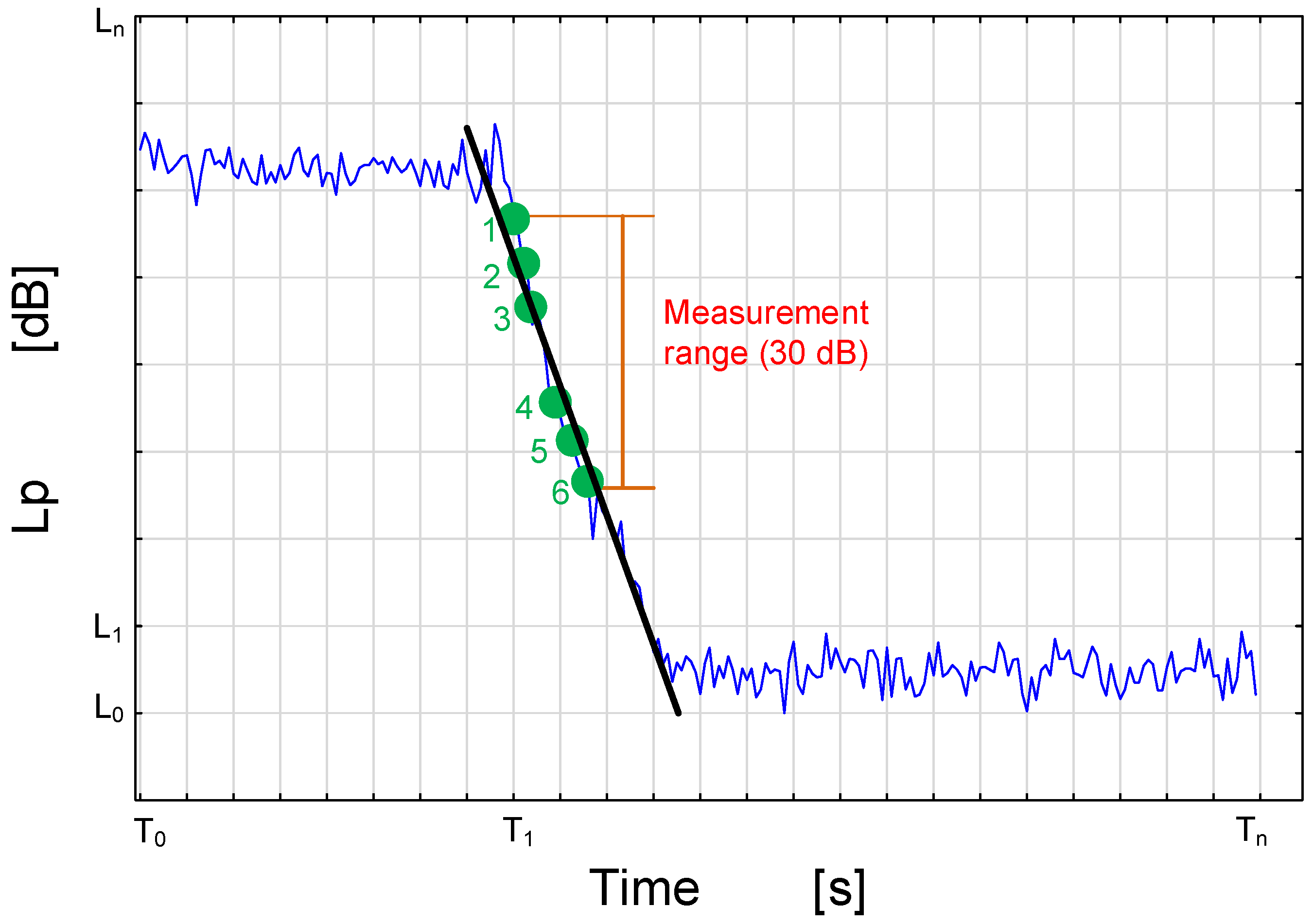
Figure 7.
Decay curves of 24 laboratory measurements. Each line represents a new measurement repetition.
Figure 7.
Decay curves of 24 laboratory measurements. Each line represents a new measurement repetition.

Figure 8.
Regression function from 24 fragments of sound decay curves for the frequency of 500 Hz.
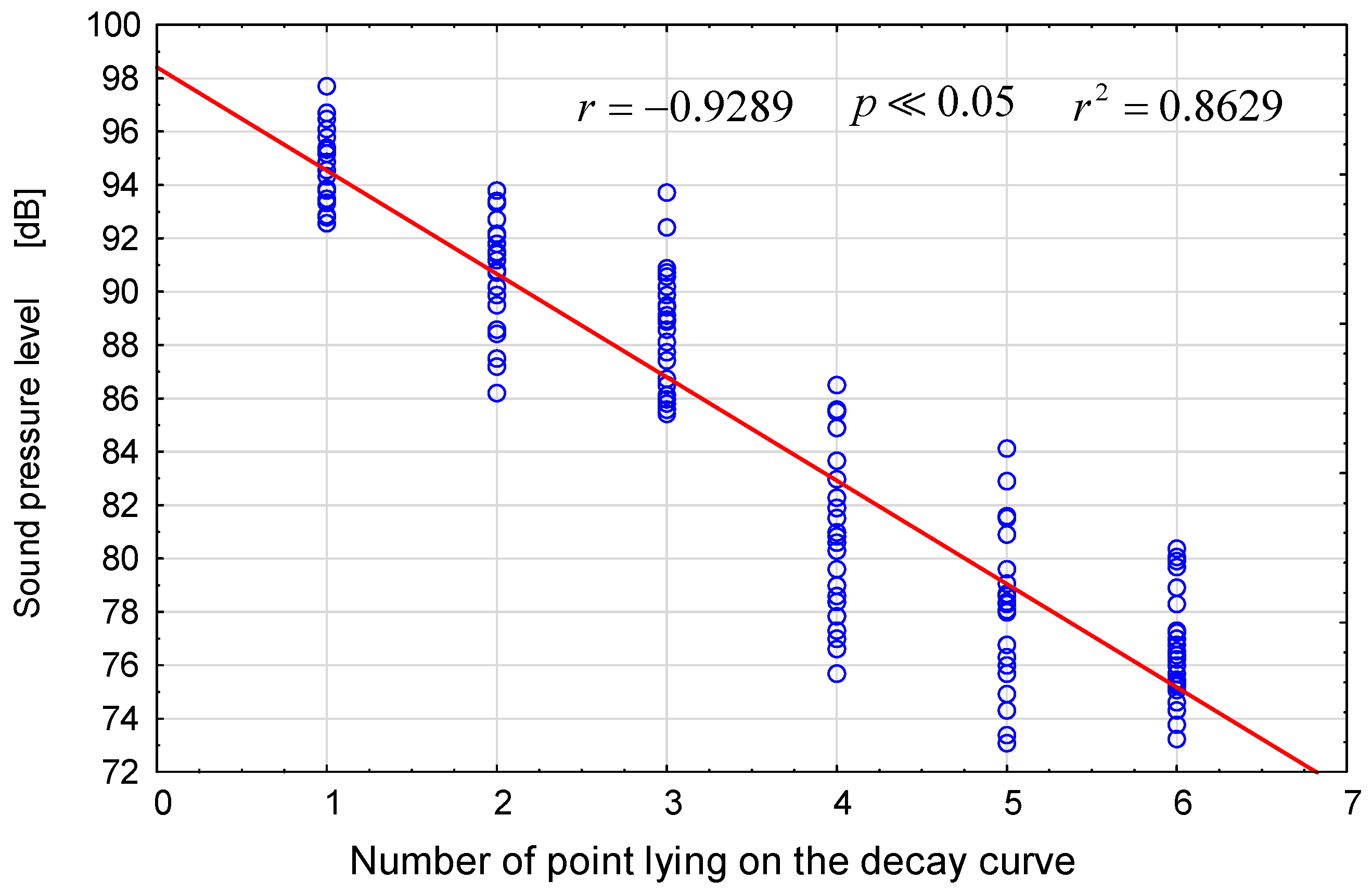
Figure 9.
Regression function from 24 fragments of decay curves for the frequency of 1000 Hz.

Figure 10.
Regression function from 24 fragments of decay curves for the frequency of 2000 Hz.

Figure 11.
Results of 72 reverberation time measurements—500 Hz.

Figure 12.
Decay curves from 72 measurements for the frequency of 500 Hz. Each line represents a new measurement repetition.
Figure 12.
Decay curves from 72 measurements for the frequency of 500 Hz. Each line represents a new measurement repetition.

Figure 13.
Regression function from 72 fragments of decay curves for the frequency of 500 Hz.

Disclaimer/Publisher’s Note: The statements, opinions and data contained in all publications are solely those of the individual author(s) and contributor(s) and not of MDPI and/or the editor(s). MDPI and/or the editor(s) disclaim responsibility for any injury to people or property resulting from any ideas, methods, instructions or products referred to in the content. |
© 2023 by the author. Licensee MDPI, Basel, Switzerland. This article is an open access article distributed under the terms and conditions of the Creative Commons Attribution (CC BY) license (https://creativecommons.org/licenses/by/4.0/).
Share and Cite
MDPI and ACS Style
Nowoświat, A. Determination of the Reverberation Time Using the Measurement of Sound Decay Curves. Appl. Sci. 2023, 13, 8607. https://doi.org/10.3390/app13158607
AMA Style
Nowoświat A. Determination of the Reverberation Time Using the Measurement of Sound Decay Curves. Applied Sciences. 2023; 13(15):8607. https://doi.org/10.3390/app13158607
Chicago/Turabian StyleNowoświat, Artur. 2023. "Determination of the Reverberation Time Using the Measurement of Sound Decay Curves" Applied Sciences 13, no. 15: 8607. https://doi.org/10.3390/app13158607
Note that from the first issue of 2016, this journal uses article numbers instead of page numbers. See further details here.